HAL Id: hal-00296205
https://hal.archives-ouvertes.fr/hal-00296205
Submitted on 27 Apr 2007
HAL is a multi-disciplinary open access
archive for the deposit and dissemination of
sci-entific research documents, whether they are
pub-lished or not. The documents may come from
teaching and research institutions in France or
abroad, or from public or private research centers.
L’archive ouverte pluridisciplinaire HAL, est
destinée au dépôt et à la diffusion de documents
scientifiques de niveau recherche, publiés ou non,
émanant des établissements d’enseignement et de
recherche français ou étrangers, des laboratoires
publics ou privés.
K. F. Boersma, H. J. Eskes, J. P. Veefkind, E. J. Brinksma, R. J. van der A,
M. Sneep, G. H. J. van den Oord, P. F. Levelt, P. Stammes, J. F. Gleason, et
al.
To cite this version:
K. F. Boersma, H. J. Eskes, J. P. Veefkind, E. J. Brinksma, R. J. van der A, et al.. Near-real time
retrieval of tropospheric NO2 from OMI. Atmospheric Chemistry and Physics, European Geosciences
Union, 2007, 7 (8), pp.2103-2118. �hal-00296205�
www.atmos-chem-phys.net/7/2103/2007/ © Author(s) 2007. This work is licensed under a Creative Commons License.
Chemistry
and Physics
Near-real time retrieval of tropospheric NO
2
from OMI
K. F. Boersma1,*, H. J. Eskes1, J. P. Veefkind1, E. J. Brinksma1, R. J. van der A1, M. Sneep1, G. H. J. van den Oord1,
P. F. Levelt1, P. Stammes1, J. F. Gleason2, and E. J. Bucsela2
1KNMI, De Bilt, The Netherlands 2NASA GSFC, Greenbelt, MD, USA
*now at: Harvard University, Cambridge, USA
Received: 7 November 2006 – Published in Atmos. Chem. Phys. Discuss.: 29 November 2006 Revised: 21 February 2007 – Accepted: 5 April 2007 – Published: 27 April 2007
Abstract. We present a new algorithm for the near-real
time retrieval – within 3 h of the actual satellite measurement – of tropospheric NO2 columns from the Ozone
Monitor-ing Instrument (OMI). The retrieval is based on the com-bined retrieval-assimilation-modelling approach developed at KNMI for off-line tropospheric NO2from the GOME and
SCIAMACHY satellite instruments. We have adapted the off-line system such that the required a priori information – profile shapes and stratospheric background NO2 – is now
immediately available upon arrival (within 80 min of obser-vation) of the OMI NO2 slant columns and cloud data at
KNMI. Slant columns for NO2 are retrieved using
differ-ential optical absorption spectroscopy (DOAS) in the 405– 465 nm range. Cloud fraction and cloud pressure are pro-vided by a new cloud retrieval algorithm that uses the ab-sorption of the O2-O2 collision complex near 477 nm.
On-line availability of stratospheric slant columns and NO2
pro-files is achieved by running the TM4 chemistry transport model (CTM) forward in time based on forecast ECMWF meteo and assimilated NO2information from all previously
observed orbits. OMI NO2 slant columns, after correction
for spurious across-track variability, show a random error for individual pixels of approximately 0.7×10¹⁵molec cm−2. Cloud parameters from OMI’s O2-O2 algorithm have
simi-lar frequency distributions as retrieved from SCIAMACHY’s Fast Retrieval Scheme for Cloud Observables (FRESCO) for August 2006. On average, OMI cloud fractions are higher by 0.011, and OMI cloud pressures exceed FRESCO cloud pressures by 60 hPa. A sequence of OMI observations over Europe in October 2005 shows OMI’s capability to track changeable NOxair pollution from day to day in cloud-free
situations.
Correspondence to: K. F. Boersma
1 Introduction
The daily global coverage and the nadir pixel size of 24×13 km2 make OMI on the Earth Observing System (EOS) Aura satellite well suited to observe the sources of air pollution with an unprecedented spatial and temporal cover-age. Recently, satellite-based observations of tropospheric NO2 have been proven useful in estimating anthropogenic
emissions of nitrogen oxides (Leue et al., 2001; Martin et al., 2003, 2006; Beirle et al., 2003; Richter et al., 2005; van der A et al., 2006), in observing emissions by soils (Jaegl´e et al., 2004), and in putting constraints on NOxproduction by
light-ning (Beirle et al., 2004, 2006; Boersma et al., 2005). Tropo-spheric NO2columns derived from the Global Ozone
Moni-toring Instrument (GOME) have been compared with outputs from various-scale models (Velders et al., 2001; Lauer et al., 2002; Savage et al., 2004; Ma et al., 2006). The results of the regional-scale chemistry-transport model CHIMERE have been evaluated against GOME and SCIAMACHY-derived tropospheric NO2 columns (Konovalov et al., 2004; Blond
et al., 2007). These comparisons have clearly demonstrated the potential of satellite NO2data sets for model evaluation
and emission estimates.
On the other hand, sometimes large and systematic dif-ferences persist between retrievals by different groups (van Noije et al., 2006), calling into question the quality of space-based constraints on NOxsources. But validation efforts for
various retrievals show acceptable accuracy (Heland et al., 2002; Petritoli et al., 2004; Martin et al., 2004, 2006; Petritoli et al., 2005; Cede et al., 2006; Ord´o˜nez et al., 2006; Schaub et al., 2006) for GOME and SCIAMACHY NO2.
The unique characteristics of OMI – the small pixel size and daily global coverage – allow for an important contribu-tion to air quality monitoring and modelling. GOME has a resolution of 320×40 km2, too coarse to resolve the areas with high emissions that are relevant in regional air qual-ity modelling, e.g. medium-sized cities. SCIAMACHY’s
horizontal resolution is 60×30 km2 but it needs six days to achieve global coverage. Despite the fact that interest-ing regional-scale daily variability has been observed with SCIAMACHY (Blond et al., 2007), it is not well suited for a day-to-day monitoring of air quality. The daily coverage of OMI has been an important motivation to set up the near-real time NO2retrieval system described in this paper.
An additional motivation originates from the data set of tropospheric NO2 columns retrieved from the GOME
and SCIAMACHY instruments that now spans more than 10 years (1996–2007) and is publicly available through (http://www.temis.nl). NO2 data sets from GOME and
SCIAMACHY have been retrieved with one and the same retrieval-assimilation-modelling approach described in Boersma et al. (2004) and show excellent mutual consistency (van der A et al., 2006). The OMI NO2-retrievals described
here are expected to add considerable value to the GOME and SCIAMACHY dataset.
Health regulations concerning air quality require a routine monitoring, typically on an hourly basis, of surface concen-trations of several species including NO2. Clearly, this
re-quirement cannot be directly fulfilled by satellite instruments in general, nor by OMI in particular. Nevertheless we antici-pate that instruments like OMI will make essential contribu-tions to air quality monitoring and modelling:
– Daily maps of NO2 columns by OMI (http://www.
temis.nl) show extensive transport features that are changing from day to day, and that are politically in-teresting as they directly show air pollution being trans-ported across national borders. These changeable dis-tributions can be directly compared with model output, and they constitute strong tests for the description of horizontal and vertical transport processes, as well as NOxremoval processes.
– A direct relationship exists between columns of NO2
and surface emissions of NOx. OMI data can thus
be combined with regional-scale models through in-verse modeling or data assimilation to adjust or improve emission estimates in the model and to detect unknown sources.
– Incidental releases, such as from major fires, can be monitored and quantified, and subsequent plumes can be tracked from day to day.
– A routine assimilation of satellite data may improve air quality “nowcasting” and forecasting capabilities, and may thereby contribute to the monitoring of emission and health regulations.
All these applications are new and largely untested. De-spite this, there exists a considerable interest in the com-munity to establish atmospheric chemistry data assimilation systems that will exploit the available satellite data sets of at-mospheric composition and air pollution. One example is the
European GEMS project (Global and regional Earth-system (Atmosphere) Monitoring using Satellite and in-situ data; (http://www.ecmwf.int/research/EU/projects/GEMS/) which is scheduled to deliver an operational atmospheric composi-tion assimilacomposi-tion system by 2009.
This paper presents a new retrieval algorithm designed for near-real time retrieval of tropospheric NO2 from OMI.
This algorithm differs from the standard, off-line OMI NO2 retrieval-procedure that is a joint NASA/KNMI effort
(Bucsela et al., 2006). These differences are discussed in Sect. 3.1. In Sect. 2 we discuss OMI characteristics and the fast data transport from the satellite to the retrieval com-puter system. The retrieval is discussed in Sect. 3, with a focus on the innovations with respect to previous NO2
col-umn retrieval work at KNMI. Section 4 is devoted to errors in the NO2slant columns. The stratospheric correction and
computation of the air mass factor (AMF) are described in Sect. 5. As SCIAMACHY and OMI cloud retrieval use dif-ferent spectral features, we also discuss in Sect. 5 the con-sistency of the OMI O2−O2 cloud product with the
SCIA-MACHY FRESCO cloud retrievals. In Sect. 6 we show some examples of OMI’s capabilities, followed by conclusions in Sect. 7.
2 OMI overview
2.1 Ozone Monitoring Instrument
The Dutch-Finnish Ozone Monitoring Instrument (OMI) on NASA’s EOS Aura satellite is a nadir-viewing imaging spec-trograph measuring direct and atmosphere-backscattered sunlight in the ultraviolet-visible (UV-VIS) range from 270 nm to 500 nm (Levelt et al., 2006a). EOS Aura was launched on 15 July 2004 and traces a Sun-synchronous, polar orbit at approximately 705 km altitude with a period of 100 min and a local equator crossing time between 13:40 and 13:50 local time. In contrast to its predecessors GOME and SCIAMACHY, instruments operating with scanning mir-rors and one-dimensional photo diode array detectors, OMI has been equipped with two two-dimensional CCD detec-tors. The CCDs record the complete 270–500 nm spectrum in one direction, and observe the Earth’s atmosphere with a 114◦ field of view, distributed over 60 discrete viewing an-gles, perpendicular to the flight direction. OMI’s wide field of view corresponds to a 2600 km wide spatial swath on the Earth’s surface for one orbit, large enough to achieve com-plete global coverage in one day. The exposure time of the CCD-camera measures 2 s, corresponding to a spatial sam-pling of 13 km along track (2 s×6.5 km/s, the latter being the orbital velocity projected onto the Earth’s surface). Across track the size of an OMI pixel varies with viewing zenith an-gle from 24 km in the nadir to approximately 128 km for the extreme viewing angles of 57◦at the edges of the swath.
OMI has three spectral channels; UV1 (270–310 nm) and UV2 (310–365 nm) are covered by CCD1. CCD2 covers the VIS-channel from 365-500 nm with a spectral sampling of 0.21 nm and a spectral resolution of 0.63 nm. It is in this channel that the spectral features of NO2are most prominent.
The spectral sampling rate (resolution/sampling) is ∼ 3, large enough to avoid spectral undersampling or aliasing difficul-ties in the spectral fitting process. A polarization scrambler makes the instrument insensitive to the polarization state of the reflected Earth radiance to less than 0.5%.
During nominal operations OMI takes one measurement of the solar irradiance per day. Radiometric calibration is accomplished in-flight by a series of special on-board mea-surements that involve monitoring detector degradation with a white-light source, and dark signal measurements when OMI is at the dark side of the Earth. Spectral calibration is achieved by a cross-correlation of Fraunhofer lines in theo-retical and observed in-flight irradiance spectra. For more de-tails on the instrument and calibration procedures, the reader is referred to Dobber et al. (2005, 2006).
Retrievals of ozone column and vertical distribution (as well as BrO and OClO columns) are meant to address the first EOS Aura science question whether the ozone layer is recovering. Of no less importance are the retrievals of trace gases related to air pollution and the production of photo-chemical smog, i.e. NO2, HCHO (Kurosu et al., 2005), and
SO2(Krotkov et al., 2006). In addition, cloud and aerosol
parameters, and UV-B surface flux are derived from OMI. For an overview of EOS-AURA and OMI targets, see Levelt et al. (2006b).
2.2 Data transport
Unprocessed OMI science data are down-linked once per or-bit (100 min) to one of the Ground Stations (Alaska, Svals-bard (Spitsbergen), or Wallops (Virginia)). Subsequently the OMI data are sent to the EOS Data Operations System (EDOS) at NASA GSFC in Maryland (USA). At GSFC, pro-cessing of raw OMI data results in Rate-Buffered Data, Ex-pedited Data, and Production Data. Near-real time process-ing is based on Rate-Buffered Data (RBD). RBD data are made available with the highest priority, at the expense of data integrity. The other data types are scheduled for off-line level 2 retrievals.
EDOS forwards the RBD data to the OMI Science Investigator-led Processing System (SIPS), where produc-tion starts as soon as all engineering, ancillary and science data have been received. Then, the resulting level 0 data sets (in Analog to Digital Units) are processed into level 1b data, i.e. estimated radiances and irradiances in units of W/m2/nm(/sr) (van den Oord et al., 2006). The only differ-ence with standard production at this time is that the near-real time processing uses the predicted altitude and ephemeris data received from the spacecraft rather than definitive al-titude and ephemeris data. Using predicted orbital
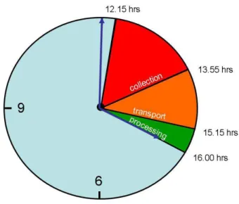
parame-Fig. 1. OMI science data is linked down to ground stations once per
orbit, resulting in a time delay between the OMI observations and reception at the ground station of at most 100 min. The collection, time-ordering, consecutive transfers, and level 1b and 2 process-ing, takes approximately 80 min. Final processprocess-ing, image genera-tion and web publishing generally occurs within 45 min.
ters may lead to errors in geolocation parameters (latitude, longitude, solar, viewing, and azimuth angles), but in prac-tice these errors are small. Once OMI level 1b data has been generated at the SIPS, the O2−O2cloud level 1–2
al-gorithm (Acarreta et al., 2004) is run, followed by the DOAS ozone (Veefkind and De Haan, 2002) and NO2slant column
spectral fitting retrieval algorithms. As soon as the ozone and NO2 slant column files are available, they are picked
up by the OMI Dutch Processing system (ODPS) and for-warded to the processing system at KNMI developed within the DOMINO project (see acknowledgment). Subsequent steps are intrinsic parts of the near-real time retrieval algo-rithm and are described in the next section.
Typical data volumes per orbit are 450 MB level 0 data, 400 MB level 1b data, and 17 MB NO2 slant column data
(including cloud retrievals). Processed orbital data arrives at KNMI on average within three hours after the start of an orbit. An orbit takes 100 min (indicated as the red part of Fig. 1) and the process described above (downlink, transfer to EDOS, transfer to SIPS, level 1b and 2 processing, and trans-fer to KNMI) takes 80 min (the orange part in Fig. 1). Final processing from NO2slant columns to tropospheric vertical
columns is typically faster than 2 min on a linux worksta-tion. Including the generation of images and web publishing, the processing step takes less than 45 min (the green part of Fig. 1), so that data and images are available for the public at approximately 16:00 local time.
3 Algorithm description
3.1 Heritage: the retrieval-assimilation-modelling ap-proach
The near-real time NO2 retrieval algorithm (DOMINO
ver-sion: TM4NO2A-OMI v0.8, February 2006) is based on the retrieval-assimilation-modelling approach (hereafter: RAM) described in Boersma et al. (2004). The RAM-approach has been applied at KNMI to generate a tropospheric NO2data
base from GOME and SCIAMACHY measurements. The RAM approach consists of a three-step procedure:
1. a slant column density is determined from a spectral fit to the Earth reflectance spectrum with the so-called DOAS approach (differential absorption spectroscopy, e.g. Platt, 1994; Boersma et al., 2002; Bucsela et al., 2006),
2. the stratospheric contribution to the slant column is es-timated from assimilating slant columns into a CTM in-cluding stratospheric chemistry and wind fields, and 3. the residual tropospheric slant column is converted into
a vertical column by application of a tropospheric air mass factor (AMF).
The standard, off-line NO2product (Bucsela et al., 2006) and
the near-real time retrieval have step 1 in common. This step is discussed in detail in Sect. 3.2 and 3.3. Step 2 and 3 are (partly) different between the OMI off-line and NRT algo-rithms. Table 1 summarizes similarities and differences be-tween the two retrievals.
A NO2 data set (from April 1996 onwards) has been
generated with the RAM-approach from GOME and SCIA-MACHY. The set contains tropospheric NO2columns along
with error estimates and averaging kernels (Eskes and Boersma, 2003) for every individual pixel and is publicly available through http://www.temis.nl. Schaub et al. (2006) showed that RAM-GOME tropospheric NO2over Northern
Switzerland in the period 1996–2003 compares favourably to NO2profiles observed with in-situ techniques. Blond et al.
(2007) reported considerable consistency between RAM-SCIAMACHY tropospheric NO2columns and both surface
observations as well as simulations from the regional air-quality model CHIMERE over Europe, especially over mod-erately polluted rural areas. Merged GOME and SCIA-MACHY observations showed a distinct increase in NO2
columns from 1996 to 2003 over China, consistent with a strong growth of NOx emissions in that area (van der A
et al., 2006). Moreover, this paper showed an almost seam-less continuity from GOME to SCIAMACHY NO2 values
retrieved with the same RAM-approach. This finding pro-vides confidence in the consistency of the two data sets and their retrieval method, even though they originated from two different instruments (with similar overpass times of 10:30 (GOME) and 10:00 local time (SCIAMACHY)).
Tropospheric NO2columns are retrieved as follows:
Vt r=
S − Sst
Mt r(xa,tr,b)
, (1)
with S the slant column density from step 1, Sst the
strato-spheric slant column obtained from step 2, and Mt r the
tro-pospheric AMF that depends on the a priori NO2profile xa,tr
and the set of forward model paramaters b including cloud fraction, cloud pressure, surface albedo, and viewing geome-try. The vertical sensitivity of OMI NO2 strongly depends
on surface albedo and the presence of clouds (Eskes and Boersma, 2003).
For the RAM-approach and the NRT-retrieval, AMFs and averaging kernels are computed with a pseudo-spherical ver-sion of the DAK radiative transfer model (Stammes, 2001) as described in Boersma et al. (2004). Given the best estimate of the forward model parameters the DAK forward model simulates the scattering and absorbing processes that define the average optical path of photons from the Sun through the atmosphere to the OMI.
Also similar as in our RAM-approach for off-line re-trievals, we obtain here the a priori NO2profile shapes (xa,tr)
from the global chemistry-transport model TM4 at a resolu-tion of 2◦latitude by 3◦longitude and 35 vertical levels ex-tending up to 0.38 hPa. Given the few available in situ NO2
measurements, a global 3-D model of tropospheric chemistry is the best source of information for the vertical distribution of NO2 at the time and location of the OMI measurement.
The TM4 model is driven by forecast and analysed six hourly meteorological fields from the European Centre for Medium Range Weather Forecast (ECMWF) operational data. These fields include global distributions for horizontal wind, sur-face pressure, temperature, humidity, liquid and ice water content, cloud cover and precipitation. A mass conserving preprocessing of the meteorological input is applied accord-ing to Bregman et al. (2003). Key processes included are mass conserved tracer advection, convective tracer transport, boundary layer diffusion, photolysis, dry and wet deposition as well as tropospheric chemistry including non-methane hy-drocarbons to account for chemical loss by reaction with OH (Houweling et al., 1998). In TM4, anthropogenic and natural emissions of NOx are based on results from the EU
POET-project (Precursors of Ozone and their Effects on the Tro-posphere) for the year 1997 (Olivier et al., 2003). Including free tropospheric emissions from air traffic (0.8 Tg N/yr) and lightning (5 Tg N/yr), total NOxemissions for 1997 amount
to 46 Tg N/yr.
Because OMI does not detect the O2A band at 760 nm,
we use cloud parameters retrieved from the VIS-channel us-ing the O2−O2absorption feature at 477 nm (Acarreta et al.,
2004). The cloud retrieval is based on the same set of as-sumptions (i.e. clouds are modelled as Lambertian reflec-tors with albedo 0.8) as the FRESCO-algorithm (Koelemei-jer et al., 2001). Before launch, the precision of the O2−O2
Table 1. Overview of the two OMI tropospheric NO2retrievals.
OMI standard product (Bucsela et al., 2006) OMI near-real time (this work)
Slant column DOAS (405–465 nm) DOAS (405–465 nm)
Across-track variability correction Correction factors Correction factors based on 24-h data1 computed per-orbit2 Stratospheric slant column Wave-2 fitting along zonal band Data assimilation in TM4 AMF - cloud parameters O2−O2(Acarreta et al., 2004) O2−O2(Acarreta et al., 2004) AMF - surface albedo GOME(Koelemeijer et al., 2003) TOMS/GOME3
AMF - profile shape Yearly average profile shapes from Collocated daily output at GEOS-Chem (2.5◦×2◦)4 overpass time from TM4 (3◦×2◦) AMF - ghost column Not included Implicit in AMF definition
1In the standard product, mean slant columns are adjusted for a given cross-track position to the mean value at all positions. The mean slant column and the mean initial AMF for each cross-track position are computed from 24-h of data using measurements obtained at latitudes between ±55◦. These are used to generate a set of 60 correction constants, one for each cross-track position, which are subtracted from the slant column values before computation of the vertical columns.
2The correction for the near-real time retrieval is described in Sect. 4.1.
3Surface albedo fields are taken from a combination of Herman and Celarier (1997) and Koelemeijer et al. (2003) as described in Boersma et al. (2004).
4AMFs are corrected based on average a priori profile shapes when the retrieved slant column is larger than the estimated stratospheric slant column (Bucsela et al., 2006).
et al. (2004) with encouraging results. In Sect. 5.2.1 we test the accuracy of the O2−O2 cloud parameters by
compar-ing them to FRESCO cloud parameters retrieved by SCIA-MACHY on the same days and same locations.
As for GOME and SCIAMACHY retrievals, we use a surface albedo database derived from TOMS and GOME Lambert-equivalent reflectivity (LER) measurements at 380 nm and 440 nm as described in Boersma et al. (2004). These monthly average surface albedo maps have a spa-tial resolution of 1◦×1.25◦ and represent climatological (monthly) mean situations. The uncertainty in the surface albedo is estimated to be approximately 0.01 (Koelemeijer et al., 2003; Boersma et al., 2004).
In summary, the near-real time algorithm is based on the RAM-approach used for GOME and SCIAMACHY re-trievals at KNMI. The main differences with RAM are: (1) near-real time requirement, (2) different spectral fitting method, and (3) cloud inputs derived from (similar but) dif-ferent algorithms.
3.2 Near-real time retrieval
In the RAM-approach, the estimated stratospheric NO2
col-umn (step 2) and the modelled profile shape (required for step 3), are provided by off-line assimilation and modelling based on analysed ECMWF meteorological data. In contrast, for the NRT-retrieval, the assimilation and modelling steps are operational, based on daily ECMWF meteorological analy-ses and forecasts.
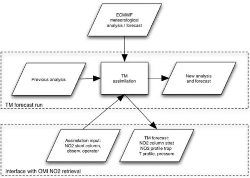
The NRT-retrieval consists of two distinct subsystems.
The first is the TM forecast subsystem shown in Fig. 2. This forecast system is run once per day, as soon as meteoro-logical data becomes available. The second subsystem is activated each and every time that new OMI data becomes available, and incorporates the model information provided by subsystem 1.
In the forecast subsystem (1), the actual chemical state of the atmosphere is based on the analysis and forecast run starting from the analysis of the previous day. The update consists of running the chemistry-transport model forward in time with the forecast ECMWF meteorological data and the assimilation of all available OMI NO2 slant columns
mea-surements. The updated analysis, the new actual state, is then stored as input for a subsequent time step. The outputs are the necessary inputs to the near-real time subsystem (2); the stratospheric NO2column and the NO2and temperature
pro-files (needed in AMF computations).
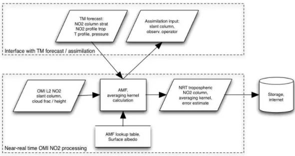
The NRT-subsystem is illustrated in Fig. 3. As soon as an orbit of observed NO2slant columns arrives at KNMI, the
forecast TM stratospheric slant column, is ready and is sub-tracted. Subsequently, the residual tropospheric slant column is converted into a vertical column by the tropospheric AMF. The AMF is computed as described as in 3.1. The averaging kernel is also calculated for output and furthermore serves as the observation operator required in the assimilation part of the TM forecast subsystem.
Fig. 2. Flowchart for the DOMINO forecast/assimilation subsystem. The lowest part shows the input-output interface with the
NRT-subsystem.
3.3 Slant column retrieval
A second difference between the OMI near-real time and RAM off-line implementations is the wide spectral win-dow that is used in the DOAS retrieval. For GOME and SCIAMACHY, it has been conventional wisdom that a 425– 450 nm window yields the most precise and stable fitting results. For OMI a much wider fit window, 405–465 nm, has been proposed by Boersma et al. (2002) in order to compensate for OMI’s lower signal-to-noise ratio (approx-imately 1400 under normal mid-latitude conditions) com-pared to GOME and SCIAMACHY (approximately 2000, Bovensmann et al., 1999) in this wavelength region. Pre-flight testing showed that a least squares fitting of reference spectra from NO2, O3, a theoretical Ring function, and a 3rd
order polynomial to the reflectance spectrum yields results that are stable for multiple viewing geometries with a bet-ter than 10% NO2 slant column precision (Boersma et al.,
2002). Including H2O and O2−O2did not affect the fitted
slant columns. The NO2absorption cross section spectrum
is taken from Vandaele et al. (1998), who tabulated the cross section at different temperatures. To account for the temper-ature sensitivity of the NO2 cross section spectrum an
ef-fective atmospheric temperature is calculated for the NO2
along the average photon path. Subsequently an a posteri-ori correction for the difference between the computed effec-tive temperature and the 220 K cross section spectrum used in the fitting procedure is applied (Boersma et al., 2002). The ozone absorption cross section spectrum is taken from WMO
(1975) and the theoretical Ring spectrum from De Haan (private communication, 2006) based on irradiance data by Voors et al. (2006). All reference spectra have been con-volved with the OMI instrument transfer function (Dobber et al., 2005). OMI NO2slant column retrieval with synthetic
and flight model data (Dobber et al., 2005) yields results that fulfill the OMI science requirement of better than 10% slant column precision (Boersma et al., 2002; Bucsela et al., 2006). However, upon first inspection of actual flight-data, system-atic enhancements in the OMI NO2slant columns show up at
specific satellite viewing angles. This has also been reported by Kurosu et al. (2005) for HCHO-retrievals.
4 Slant column density errors
4.1 Across-track variability
Calibration errors in the level 1b OMI irradiance measure-ments used here are likely responsible for across-track vari-ability observed in the NO2 slant columns. This variability
will likely be significantly reduced in future level 1b releases with improved calibration data (expected in Spring 2007), using daily dark current corrections. Across-track variabil-ity appears as constant offsets for specific satellite viewing angles along an orbit, allowing for an a posteriori correction: 1. Determine the orbital segment (50 along track by 60 across track pixels in size) with the minimum variance in NO2columns.
Fig. 3. Flowchart for the DOMINO NRT-subsystem. The upper part shows the input-output interface with the
forecast/assimilation-subsystem (the lower part of Fig. 2).
2. Within this window, average the 50 NO2columns with
the same viewing angle. This gives 60 average across-track NO2columns.
3. Separate low and high frequencies of the across-track columns with a Fourier analysis.
4. Perform the correction by subtracting the (high-frequency) across-track variability for all across-track rows along the orbit.
In this scheme, the selection of the minimum variance win-dow avoids areas with large anthropogenic emissions. The high-frequencies are then interpreted as the across-track vari-ability due to calibration errors in the OMI level 1b data. Similarly, the low frequencies describe any (weak, strato-spheric) natural variability. The low frequencies are de-scribed by the first three Fourier terms. Subsequently we subtract the high-frequency signal obtained for the minimum variance window for all rows along the orbit. If it turns out to be not possible to determine a correction for a particular or-bit, the across-track variability correction from the previous orbit is taken. Figure 4 shows corrections for across-track variability computed from 10 consecutive orbits measured on the same day (22 September 2004). Although the corrections have been computed from independent data, they are similar. This justifies taking the correction determined from the pre-vious orbit if it cannot be determined from the actual orbit. Furthermore, Fig. 4 provides evidence that irradiance data are most likely at the basis of the across-track variability. All orbits shown have been retrieved with the same irradiance measurement. However, when the correction was plotted for
0 20 40 60 Across track -4 -2 0 2 4 NO 2 correction (x 10 15 molec. cm -2)
Fig. 4. Across-track variability corrections, computed with the method described in Sect. 4.1, for 10 consecutive orbits on 22 September 2004. Every orbital correction is shown with a unique colour.
the first orbit retrieved with a new irradiance measurement, a distinctly different correction pattern was seen (not shown). 4.2 Slant column precision
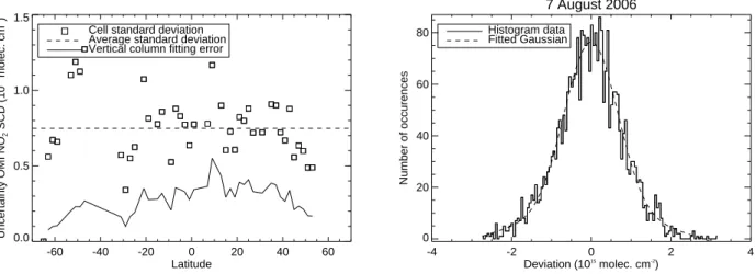
We present here a statistical analysis of OMI NO2columns
observed over separate 2◦×2◦boxes in the meridional band between 178◦and 180◦W. The basic assumption is that the OMI pixels within a 2◦×2◦box observe the same total ver-tical column over this clean part of the Pacific Ocean. Any variability in the observed total vertical columns is assumed
-60 -40 -20 0 20 40 60 Latitude 0.0 0.5 1.0 1.5 Uncertainty OMI NO 2 SCD (10 15 molec. cm -2)
Cell standard deviation Average standard deviation Vertical column fitting error
7 August 2006 -4 -2 0 2 4 Deviation (1015 molec. cm-2 ) 0 20 40 60 80 Number of occurences Histogram data Fitted Gaussian
Fig. 5. Left panel: standard deviation of slant columns within a 2◦×2◦(longitudes between 178◦and 180◦W) box as a function of latitude. The dashed line shows the meridional average of the standard deviations for all the boxes. The solid line shows the contribution of the (slant column) fitting error to the vertical column error M (i.e. σS/M). Right panel: distribution of member deviations from box means for 2893 pixels. The dashed line shows a Gaussian function fitted to the histogram data. The width of the Gaussian corresponds to a slant column error of 0.67×10¹⁵molec cm−2.
to originate from errors in the slant columns if the ensem-ble of AMFs within a box has little variability. Boxes with appreciable AMF variability have been rejected if the box-mean vertical column computed by averaging the ensemble of individual slant columns ratioed by a box-mean AMF (V′)
differed by more than 0.1% from the box-mean vertical col-umn computed by averaging the ensemble of individual slant columns ratioed by the original AMFs (V ). We find that for most of the 2◦×2◦boxes between 60◦N and 60◦S, V and V′
do not differ by more than 0.1%, and thus the slant columns have been observed under almost identical viewing geome-tries. For these boxes, we take the standard deviation of the ensemble of slant-column as the estimate for the precision of the slant columns.
For 7 August 2006, we computed estimates for the slant column errors for every box between 60◦S and 60◦N. The results are shown in Fig. 5 (left panel) for boxes with a rel-ative difference between V and V′ of less than 0.1%. The
figure shows that there is no appreciable change of fitting error with latitude. Averaged over all latitudes, the fitting error is close to 0.75×10¹⁵molec cm−2 (dashed line). For the vertical column error, the contribution from the fitting error is smaller than 0.4×10¹⁵molec cm−2(solid line,
com-puted as σS/M). Figure 5 (right panel) shows the
distribu-tion of all member deviadistribu-tions from box means in a histogram (n=2893). The distribution closely follows a Gaussian shape that is fitted to the histogram data. The fact that the distribu-tion follows a Gaussian distribudistribu-tion is consistent with our assumption that the variability within each box is dominated by random errors in the slant columns, originating from mea-surement noise and possible residuals of the correction pro-cedure. The corresponding width of the Gaussian for this
day is 0.67×10¹⁵molec cm−2, and we interpret this as our estimate for the average slant column error of all 2893 pixels we investigated on 7 August 2006. The slant column error is the combined error from fitting noise and from any resid-ual across-track variability. We also looked into a few other days and other longitude bands with different across-track variability corrections, and found very similar numbers.
The slant column error for an individual OMI pixel is somewhat larger than the better-than-10% (≈0.3×10¹⁵ molec cm−2) number quoted in Boersma et al. (2002). This number was computed from synthetic spectra (i.e. without across-track variability) under the assumption that 4 OMI pixels would be binned (increasing signal-to-noise by a fac-tor of 2). For individual pixels, the OMI fitting error is larger than the 0.45×10¹⁵molec cm−2found for GOME (Boersma
et al., 2004) and SCIAMACHY (I. DeSmedt, private commu-nication), consistent with the higher signal-to-noise ratios for individual GOME and SCIAMACHY pixels than for OMI pixels.
5 Stratospheric contribution and tropospheric air mass
factor
5.1 Stratospheric slant column
The stratospheric component of the NO2slant column is
es-timated by data-assimilation of OMI slant columns in TM4:
– Modelled NO2profiles are convolved with the
appropri-ate averaging kernel to give model-predicted slant col-umn densities. We take model fields that are closest in time to the mean OMI orbit time (model information is stored in UT with 30 min increments, 48 fields per day).
This limits differences between observation and model times in the assimilation to at most 55 min (±25 from actual vs. mean orbit time, ±30 from model vs. mean orbit time). Taking model fields closest in time is rele-vant only at high latitudes where local time differences across an OMI swath are considerable and could lead to large assimilation errors if the model was just sam-pled at 13:30 local time. Rejecting retrievals with so-lar zenith angles >80◦, we avoid regions with day-night transitions. The differences between observed and mod-elled columns (the model innovations) are used to force the modelled columns to generate an analysed state that is based on the modelled NO2distribution and the OMI
observations.
– The forcing depends on weights (from observation rep-resentativeness and model errors) attributed to model and observation columns. The observation error is set to A times the modelled tropospheric slant column plus B times the modelled (assimilated) stratospheric slant column. A and B are relative errors, and are chosen as A=4 and B=0.25. This implies that the observation error rapidly increases for modelled tropospheric ver-tical columns larger than or of the order of 0.5×10¹⁵ molec cm−2. As a consequence, moderately and highly polluted regions obtain a small weight in the assimi-lation. The ratio A/B roughly reflects the high uncer-tainties in the tropospheric retrieval as compared to the stratosphere.
– The forcing equation (based on the Kalman filter technique) is solved with the statistical interpolation method. This involves a covariance matrix that de-scribes the forecast error and spatial correlations. The most important characteristics of this forecast covari-ance matrix are: (1) the conservation of modelled pro-file shapes. The altitude dependence of the forecast error is set to be proportional to the local NO2profile
shape. (2) The horizontal correlation model function is assumed to follow a Gaussian shape with an 1/e corre-lation length of 600 km. This length was derived from the assimilation of ozone in the stratosphere (Eskes et al., 2003) and should be a reasonable guess for strato-spheric NO2as well. (3) In addition we introduce a
cor-relation scaling to reduce the corcor-relation with increas-ing differences in concentration (Riishøjgaard, 1998). This avoids problems with negative concentrations near sharp gradients that occur for instance at the polar vor-tex edge. (4) The vertical distribution of the assimilation increments is determined by the covariance matrix and the averaging kernel profile. The kernel peaks in most cases in the stratosphere, which is an additional reason why the adjustment caused by the assimilation is mainly taking place in the stratosphere.
– The adjustments made by the assimilation are therefore mainly occurring in the stratosphere at places where the tropospheric concentrations are low. The stratospheric information inserted by the assimilation is transported to the stratosphere above more polluted areas by the ad-vection in the model.
– The model NOxspecies (NO, NO2, NO3, N2O5, HNO4)
are assumed to be fully correlated and are all scaled in the same way as NO2.
– Based on the most recent analysed state, a forecast run of the model predicts the stratospheric field. This is used by the near-real time retrieval branch as shown in Fig. 2. For further reading on the assimilation method we refer to Eskes et al. (2003). The advantage of the approach is that slant column variations due to stratospheric dynamics are now accounted for in the retrieval. The purpose is to im-prove the detection limit for tropospheric NO2columns. An
additional advantage is that the assimilation scheme provides a statistical estimate of the uncertainty in the stratospheric slant column. Generally, this uncertainty is on the order of 0.1–0.2×10¹⁵ molec cm−2, much smaller than the slant col-umn uncertainty. Hence, the detection limit in our method is mainly determined by the random slant column error (σS)
that is easily averaged out by taking large numbers of obser-vations. Not accounting for stratospheric dynamics however, would lead to systematic errors in the estimate of the strato-spheric column (Boersma et al., 2004) that cannot easily be averaged out and would raise the detection treshold. 5.2 Tropospheric air mass factor
We convert the tropospheric slant column into a vertical col-umn by using a tropospheric AMF (Eq. 1). For OMI NRT we follow as much as possible the same approach (same look-up tables, computational methods) as for the GOME and SCIA-MACHY data set described in Sect. 3.1. But the forward model input parameters cloud fraction and cloud pressure differ between the OMI NRT and the GOME and SCIA-MACHY RAM retrievals. This, along with the much finer spatial resolution of OMI compared to GOME, is expected to lead to different error budgets for OMI tropospheric NO2
than for GOME and SCIAMACHY. 5.2.1 Cloud parameters
DOAS-type retrievals are very sensitive to errors in cloud parameters. Boersma et al. (2004) showed that errors in FRESCO cloud fractions of ±0.05 lead to retrieval errors of up to 30% for situations with strong NO2 pollution. Errors
in the cloud pressure may also affect retrievals, especially in situations where the retrieved cloud top is located within a polluted layer. In such situations, errors in the cloud pressure of 50 hPa lead to retrieval errors of up to 25%.
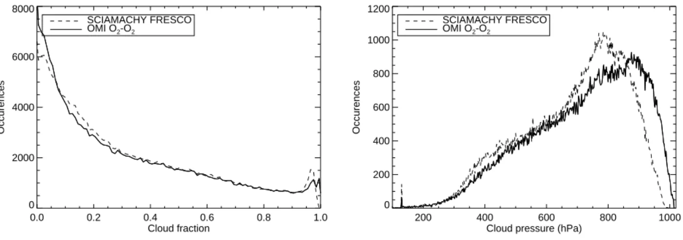
0.0 0.2 0.4 0.6 0.8 1.0 Cloud fraction 0 2000 4000 6000 8000 Occurences SCIAMACHY FRESCO OMI O2-O2 200 400 600 800 1000 Cloud pressure (hPa)
0 200 400 600 800 1000 1200 Occurences SCIAMACHY FRESCO OMI O2-O2
Fig. 6. Left panel: histogram of 0.5×0.5× gridded effective cloud fractions from SCIAMACHY FRESCO (dashed line) and OMI O2−O2 for seven consecutive days (5–11 August 2006). Right panel: histogram of 0.5×0.5× gridded effective cloud pressures from SCIAMACHY FRESCO (dashed line) and OMI O2−O2for seven consecutive days (5–11 August 2006). Only observations with a cloud fraction higher or equal to 0.05 are shown.
Here we evaluate any differences between cloud parame-ters retrieved by SCIAMACHY and OMI. FRESCO applied on GOME measurements compared favourably to AVHRR (Koelemeijer et al., 2001) and ISCCP (Koelemeijer et al., 2002) cloud fractions (differences <0.02) and cloud pressure (differences <50-80 hPa). More relevantly, Fournier et al. (2006) showed that FRESCO cloud parameters are in good agreement with other SCIAMACHY cloud algorithms, and estimate that the accuracy of the effective cloud fraction from FRESCO is better than 0.05 for all surfaces except snow and ice.
The retrieval methods for SCIAMACHY (FRESCO) and OMI (O2−O2) are based on the same principles, i.e. they
both retrieve an effective cloud fraction, that holds for a cloud albedo of 0.8, and to do so, they both use the continuum top-of-atmosphere reflectance as a measure for the brightness, or cloudiness, of a scene. Furthermore they both use the depth of an oxygen band as a measure for the length of the average photon path from the Sun, through the atmosphere back to the satellite instrument. The length of this light path is con-verted to cloud pressure. On the other hand, there are signifi-cant differences between the cloud parameter retrievals from SCIAMACHY and OMI:
1. FRESCO uses reflectances measured inside and outside of the strong oxygen A band (758–766 nm), whereas OMI uses the weakly absorbing O2−O2band at 477 nm.
2. FRESCO and O2−O2 have different sensitivities to
cloud pressure. This originates from the use of absorp-tion by a single molecule (FRESCO, O2A band), scaled
with oxygen number density, versus the use of absorp-tion by a collision complex (O2−O2), scaled with
oxy-gen number density squared. Although this dependence
is taken into account in the retrieval algorithm, it is ex-pected to lead to higher cloud pressures for the O2−O2
cloud algorithm.
3. FRESCO does not account for Rayleigh scattering, whereas the O2−O2 algorithm does. Not accounting
for Rayleigh scattering leads to cloud pressures to be underestimated for small cloud fractions (Wang et al., 2006).
4. SCIAMACHY observes clouds at 10:00, and OMI at 13:45 local time.
Because SCIAMACHY and OMI observe the Earth at dif-ferent times, FRESCO and O2−O2 cloud parameters
can-not be compared directly. However, since temporal vari-ation in global cloud fraction and cloud pressure between 10:00 and 13:45 local time is small (Bergman and Salby, 1996), frequency distributions of cloud parameters may be compared as an evaluation of consistency between the two. Here we compare SCIAMACHY FRESCO cloud retrievals version SC-v4 (August 2006, with improved desert surface albedos) to OMI O2−O2retrievals v1.0.1.1 (available since
7 October 2005, orbit 6541). We focus on locations between 60◦N and 60◦S to avoid situations with ice and snow, where
cloud retrieval traditionally is difficult. We gridded FRESCO and O2−O2cloud parameters to a common 0.5◦×0.5◦grid
and selected only grid cells filled with successfully retrieved cloud values for both FRESCO and O2−O2. Doing so, we
obtain SCIAMACHY and OMI cloud parameter distribu-tions on a spatial grid comparable to the SCIAMACHY grid (30×60 km2) that have been sampled on the same days and locations.
Figure 6 (left panel) shows the cloud fraction distribution as observed by FRESCO (dashed line) and O2−O2
aver-aged over the period 5–11 August 2006. The distributions show a high degree of similarity, with the smallest effective cloud fractions observed most often. The differences be-tween the two distributions are most appreciable for small effective cloud fractions, with OMI more frequently observ-ing cloud fractions smaller than 0.05, and SCIAMACHY more frequently observing cloud fractions in the 0.05-0.20 range. These differences are likely related to different sur-face albedo data bases used in the cloud retrievals, and the way effective cloud fractions outside the 0.0–1.0 range are treated. The O2−O2retrieval uses the TOMS/GOME surface
albedo datasets at 463 and 494.5 nm, consistent with albe-dos used for NO2 AMF computations. But for FRESCO,
the GOME albedo dataset at 760 nm is used. Since OMI’s horizontal resolution is much finer than the 1◦×1◦ surface
albedo datasets, this will lead to cloud fraction errors, espe-cially for small cloud fractions. On average for 5–11 August 2006, FRESCO observes a mean effective cloud fraction of 0.311, and O2−O2observes 0.300. The small mean
differ-ence between FRESCO and O2−O2 of 0.011 is
encourag-ing and gives a first order indication of the accuracy of the O2−O2cloud fraction retrieval.
Wang et al. (2006) showed that taking into account Rayleigh scattering in the GOME FRESCO retrieval on av-erage increases cloud pressures by 60 hPa for cloud fractions larger than 0.1. To avoid the effects of neglecting Rayleigh scattering in our comparison of FRESCO and O2−O2(that
does account for Rayleigh scattering), we focused on situ-ations with cloud fractions higher or equal to 0.05, where the signal from Rayleigh scattering is outshined by the sig-nal from the cloudy part of the scene. Figure 6 (right panel) shows the distributions of cloud pressures observed by FRESCO (dashed line) and O2−O2averaged over the
pe-riod 5–11 August 2006. O2−O2more frequently retrieves
high cloud pressures than FRESCO. On average, O2−O2
cloud pressures are 58 hPa higher than FRESCO. As dis-cussed above, O2−O2 retrievals are more sensitive to
lev-els deeper in the cloud, as the absorber slant column scales with the oxygen number density squared profile rather than with the single oxygen molecule number density profile. It is important for the NO2retrieval to use the most
appropri-ate cloud pressure in the context of the AMF computation. The “best” cloud pressure is the level that, within the con-cept of the Lambertian reflector, indicates the effective scat-tering height for photons (in the 405–465 nm range). Ded-icated validation campaigns with simultaneous observations of NO2profiles and cloud parameters that coincide with OMI
observations will help address these issues. 5.2.2 Profile shape and representativity issues
Errors in the a priori profiles obtained from a 3-D CTM give rise to approximately 10% error in the retrieved NO2
columns (Boersma et al., 2004). Since then, Martin et al. (2004) and Schaub et al. (2006) showed that vertical dis-tributions of NO2over the southern U.S. and over northern
Switzerland calculated with a CTM (GEOS-Chem and TM4 respectively) are consistent with observed NO2 profiles in
these regions, increasing confidence in the model-derived a priori profile shapes.
For OMI (as well as for reprocessed GOME and SCIA-MACHY data), a priori NO2 profile shapes are obtained
from TM4. TM4 vertical distributions are sampled at 13:30 local time at 3◦×2◦. This resolution is too coarse to re-solve vertical distributions at OMI-scale resolution (roughly 0.1◦×0.1◦). Thus a certain degree of spatial smearing or smoothing may be expected. This also holds for sub-grid variation in albedo, for instance as a result of land-sea or land-snow transitions. One other source of error is surface pressure (or altitude). Retrieval algorithms that use surface pressures from a coarse-resolution CTM-run typically under-sample surface pressure over regions with marked topogra-phy. For instance over northern Switzerland this leads to sig-nificant retrieval errors (Schaub et al., 2007), suggesting that retrievals need to use surface pressure fields at a resolution compatible with the satellite observations.
5.2.3 Error budget
Table 2 compares contributions to AMF errors for polluted situations as presented in Boersma et al. (2004) for GOME to our best estimates for OMI in this work. We estimate that the uncertainty in the O2−O2cloud fractions is ±0.05.
Al-though the cloud pressure uncertainty for OMI is compara-ble to that for GOME, there is a stronger sensitivity to cloud pressure errors for low clouds (OMI cloud pressures are on average 58 hPa higher than FRESCO coud pressures) within the polluted NO2layer (see Fig. 5b in Boersma et al., 2004).
For GOME, with pixel sizes comparable to the grid size of the forward model input parameters (albedo, profile shape, surface pressure), horizontal undersampling errors could be discarded. For OMI this can no longer be done. However, horizontal undersampling effects are relevant for some re-gions and times only. For instance, coarse-gridded surface pressures and albedos over a flat, rather homogeneous area like northern Germany will have little effect on fine-scale OMI retrievals. Over that same area though, spatial gradi-ents in NO2profiles are not resolved by the 3◦ by 2◦TM4
model, and this may lead to smearing errors. Since we have little quantitative information about undersampling er-rors, and because their effect is limited to certain locations and times (and highly variable), we indicate them as ǫu
(un-known undersampling error). Table 2 shows that the AMF error budget for individual retrievals from well quantified er-ror sources is similar: 29% for GOME and 31% for OMI. However, horizontal undersampling errors may contribute considerably to especially OMI AMF errors for specific lo-cations and times. Again, these issues may be addressed
Table 2. Overview of forward model error contributions to the (relative) tropospheric AMF (Mt r) uncertainty for GOME and OMI. ǫua is
the unknown error due to spatial albedo undersampling,ǫupdue to spatial profile shape undersampling, and ǫU the overall undersampling
AMF error that is highly variable in space and time.
GOME (Boersma et al., 2004) OMI (this work) Error source Uncertainty Uncertainty Mt r Uncertainty Uncertainty Mt r Surface albedo 0.02 15% 0.02+ǫua1 15%+ǫua
Cloud fraction2 0.05 30% 0.05 30%
Cloud pressure 50-80 hPa 2%3 60 hPa 15%4 Profile shape N.A. 9% N.A. 9%+ǫup5
Total AMF error 29% 31%+ǫU
1ǫ
ua represents the unknown horizontal albedo undersampling error related to the horizontal resolution of OMI pixels (0.15◦×0.15◦) relative
to the surface albedo database (1◦×1.25◦).
2Retrieved cloud fractions may be affected by aerosols, contributing to the uncertainty in the AMF.
3Estimate based on observed cloud pressures from GOME that are generally above the planetary boundary layer as described in Boersma et al. (2004).
4OMI cloud pressures are more likely situated in the planetary boundary layer than GOME cloud pressures. Sensitivity to cloud pressure errors is largest for clouds within the boundary layer (Fig. 5b in Boersma et al. (2004)).
5ǫ
uprepresents the unknown horizontal profile undersampling error related to the horizontal resolution of OMI pixels (0.15◦×0.15◦) relative
to the TM4 grid cells (3◦×2◦).
through dedicated validation efforts and retrieval improve-ments including the use of high(er)-resolution surface pres-sure and albedo data bases, and improved spatial resolution chemistry-transport models.
Table 3 summarizes the contribution of various errors to the overall error budget for individual retrievals in cloud-free situations. Pixels are defined as cloud-free when the cloud ra-diance fraction does not exceed 50%, which corresponds to effective cloud fractions smaller than 15–20%. For compar-ison, in Table 3 we also included error estimates for RAM-GOME retrievals. We do not explicitly correct for aerosols as these influence cloud retrievals. Modified cloud param-eters indirectly account for the effect of aerosols on the re-trieval (Boersma et al., 2004). The uncertainty in the AMF is determined by errors in the forward model parameters as shown in Table 2. We estimate that a rough 1-sigma un-certainty for an individual OMI retrieval can be expressed as a base component (from spectral fitting uncertainty di-vided by AMF value, see Eq. 5 in Boersma et al., 2004) plus a relative uncertainty in the 10%–40% range due to AMF uncertainty. The base component is in the 0.5–1.5×10¹⁵ molec cm−2range (0.5×10¹⁵molec cm−2for situations with high (tropospheric) AMF values, 1.5×10¹⁵molec cm−2for situations with low tropospheric AMF values).
6 Illustration of OMI tropospheric NO2monitoring
ca-pabilities
Figure 7 shows a sequence of tropospheric NO2column
ob-servations over Europe from 15–18 October 2005. The fig-ure illustrates that OMI is able to observe day-to-day varia-tion in tropospheric NO2over northwestern Europe on days
with limited cloud cover (cloud radiance <50%). On Sun-day, 16 October 2005, a clear reduction of NOxpollution is
observed over the Netherlands, Flanders and the Ruhr area, consistent with reduced Sunday-NOx emissions. This
so-called weekend-effect has previously been reported by Beirle et al. (2003) after averaging many GOME observations, but appears directly observable from space with OMI.
As a further illustration of OMI’s capabilities, Fig. 8 shows monthly averaged tropospheric NO2columns from OMI (left
panel) and from SCIAMACHY (right panel) in August 2006 over Europe. This month was characterized by persistent cloud-cover for large areas in north-western Europe. We computed both monthly averages on a 0.1◦×0.1◦ grid and sampled whenever a cloud-free observation was available. The left panel shows that it was still possible to compute a monthly mean based on cloud-free OMI measurements. But SCIAMACHY – with less spatial and temporal coverage – did not record any cloud-free measurements over large parts of Europe during August 2006, so that many grid cells show up grey in the right panel of Fig. 8. Apart from the better spatial and temporal coverage, the OMI average also shows more spatial detail in the tropospheric NO2 field. For
Table 3. Contributions to the overall OMI tropospheric NO2retrieval error for individual, cloud-free pixels (cloud radiance fraction <50%) retrieved with the KNMI retrieval-assimilation-modelling approach (with the exception of the OMI standard product). σSis the uncertainty on the slant column, σSst the uncertainty on the stratospheric slant column, and σMt rthe uncertainty on the tropospheric AMF.
Instrument Reference σS σSst σMt r
OMI near-real time product This work 0.70×10¹⁵molec cm−2 0.15×10¹⁵molec cm−2 10%–40% OMI standard product Bucsela et al. (2006)1 1.10×10¹⁵molec cm−2 0.20×10¹⁵molec cm−2 not given2 SCIAMACHY DeSmedt (2006), 0.47×10¹⁵molec cm−2 0.25×10¹⁵molec cm−2 10%–40%
Blond et al. (2007)
GOME Boersma et al. (2004) 0.45×10¹⁵molec cm−2 0.25×10¹⁵molec cm−2 15%–50% 1It is anticipated that improved lv1 calibration (due Spring 2007) and standard-product correction for spurious across-track variability will reduce the OMI standard product NO2slant column uncertainty.
2For “mostly clear” conditions, Bucsela (private communication, 2006) estimates 15–30% AMF uncertainty range.
Fig. 7. OMI near-real time tropospheric NO2observed from Saturday, 15 October through Tuesday, 18 October 2005. Grey areas had cloud radiance fractions >50%. Daily images of OMI tropospheric NO2columns are provided at http://www.temis.nl in near-real time.
Moscow can be tracked down easily on the OMI map. In-dustrial regions such as the Po Valley, the Ruhr Area, and large parts of the UK also stand out.
7 Conclusions
The DOMINO near-real time algorithm retrieves tro-pospheric NO2 columns from OMI within 3 h after
measurement. This is possible with a new technique that is based on the assimilation of recently observed OMI NO2
slant columns in the TM4 CTM. After the most recent obser-vations have been digested by the assimilation scheme, TM4
Fig. 8. Monthly mean tropospheric NO2column from OMI (left panel) and SCIAMACHY (right panel) for cloud-free (cloud radiance <50%) situations. Observations have been gridded at 0.1◦× 0.1◦. Grey grid cells have not been observed or had persistent cloud cover over August 2006.
is run forward in time with forecast ECMWF meteorologi-cal fields to predict the required retrieval inputs. Because of this, these inputs (stratospheric slant column, NO2and
tem-perature profile) are available when a newly processed orbit of NO2and cloud data arrives at KNMI, and retrieval of
tro-pospheric NO2columns is completed within a few minutes
upon arrival of the data. We introduced a correction method for across-track variability associated with calibration errors in the OMI level 1b data that removes most of the spurious across-track variability. A simple statistical approach has been used to estimate the uncertainty in the slant columns. We find that the random error in the slant column is approxi-mately 0.70×10¹⁵molec cm−2for a single OMI observation. From a comparison of SCIAMACHY cloud parameters re-trieved by FRESCO from the O2 A band, and OMI cloud
parameters retrieved from the O2−O2 absorption band at
477 nm, we find similar distributions of cloud fractions and cloud pressures. On average, SCIAMACHY cloud fractions are higher by 0.011 than OMI cloud fractions. OMI cloud pressures are approximately 60 hPa higher than FRESCO cloud pressures (for cloud fractions >0.05), consistent with different sensitivities of the two algorithms. The consistency between the SCIAMACHY and OMI cloud parameters, and the similar design and inputs for the NO2 algorithms
pro-vide confidence in the OMI retrieval approach. OMI’s unique capabilities for air quality monitoring are illustrated by a sequence of observations over Europe from 15–18 October 2005 showing day-to-day variability in air pollution, and a pronounced reduction in tropospheric NO2columns on
Sun-day 16 October 2005 related to the “weekend-effect”. We expect that for NO2from OMI a new type of retrieval
error becomes increasingly relevant. Forward model param-eters, including a priori profile shapes, surface albedo’s, and surface pressures, are currently obtained from data bases
with spatial resolutions much coarser than the actual spatial resolution of the retrieval. This is expected to lead to signif-icant retrieval errors for some locations and times. We rec-ommend detailed studies into the extent of these errors, and furthermore strongly encourage validation activities. Higher spatial resolution a priori information and models are needed for the full exploitation of the high resolution OMI data.
Acknowledgements. The near-real time retrieval was developed
withinthe DOMINO project, “Derivation of Ozone Monitoring Instrument tropospheric NO2 in near-real time”, funded by the NIVR and the Dutch User Support Programme, project code USP 4.2 DE-31. The authors would like to thank D. Schaub (EMPA) and J. de Haan for useful discussions. Thanks to the NASA SIPS for processing the slant column near-real time NO2 and cloud data, and delivery to the KNMI system. I. DeSmedt and M. Van Roozendael (BIRA) are kindly acknowledged for their retrievals of SCIAMACHY NO2slant columns.
Edited by: R. Cohen
References
Acarreta, J. R., De Haan, J. F., and Stammes, P.: Cloud pressure re-trieval using the O2−O2absorption band at 477 nm, J. Geophys. Res., 109, D05204, doi:10.1029/2003JD003915, 2004.
Beirle, S., Platt, U., Wenig, M., and Wagner, T.: Weekly cycle of NO2 by GOME measurements: A signature of anthropogenic sources, Atmos. Chem. Phys., 3, 2225–2232, 2003,
http://www.atmos-chem-phys.net/3/2225/2003/.
Beirle, S., Platt, U., Wenig, M., and Wagner, T.: NOxproduction by lightning estimated with GOME, Adv. Space Res., 34, 793–797, 2004.
Beirle, S. N., Spichtinger, A., Stohl, K. L., Cummins, T., Turner, D., Boccippio, O. R., Cooper, M., Wenig, M., Grzegorski, U., Platt,
U., and Wagner, T.: Estimating the NOxproduced by lightning from GOME and NLDN data: a case study in the Gulf of Mexico, Atmos. Chem. Phys., 6, 1075–1089, 2006,
http://www.atmos-chem-phys.net/6/1075/2006/.
Bergman, J. W. and Salby, M. L.: Diurnal Variations of Cloud Cover and Their Relationship to Climatological Conditions, J. Climate, 9, 2802–2820, 1996.
Blond, N., Boersma, K. F., Eskes, H. J., van der A, R. J., Van Roozendael, M., De Smedt, I., Bergametti, G., and Vautard, R.: Intercomparison of SCIAMACHY nitrogen dioxide obser-vations, in-situ measurements and air quality modeling results over Western Europe, accepted, J. Geophys. Res., 2007. Boersma, K. F., Bucsela, E. J., Brinksma, E. J., and Gleason, J. F.:
NO2, in: OMI Algorithm Theoretical Basis Document, vol. 4, OMI Trace Gas Algorithms, ATB-OMI-04, Version 2.0, edited by: K. Chance, 13–36, NASA Distrib. Active Archive Cent., Greenbelt, Md., Aug., 2002.
Boersma, K. F., Eskes, H. J., and Brinksma, E. J.: Error analysis for tropospheric NO2 retrieval from space, J. Geophys. Res., 109, D04311, doi:10.1029/2003JD003962, 2004.
Boersma, K. F., Eskes, H. J., Meijer, E. W., and Kelder, H. M.: Estimates of lightning NOxproduction from GOME satellite ob-servations, Atmos. Phys. Chem., 5, 2311–2331, 2005.
Bovensmann, H., Burrows, J. P., Buchwitz, M., Frerick, J., N¨oel, S., Rozanov, V. V., Chance, K. V., and Goede, A. P. H.: SCIA-MACHY: Mission Objectives and Measurement Modes, J. At-mos. Sci., 56(2), 127–150, 1999.
Bregman, A., Segers, A. J., Krol, M., Meijer, E. W., and Van Velthoven, P. F.: On the use of mass-conserving wind fields in chemistry-transport models, Atmos. Chem. Phys., 2, 447–457, 2003,
http://www.atmos-chem-phys.net/2/447/2003/.
Bucsela, E. J., Celarier, E. A., Wenig, M. O., Gleason, J. F., Veefkind, J. P., Boersma, K. F., and Brinksma, E. J.: Algo-rithm for NO2vertical column retrieval from the Ozone Mon-itoring Instrument, IEEE trans. on Geosci. Rem. Sens., 44(5), doi:10.1109/TGRS.2005.863715, 2006.
Cede, A., Herman, J., Richter, A., Krotkov, N., and Burrows, J.: Measurements of nitrogen dioxide total column amounts using a Brewer double spectrophotometer in direct sun mode, J. Geo-phys. Res., 111, D05304, doi:10.1029/2005JD006585, 2006. Dobber, M., Dirksen, R., Voors, R., Mount, G. H., and Levelt, P.:
Ground-based zenith sky abundances and in situ gas cross sec-tions for ozone and nitrogen dioxide with the Earth Observing System Aura Ozone Monitoring Instrument, Appl. Opt., 44(14), 2846–2856, 2005.
Dobber, M., Dirksen, R. P. F., Levelt, van den Oord, G. H. J., Voors, R. H. M., et al.: Ozone Monitoring Instrument Calibration, IEEE Transactions on Geoscience and Remote Sensing, 44(5), 1209– 1238, doi:10.1109/TGRS.2006.869987, 2006.
Eskes, H. J. and Boersma, K. F.: Averaging kernels for DOAS total-column satellite retrievals, Atmos. Chem. Phys., 3, 1285–1291, 2003,
http://www.atmos-chem-phys.net/3/1285/2003/.
Eskes, H. J., van Velthoven, P. F. J., Valks, P., and Kelder, H. M.: Assimilation of GOME total ozone satellite observations in a three-dimensional tracer transport model, Quart. J. Roy. Mete-orol. Soc., 129, 1663, 2003.
Fournier, N., Stammes, P., de Graaf, M., van der A, R., Piters, A.,
Grzegorski, M., and Kokhanovsky, A.: Improving cloud infor-mation over deserts from SCIAMACHY oxygen A-band mea-surements, Atmos. Chem. Phys., 6, 163–172, 2006,
http://www.atmos-chem-phys.net/6/163/2006/.
Heland, J., Schlager, H., Richter, A., and Burrows, J. P.: First comparison of tropospheric NO2column densities retrieved from GOME measurements and in situ aircraft profile measurements, Geophys. Res. Lett., 29, 44, doi:10.1029/2002GL015528, 2002. Herman, J. R. and Celarier, E. A.: Earth surface reflectivity clima-tology at 340-380 nm from TOMS data, J. Geophys. Res., 102, 28 003–28 011, 1997.
Houweling, S., Dentener, F. J., and Lelieveld, J.: The impact of nonmethane hydrocarbon compounds on tropospheric chemistry, J. Geophys. Res., 103, 10 673–10 696, 1998.
Jaegl´e, L., Martin, R. V., Chance, K. V., Steinberger, L., Kurosu, T. P. Jacob, D. J., Modi, A. I., Yobou´e, V., Sigha-Nkamdjou, L., Galy-Lacaux, C.: Satellite mapping of rain-induced nitric oxide emissions from soils, J. Geophys. Res., 109, D21310, doi:10.1029/2004JD004787, 2004.
Koelemeijer R. B. A., Stammes, P., Hovenier, J. W., and de Haan, J. F.: A fast method for retrieval of cloud parameters using oxy-gen A-band measurements from the Global Ozone Monitoring Instrument, J. Geophys. Res., 106, 3475–3490, 2001.
Koelemeijer, R. B. A., Stammes, P., Hovenier, J. W., and de Haan, J. F.: Global distributions of effective cloud fraction and cloud top derived from oxygen A band spectra measured by the Global Ozone Monitoring Experiment: Comparison to ISCCP data, J. Geophys. Res., 107(D12), 4151, doi:10.1029/2001JD000840, 2002.
Koelemeijer R. B. A., de Haan, J. F., and Stammes, P.: A database of spectral surface reflectivity in the range 335–772 nm de-rived from 5.5 years of GOME observations, J. Geophys. Res., 108(D2), 4070, doi: 10.1029/2002JD002429, 2003.
Konovalov, I. B., Beekmann, M., Vautard, R., Burrows, J. P. , Richter, A., N¨uß, H., and Elansky, N.: Comparison and evalua-tion of modelled and GOME derived tropospheric NO2columns over Western and Eastern Europe, Atmos. Chem. Phys., 5, 169– 190, 2005,
http://www.atmos-chem-phys.net/5/169/2005/.
Krotkov, N. A., Carn, S. A., Krueger, A. J., Bhartia, P. K., and Yang, K.: Band residual difference algorithm for retrieval of SO2from the AURA Ozone Monitoring Instrument (OMI), IEEE Trans. Geosci. Remote Sensing, AURA Special Issue, 44(5), 1259– 1266, 2006.
Kurosu, T. P., Chance, K., and Sioris, C. E.: Preliminary Results for HCHO and BrO from the Eos-Aura Ozone Monitorinhg Instru-ment, Proc. of SPIE, Vol. 5652, 116–123, 2005.
Lauer, A., Dameris, M., Richter, A., and Burrows, J. P.: Tropo-spheric NO2 columns: a comparison between model and re-trieved data from GOME measurements, Atmos. Chem. Phys., 2, 67–78, 2002,
http://www.atmos-chem-phys.net/2/67/2002/.
Leue, C., Wenig, M., Wagner, T., Klimm, O., Platt, U., and J¨ahne, B.: Quantitative analysis of NOxemissions from GOME satellite image sequences, J. Geophys. Res., 106, 5493–5505, 2001. Levelt, P. F., van den Oord, G. H. J., Dobber, M. R., M¨alkki, A.,
Visser, H., de Vries, J., Stammes, P., Lundell, J. O. V., and Saari, H.: The Ozone Monitoring Instrument, IEEE Trans. on Geosci. Rem. Sens., 44(5), doi:10.1109/TGRS.2006.872333, 2006a.