-ir
THE DEVELOPMENT OF AN OPERATIONAL
GAME FOR THE U.S. DOMESTIC AIRLINE
INDUSTRY
Antonio L. Elias
February 1979
FTL Report R78-5
THE DEVELOPMENT OF AN OPERATIONAL GAME
FOR THE U.S. DOMESTIC AIRLINE INDUSTRY
Antonio L. Elias
FTL Report R78-5
February 1979
Flight Transportation Laboratory Massachusetts Institute of Technology
Page 3 is a blank. Nothing has
been omitted.
TABLE OF CONTENTS Chapter 1.1 1.2 1.3 1.4
1 - Introduction and Overview . . . .
Motivation of Work . . . . . . . . .
Goal and Scope of This Work . . . .
Approach Used . . . . . . . . . . .
Origin and Development of Simulation Games . Chapter II - Game Design
2.1 Overall Game Structure. . ... 2.2 Design Decisions and Tradeoffs.. . .. 2.3 Alternative Levels of Aggregation . .
2.3.1 System-wide aggregation . . . .
2.3.2 Market-level disaggregation . .
2.3.3 Schedule-level disaggregation 2.4 Selection and limitation of components
2.4.1 Components of Demand.... .. .. . 2.4.2 Components of Supply.... .. .. . 2.4.3 Components of Asset and Financial
Management ... . 2.4.4 Components of Revenue... 2.4.5 Components of Cost . . . . . . . . Chapter 3.1 3.2 3.3 3.4 3.5 3.6 3.7 3.8
III - Models Used in the Computer Simulat Supply Data Transformation . . . . . . .
Total demand model . . . . . . . . . . . Demand Allocation . . . . . . . . .
Behavioral Desirability Parameter . . .
Incremental Load Build-up and Demand She Income and Costs Structure . . . . ... Performance Reporting and Accounting Mod Additional Functions . . . . . . . . . . ion . . . 56 . . . .. ... 56 . . . .. ... 62 . . . .. ... 67 . . . .. ... 74 dding els
Chapter IV - Implementation and Sample Usage
4.1 Software Mechanization . . . . . . . . .
4.2 Annotated Example . . . . . . . . . . . . 4.2.1 Game Scenario . . . . . . . . . . 4.2.2 Conversational Data Input . . . .
4.2.3 Analysis of Simulation Results .
4.3 First Experimental Usage at M.I.T. . . .
4.3.1 Game Scenario . . . . . . .
4.3.2 System-level Game Analysis . . . .
4.3.3 Carrier- and Market-level analysis
. 82 . 96 101 107 111 111 119 119 125 127 140 145 152 155 26 26 31 34 34 36 37 40 41 43 48 51 53
Chapter V - Extensions and Applications . . . . . . .
5.1 Improvements and Extensions . . . . . . . .
5.2 Analysis And Research Applications . . . . .
5.3 Educational Applications . . . . . .. .. . 5.4 Airline Management and Planning Applications
5.4.1 Idealized Use Scenario . . . . . . . .
5.4.2 A Specific Planning Application: Dual Objectives. . . . . . . . . . . . . . Chapter VI - Conclusions and Recommendations . . . .
References . . . . . . . . . . . . . . . . . . . . .
Appendix A - Overview of Air Transportation Economics Appendix B - Derivation of Time-of-day variation of
demand . . . . . . . . . . . . . . Appendix C - Load Factor Tail-off . . . . . . . . . .
Appendix D - Data Base Elements and Formats . . . . .
Appendix E - Conversational Commands Available . . .
170 171 175 178 179 184 . . 191 195 199 203 . . 211 220 . 227 238
FIGURES AND TABLES
FIGURE
1 Generalized game structure . . . . . . . . . . . . . . . 28
2 Air carrier operations functional flow model . . . . . . 30
3 Possible levels of model aggregation and their effect on several system components . . . . . . . . . . . . . . . 39
4 Illustration of Indiference Line demand allocation . . . 71
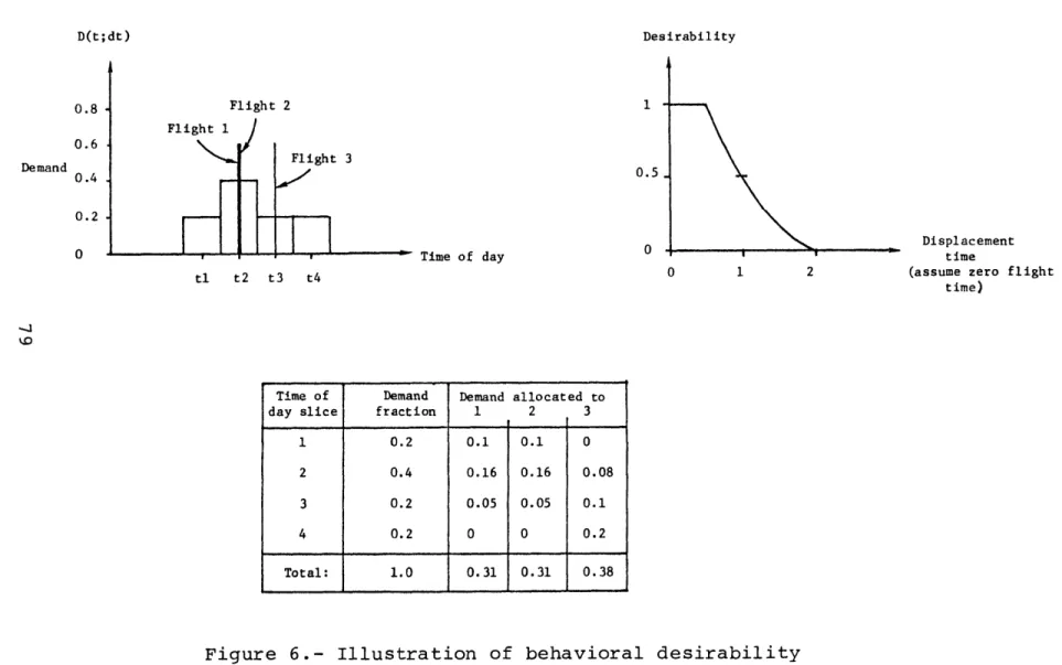
5 Behavioral desirability parameter function . . . . . . . 77
6 Illustration of Behavioral Desirability Parameter Computation. . . . . . . . . . . . . . . . . . . . . . . 79
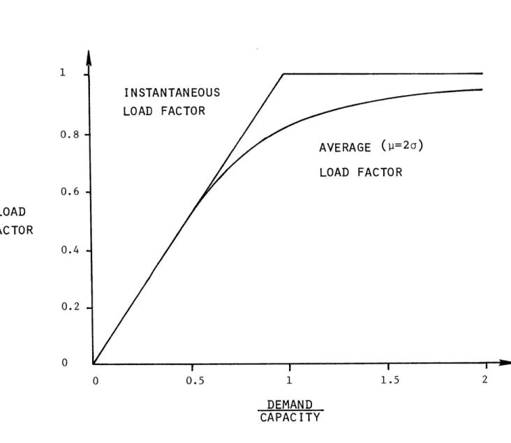
7 Load Factor Tail-off . . . . . . . . . . . . . . . . . . 84
8 Examples of non-iterative load buildup . . . . . . . . . 86
9 Example of iterative load buildup process . . . . . . . 90
10 Example of load factor tail-off simulation process . . . 93
11 Structure of game's software mechanization . . . . . . 114
12 Universe file listing for annotated example . . . . . 120
13 Sample interactive session with the participant file processor . . . . . . . . . . . . . . . . . . . . . . 122
14 OAG-type printout of flights offered by participants . 126 15 Total demand and initial desirability parameter determination. . . . . . . . . . . . . . . . . . . . . 128
16 Demand allocation process (iterations 1-6) . . . . . . 129
17 Demand allocation process (final results) . . . . . . 130
18 Traffic statistics printout for annotated example . . 136
20 Common data printout for participant "ZZ" . ... . 141 21 Game scenario geography and initial route structure for
MIT summer 1978 games . . . . . . . . . . . . . . . . 148 22 Schedules corresponding to lowest and highest value of
the level of service index . . . . . . . . . . . . . . 161 23 Variation of Level of Service index in game C's nine
largest markets . . . . . . . . . . . . . . . . . . . 163 24 Integration of gaming activity with corporate planning
activities . . . . . .... . . . .. .. .. .. 185 B1 Observed time-of-day variation of demand for Eastern
Airlines Boston-New York shuttle service . . . . . . . 213 B2 Departure/arrival desirability function derived from
observed data . . . . . . . . . . . . . . . . . . . . 217 B3 64-point Fourier Transform of raw desirability
function . . . . . . . . . . . . . . . . . . . . ... 218 B4 Evolution of time-of-day demand variation and
desirability function with harmonic filtering. . . . . 220 B5 Resulting time-of-day demand curves for various
departure-arrival time differences . . . . . . . . . . 221 Cl Statistical distribution of demand for a single flight 225 C2 Ideal and real average load factors vs. demand . . . . 227 Dl Participant File data structure . . . . . . . . . . . 230
D2 Universe file data structure . . . . . . . . . . . . . 233
D3 Simulation file data structure . . . . . . . . . . . . 236
TABLE
1 Participant's decision variables . . . . . . . . . . . 116 2 Run-time game parameters . . . . . . . . . . . . . . . 118
3 Aircraft data for MIT summer 1978 games . . . . . . . 146 4 Summer 1978 MIT games - system summary, initial state
and first iteration . . . . . . . . . . . . . . . . . 151 5 MIT summer 1978 games - system summary, second
iteration. . . . . . . . . . . . . . . . . . . . . . . 154 6 MIT summer 1978 games - system summary, third
iteration. . . . . . . . . . . . . . . . . . . . . . . 156 7 Average passengers/day carried in game C's nine larqest
markets . . . . . . . . . . . . . . . . . . . . . . . 158 8 Prices offered in the nine largest markets during game
C . . . . . . . . . . . . . . . . . . . . . . . . . . 159
9 Levels of service offered in the 9 largest markets
during game C. . . . . . . . . . . . . . . . . . . . . 160 10 Market shares on nine largest markets during game C . 164 11 Game "C" system analysis - revenues and costs . . . . 164
CHAPTER I
INTRODUCTION AND OVERVIEW
This chapter presents the motivation, goals and scope of this work, and an overview of the development and current use of games.
1.1 MOTIVATION OF WORK
The use of computer simulations to analyze large complex systems is now a well-established technique. By combining detailed numerical models of each component of the system, the behavior of the entire system can be simulated, observed, and
analyzed; some examples of systems that have been successfully designed and analyzed by means of computer simulations are communications networks, the Microwave Landing Systems (MLS)
that competed for the ICAO standard, and many aircraft and spacecraft, such as Apollo and the Space Transportation System
("Space Shuttle").
Attempts to simulate systems that involve human decision-making (pricipally economic and economy-related systems) have
not been so successful. The difficulty in modeling an indi-vidual's decision-making process: leads to the impossibility
of fully modeling such systems, short of including a human element in the simulation itself. This is precisely the
essence of the gaming approach to system simulation a number of "players" (properly called "game participants") drive, with
their decisions, numerical models of the other components of the system under consideration.
This effort is motivated by the author's belief that research on domestic air transportation may benefit from the use of such a game for the following reasons:
a) There is a significant number of mathematical models developed or in development about elements of its operations, which have not been
inte-grated.
b) The industry is reaching a turning point, namely deregulation, which increases the relative impor-tance of the human decision-making element over a wider range of options.
* Traditional microeconomic demand-supply equilibrium models, such as the Cournot solution, do not model the producer decision-making process; they simply postulate a certain behavior, and model the mathematical consequences of that behavior.
The effort undertaken in past years to develop and refine mathematical models for the airline industry, was made
possi-ble in part by the wealth of numerical data availapossi-ble. In their unique position between private industry and the public utilities, the airlines have been forced to keep and make pub-lic a staggering amount of data. The high technology environ-ment that permeates the industry has enhanced both the
quan-tity and quality of this data gathering effort, and the uses of this data for model-building (and analytical) purposes.
These models are highly interrelated, but in general are used individually by making simple assumptions about other elements of the system. Thus, sophisticated demand models assume simple statistical supply functions, supply models assume non-competitive environments, etc. A computer simula-tion, such as the one required for this game, seems to be the ideal way of integrating many of these models in a coherent fashion, while the gaming dimension acts as a surrogate for the unmodelable human decision-making component.
One of the consequences of the current trend towards der-egulation in the air transportation industry is an increase in
the freedom and range of management decisions. This in turn increases the relative importance of the human decision-making element in the total environmental uncertainty in which the industry must operate. The difficulty in modeling the indi-vidual decision-making process indicates a gaming approach to systems analysis.
1.2 GOAL AND SCOPE OF THIS WORK
With the above motivation in mind, we define the goal of the present effort as follows:
To design, build, and test a computer game for U.S. domestic passenger air carriers, based prima-rily on existing mathematical models of its opera-tions and economics. This game must offer a suffi-cient degree of quantitative accuracy to analyze effects of managerial and regulatory decisions on an air transportation system. As a secondary goal, the game should also be usable as a training device in
the teaching of subjects on air transoortation.
We also impose the following limitations: W i NMIOMM
1.- New models are not built, unless found
absolutely indispensable for the simulation's accuracy or completeness. In this context, and
in the rest of this work, the word "model" shall be used to denote mathematical models of the
var-ious functions that make up the game's environ-ment simulation (e.g. the demand model, the cost of money model).
2.- Similarly, the numerical data (parameters) that the models may require, are not developed. Maxi-mum use is made of existing data, and deficien-cies in the data available are pointed out but not corrected.
3.- Only test and demonstration cases are run. The application of the game to the analysis of real-world problems or situations is left as future work to be done.
1.3 APPROACH USED
A computerized game is actually made up of two compo-nents:
a) A set of rules and data that define the "game scenario".
b) The computer model of the system under considera-tion.
The purpose of the game scenario is threefold:
a) To define and limit the decision-making freedom of the participants (e.g. degree of price
compe-tition, route structures, etc.)
b) To define the environmental assumptions under which a particular game is run (e.g. types of aircraft, market demand parameters, etc.)
c) To model aspects of the environment for which there are no convenient mathematical models suit-able for computer coding (e.g. when and to whom government subsidies are paid).
Throughout the work, the term "environment" or "game environment" will be used to denote the collection of data and processes external to the system but which affect the behavior of the system. In our case, the "system" is made up of a
num-ber of airlines, and the environment is made out of elements such as the latitudes and longitudes of airports (physical environment), the speed and fuel consumption of aircraft
(technical environment) or the route freedom of the partici-pants (regulatory environment).
The allocation of system and environment models to either the computer simulation or the game scenario is one of the important design decisions to be made. The computer simula-tion offers greater data-processing capability at the expense of flexibility (every possible case must be pre-programmed). The scenario rules offer greater flexibility, but must not require tedious calculations. In addition, only well-defina-ble models can be mechanized as computer code, whereas the
scenario rules may use subjective judgement ("umpiring").
This work has proceeded in the following fashion:
a) The functional structure of the game was defined.
b) The level of detail at which the game was to be implemented was determined.
c) Based on this level of detail, a selection of which components of airline operations to be
included was made. These components were then allocated either to the computer simulation or to the scenario rules.
d) The mathematical models for the components of the computer simulation were defined.
e) The models were implemented (coded), along with the additional software required to mechanize the game.
f) The integrated game was tested with simple cases to test the validity of the code.
The next Section reviews the history and development of games, in particular computer games. For readers not familiar with the peculiarities of the airline industry, Appendix A describes briefly the principal aspects of air transportation economics that influence this work. Chapter II describes the game design process, the tradeoffs involved, and the design decisions made (steps a and b, above). Chapter III explains
simula-tion. Chapter IV includes a description of the software implementation of the game, a detailed, annotated example illustrating the functioning of the mathematical models used, and a sample of actual use of the game for teaching and analy-sis purposes. Chapter V discusses a number of extensions and improvements that have been identified during the game's
development, as well as some suggestions for possible applica-tions of the game. Chapter VI summarizes the conclusions and recommendations for future work. Appendices B and C contain a detailed development of the demand vs. time-of-day function and the load factor tail-off function respectively. Appendix D contains a full description of the data bases used, along with the conversational commands available to interactively access, modify or update these data bases.
1.4 ORIGIN AND DEVELOPMENT OF SIMULATION GAMES
Games, that is, physical or mental competitions between two or more participants carried out according to a set of rules, are probably as old as mankind; a bas-relief in the palace of Ramses II (1292-1225 B.C.) in Thebes shows the King playing a board game with pieces that bear an astonishing
(as opposed to most physical games, or "sports") mimic more or less accurately a real-world situation; when they do, they are called "simulation" games.
Traditionally, simulation games have been directed towards the warfare-making activity of mankind; they ranged from table-top board games in which tokens idealize, both in shape and in function, various elements of an army to, at the other extreme, full-sized maneuvers in the field complete with mock battles. From the very beginning a tradeoff between cost and realism becomes evident: the more realistic the simula-tion, the more expensive it is to run ("play") the game.
The original purpose of these games seems invariably to have been that of providing the participants with vicarious experience in the decision-making process of the simulated situation. With the passing of time, the low-cost end of the spectrum evolved into less realistic (and less useful) but more enjoyable forms designed for pleasure, not training.
Simultaneously, the high-fidelity end evolved into various forms of military gymnastics (the medieval jousts and tourna-ments, and the XVIIIth century army drills) with little or no decision-making contents.
It is only in the XVIIIth century, particularly in the central european army staffs and staff schools, that the value of games as decision-making training devices is formally rec-ognized. Prussia's Baron von Peisswitz, and his son Johann, are generally credited by military historians with the devel-opment of the first modern war qame, or Kriegspiel, around 1811. This game, played on maps or sand-table models of a battleground, was made up of rules determining the outcome of engagements between different types of military units
(fusili-ers, cavalry, etc.). Its purpose was twofold: to provide
officers with simulated field command experience, and to expe-riment with unconventional combat tactics. For the first
time, the game environment is analyzed rationally for the pur-pose of developing detailed and realistic models, including effect of terrain and weather, casualties inflicted, etc. Again, the realism-cost tradeoff is in evidence: umpires were usually needed to evaluate the results, both in order to reduce the burden on the participants and because some of the models used involved some form of subjective judgement.
Up to this stage in the historical development of gaming, simulation of the real environment is performed by a set of manually-evaluated rules or "models" describing the effects of
process of evaluating these rules is traditionally called "scoring". The advent of digital computers radically reduced the cost of scoring to an extent such that the degree of
fidelity of the environment simulation is now the availabil-ity, applicabilavailabil-ity, and accuracy of the models themselves. The tradeoff between realism and the cost of gaming to the player still exists, because high model fidelity usually
requires a larger number of decisions and more input data from the game players than lower-fidelity games.
The emergence, towards the end of World War II, of the mathematical discipline called "Operations Research" gave
impetus to the search of rational, analytical, decision making processes. It was soon found, however, that only a limited
number of decision-making situations were solvable by pure analytical techniques. Ellis A. Johnson, head of the Naval Ordnance Laboratory (NOL) Operations Research group approached
the problem of selecting mining patterns by playing games
between minelaying and minesweeping teams. The mining strate-gies thus developed actually improved the effectiveness of mining operations agains Japan.
In early 1950, George Gamow, at John Hopkins University Operations Research Office (ORO) developed "TIN SOLDIER",
which is recognized as the first game designed specifically as a mathematical model for use in analytical research (Reference
1). The use of stochastic processes in that game lead to the introduction of a computer for scoring via Monte-Carlo techni-ques (an IBM 650 was expressely installed at ORO to run the game), and by 1952, ORO had the first full-scale
computer-scored game. By 1962, it was estimated that 57 organizations in the U.S., 2 in England, and one in Canada, used games for one purpose or another. Of these, 5 were primarily oriented towards training, 16 towards the evaluation of military opera-tions at different levels, and 47 devoted to research and
development.
In 1956, an American Management Association (AMA) team, with the cooperation of IBM, was set up to develop a manage-ment game following closely the military models. A
well-pub-licized demonstration was set up at the New York headquarters of the Association, with twenty corporation presidents partic-ipating in it. Reactions to it ranged from outright enthusi-asm to severe skepticism (Reference 2). After this initial attempt, business interest in games dwindled, partly as a con-sequence of the reaction to the cultural disruption caused by the introduction of computers in general, partly because of the lack of the required analytical and mathematical modeling expertise in the industries themselves.
The academic community, however, soon grasped the poten-tial that such games could have as training tools. In addi-tion, they had the expertise in modeling the various compo-nents of the business environment that computer experts
lacked. The result was a veritable boom of "Management Games" designed as low-cost, high-realism class exercises for manage-ment students. From the first UCLA game, with only 8 decision variables, we now find games with more than 300 possible deci-sion inputs, and practically every management school in the country has at least one game implemented in its computer
sys-tem (Reference 3).
Some authors define "operational games" as those games where the environment modeling is accurate and realistic enough to allow evaluation of operational decisions, whereas
the term "management games" is reserved to games designed with educational objectives in mind. Using this terminology, most military games are operational games. Academic, or management games proper, are usually classified as general purpose games
("general games"), and specific games.
General games are games whose input (decision) variables cover a wide range of managerial disciplines (production,
,Ow-Nw , I
finances, marketing, etc). The main purpose of these games is to show to the student the interrelationships between these various aspects of management (Reference 4).
On the other hand, games can be "specific" in one of two ways, which are sometimes found simultaneously:
- Discipline-specific: one aspect of the management skills spectrum is emphasized (marketing,
finance), while the others are eliminated or de-emphasized. Such games are usually designed for use in advanced courses in that subject (Refer-ence 5).
- Industry-specific: the idiosyncrasies of a par-ticular industry (e.g. the Oil industry) are emphasized (Reference 6).
As it turns out, most industry-specific games are also discipline-specific.
In the field of air transportation, there are three gam-ing efforts known to the author. The first, by Air Canada
decision variables (inputs) include the number of flights (but not their schedule), the aircraft's seating arrangement split
(first class/economy class), financial (two alternatives), maintenance procedures, and passenger service, advertising and market research expenditures. The game is designed for train-ing airline personnel, and specifically to show the interrela-tionships among the various departments of the airline.
The second, at the University of Tennessee College of Business Administration, is non-interactive (a participant's actions do not affect the othr participant's results), and contains some probabilistic elements. As listed in the avail-able literature, this game's decision variavail-ables include
routes, aircraft type and configuration, arrival times (sic), advertising policy for each city, and market information to be purchased. The training ourpose is to "improve the decision-making process, reactions, goal selection, and implementation"
(Reference 3).
The third, by H. B. Tyber at McDonnell Douglas (Reference 8) simulates a multi-carrier (up to five participants) airline system at the senior management level. Decision variables are: total number of flights in each one of four regions (e.g. "the North Atlantic"), crew wage levels, short-term borrowing
level, and the inevitable advertising and market research expenditures. Certain number of "frills" (e.g. the relative effect of on-board movies vs. that of free drinks) are added in for realism. This game was designed for use in a corporate Market Development Course to "provide airline employees with a
review of all the aspects of airline planning on a systems-wide basis".
All three games described are typical business-school marketing-oriented games mechanized in the framework of the air transportation industry. These games, and in particular the level of detail and quantitative accuracy of their envi-ronment models, were designed solely for training purposes, and are not suitable for analysis, research, or "operational" uses.
CHAPTER II
GAME DESIGN
This chapter analyzes the overall game design, the allo-cation of elements of the game to either the computer simula-tion or the scenario rules, and the different levels of detail at which the environment can be simulated. The decisions
made, and the rationale behind these decisions are described.
2.1 OVERALL GAME STRUCTURE
In the most general terms, a game functions in the manner shown schematically in Figure 1. There are N participants
("players"), each representing a competing operational unit (in our case, air carriers). Each participant produces a set of "decision variables". These variables, plus whatever scen-ario data is applicable, constitute the input to a simulation of a real-world situation, in our case, the operations of domestic air carriers. The output of the simulation is data which can be grouped according to its purpose:
Common data
p
System data
Figure l.- Generalized game structure
a) Data of interest to the game user for the purpose for which the game is performed. We call this
"System Analysis" data.
b) Data which is made available to all participants ("Common" data).
c) Data which is made available to each participant on an individual basis ("Private" data).
The game is carried out as a sequence of plays, or "iter-ations". Each iteration corresponds to the simulation of a certain amount of real time, such as a month, a quarter, or a year. Thus, the participant's decisions are fixed during that simulated time, and the simulated results represent the aver-age results over that same period of time. Participants are allowed to change their inputs (and examine the data made available to them) between iterations. Data available to the participants include the above-mentioned "Common" and
"Pri-vate" data, scenario data, and, if allowed by the scenario rules, communications between participants.
The scenario, which includes both rules and all the mod-els and data not internal to the computer simulation, may be
static or change from iteration to iteration ("dynamic scen-ario"). In particular, the scenario changes may be keyed to the results of the simulation via some feedback data. If human decision-making is part of this feedback, then we have in
effect an (N+l)th player (the "exogenous participant"), or an umpire.
Of particular interest is the start-up (first iteration) problem, since the only data available to the participants is
the scenario data. There are several ways in which the game may be initiated. Two possibilities are:
a) The scenario may depict a real-world startup sit-uation (e.g. the creation of a new carrier
oper-ating in a new market).
b) The scenario data may include simulated past-op-erations Common and Private data.
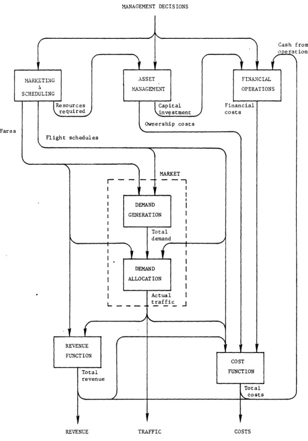
Figure 2 shows, in schematic form, a model for an air carrier, in terms of the flow of orocesses and data that link operational results to the management decisions. The central process in this flow is the determination of total demand and
the allocation of this demand among competing carriers (and
MANAGEMENT DECISIONS Fares Flight schedules MARKET SDEMAND GENERATION Total demand DEMAND ALLOCATION * Actual L ... . ... t r af fic REVENUE T FCTS FUNCTION COST Total FUNCTION revenue Total .costs
REVENUE TRAFFIC COSTS
among a carrier's different flights). Total demand and its allocation are influenced by management's decision of the level of service offered by the flight schedule the price of this service. The level of service (schedule) also determines the resources (aircraft, ground facilities, flight crews,
etc.) required to provide these services.
The resources required then determine the cash flow required (investment). These financial requirements have a certain cost associated with them; costs are also associated with the maintenance and use of the resources, as well as
other operational requirements of providing the level of serv-ice determined by the management. Costs combine then with the revenues (intenal and external) to yeld the carrier's net
income. This net income (positive or negative) in turn affects the financial cash flow.
2.2 DESIGN DECISIONS AND TRADEOFFS
The three games described in Section 1.1 do not meet the level of detail and numerical accuracy required of an opera-tional game for two reasons: first, they do not attempt to
model in detail the actual operations of airlines; second, the range of operating conditions that they are capable of simu-lating is limited to the "usual" conditions that have pre-vailed in the industry during the past two decades.
Previous efforts at modeling in detail the operation of airlines (mostly directed towards operational analysis, not gaming) also have made use of this historical limited
opera-tional freedom. For example, the McDonnell-Douglas ASPEM (Airline Schedule Planning and Evaluation Model, References 9 and 10) and the Boeing SSFX (Reference 11) assume a fixed demand and a fixed market share (oer market) irregardless of
the simulated carrier's operations. This assumption may have been acceptable during the CAB-regulated market years, but is certainly not valid in a deregulated competitive scenario. The same observation applies to the traditional "Market
Share=Frequency Share" model. In view of the limitations of these previous efforts, design of the game has to be started from scratch.
In order to design the structure of the game and its sim-ulation, three basic decisions must be made:
a) The level of of detail (or aggregation) at which operations will be simulated
b) Which elements of operations to include in the game, and which to ignore or simplify.
c) Which elements to mechanize as computer code and which to be considered part of the scenario
rules.
These decisions interrelate, e.g. whether to include a model for certain operational element depends on whether the
level of aggregation used makes that element irrelevant, optional, or necessary for the rest of the simulation.
These decisions were also affected by limits on the resources available to the author for implementing of the
game. Elements or models excluded or simplified for cost rea-sons are identified as such, and suggestions for their incor-poration or improvement given the necessary resources, are
2.3 ALTERNATIVE LEVELS OF AGGREGATION
We can identify three broad levels of aggregation at which the game and its environment simulation can be imple-mented. These levels of aggregation are examined as they
affect the modeling of demand, supply, market share alloca-tion, and costs. We also identify the costs and benefits of each level of aggregation on these components.
2.3.1 System-wide aggregation
At this, the topmost level of aggregation, supply and demand are determined as aggregates over an entire market area, such as "the North Atlantic" or "the transcontinental markets". Supply is determined by the number of flights offered in that market, while demand is a function of the
total supply, and perhaps an average fare level. Market share is determined from the flight share (a proxy for frequency share, since the average number of flight hours per flight is the same for all the carriers in the area), with perhaps some provision for differential area-wide fare levels.
The operating costs, at this level of aggregation, are usually assumed to be proportional to the number of flights, based on average costs, with perhaps some provision for econo-mies (or diseconoecono-mies) of scale. With this crude structure, the efficiency of each carrier in the use of resources cannot be determined from the participant's decision variables, and must be set externally (e.g. the same for all participants). In other words, costs are determined solely by the aggregate level of service offered.
The advantage of this level of aggregation is the sim-plicity of the participant's decision variables required to model the carrier's management. Indeed, at this level, it would be feasible to construct a mathematical model for these decisions, thus eliminating the human element and converting
the game into a numerically-solved, closed form analysis model.
System-wide aggregation has been used, and is very appro-priate to management training games, where fidelity in
model-ing the operational aspects of the industry is secondary to the goal of offering the participants a subjective "feel" for what it is like to be the Chief Executive Officer of an
air-line. An example of this level of modeling is the McDonnell Douglas (Peference 8) game already mentioned.
35 AW-1
1
2.3.2 Market-level disaggregation
At this level, each individual market (i.e. origin-desti-nation demand area pairs) is modeled. This requires the mod-eling of individual flight itineraries if any network effects are to be observable. In addition, the user may assign indi-vidual aircraft types to indiindi-vidual routes. This in turn allows estimation of flight-dependent direct operating costs. Since the timetable of departures is not modeled, there is no way of determining either the exact number of aircraft
required to fly the entire network, or the relative desirabil-ity of otherwise identical flights. Rough approximations to the number of aircraft needed can be obtained by dividing the total number of flight-hours implied by the itineraries by an average utilization. Since different aircraft types can be assigned to each itinerary, the fleet requirements and owner-ship costs can be evaluated by aircraft type.
Now it is possible to model both regulatory restrictions on routes, and the effect of differential fares. The number of decision variables that the user must now input is signifi-cant (flight itineraries, aircraft used on each itinerary, fares). Acquisition, sale, and lease of individual aircraft
types can be modeled at this level, but with limited useful-ness, since the exact number required cannot be determined.
The Air Canada and University of Tennessee games men-tioned in the previous chapter are examples of this level of detail.
2.3.3 Schedule-level disaggregation
At this level, the schedule (time of day) of departure for each flight is also specified. This allows aircraft flow to be modeled, and hence the exact size of the fleet required can be determined. This in turns allows the use of a detailed model of aircraft acquisitions and transactions, including depreciation costs, tax rebates, etc. On the demand side, the time-of-day variation of demand (and flight preference) must be modeled. The added demand generated by connecting services can be included.
Direct and indirect operating costs are modeled in the same way as in the previous level; maintenance and crew costs must be averaged over the flight-hour.
The cost of this additional level of detail is, of
of the participant, at least until an acceptable computer model of the scheduling function of an airline can be designed.
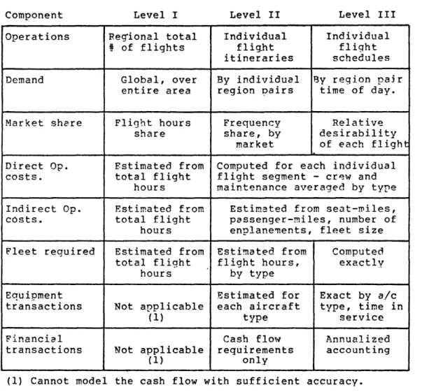
These three levels of aggregation, also referred to as "Level I", "Level II", and "Level III", and their effect on some of the components of the system are summarized in Figure 3.
The highest level of aggregation, systemwide, was not deemed acceptable for the type of gaming that was sought.
Although usable for training purposes, it does not model real-ity with any degree of precision required to perform any use-ful experimentation.
The next level, dissagregation by market, is detailed enough to perform some experimentation, e.g. differential fares, deregulation of routes, elimination of cross-subsidiza-tion, etc. It was originally thought to be the ideal level to start this simulation project, since it has a very simple user interface (flight itineraries and equipment only). However, it lacks the capability of accounting for the financial
Operations Regional total Individual Individual
# of flights flig.ht flight
itineraries schedules
Demand Global, over By individual By region pair
entire area region pairs time of day.
Market share Flight hours Frequency Relative
share share, by desirability
market of each flight
Direct Op. Estimated from Computed for each individual
costs. total flight flight segment - crew and
hours maintenance averaged by type Indirect Op. Estimated from Estimated from seat-miles,
costs. total flight passenger-miles, number of
hours enplanements, fleet size
Fleet required Estimated from Estimated from Computed total flight flight hours, exactly
hours by type
Equipment Estimated for Exact by a/c
transactions Not applicable each aircraft type, time in
(1) type service
Financial Cash flow Annualized
transactions Not applicable requirements accounting
(1) only
(1) Cannot model the cash flow with sufficient accuracy.
Figure 3.- Possible levels of model aggregation
and their effect on several system components.
39
Financial planning was the reason why the third level, disaggregation by schedules, was selected. Coupled with
rea-sonable scenarios for cost of money and equipment, it allows experiments of a reasonably long time frame (several years), that is, strategic planning, to be carried out.
2.4 SELECTION AND LIMITATION OF COMPONENTS
Real-world air carrier operations have a large amount of variability: airlines carry oassengers (in two, now sometimes three service classes), mail, cargo, charging wildly disparate fares, and sometimes generating revenue from non-flying opera-tions, such as leasing out their equipment, or embarking in "peripheral" business, such as training other carrier's flight crews, providing catering services, or running hotel chains.
It is impractical to include in the game every possible operating and revenue-generating activity, cost element, etc.
In addition, the structure and level of detail of the game inherently limit the level of detail of the game's components
(e.g. the structure of the cost model). In this section, we discuss five elements of the game, namely demand, supply, the asset and financial management function, and the cost and
rev-enue structures. The real-world components of each of these elements, its variability, and the limitations and
simplifica-tions that will be used in this game are discussed.
2.4.1 Comoonents of Demand
There are several kinds of "goods" that may require air transportation: passengers, freight, mail. Under certain cir-cumstances these demands do not compete for the available sup-ply (e.g. belly cargo on a passenger flight). In most cases, however, there is a certain degree of interaction (e.g. pay-load tradeoff between cargo and passengers on a convertible aircraft, or network scheduling conflicts between freight and passenger service). More evident is the competition for
serv-ices of different "grades" of the same type of demand, such as business passengers and pleasure passengers, which share the same supply of seats.
The simulation of multiple, simultaneous, interactive demands requires separate modeling (each with its own parame-ters) of each demand. In addition, separate supply parameters must be determined for each demand (e.g. fares, the number of first-class seats vs. number of coach seats or passenger-cargo tradeoffs for each aircraft, etc). This results in a large
effort being required both to play the game and to prepare it (the number of market demand parameters and of decision varia-bles is multiplied by the number of different demands that are simulated).
Admittedly, there are problems that can only be analyzed using multiple demand. However, within the scope of this effort, we can obtain useful results from the simulation of a
single class of demand, such as a single class of passengers or a single class of freight. Section 5.1 discusses how the game can be extended to the case of multiple interacting demands.
Even for a single class of demand, we still must deter-mine what endogenous and/or external variables will affect
this demand. In the real world, total demand changes with time: time of day, day of the week, season of the year. Since we are going to restrict flights to daily frequency, there is
no benefit from modeling the day of the week dependence of demand. On the other hand, we will be modeling flight depar-ture and arrival times, so that the time-of-day variation of demand must be modeled. Seasonal variations affect the
results if the period simulated per game iteration (iteration period) is of the order of the seasonal variation (around
three months). Seasonal variation of demand can thus be mod-eled by simply changing market demand parameters from one game iteration to the next.
Since one of the objectives of this game is to allow sim-ulation of de-regulated, competitive scenarios, we must
include the effect of price on total demand, as well as the effects of competitive services and prices on the allocation of total demand.
2.4.2 Components of Supply
At the level of detail selected, each game participant must specify each flight in his network. The word "flight" is sometimes used to denote two different concepts:
a) The movement of an aircraft through a series of airports ("flight itinerary") carrying
fly-through passenqers (e.g. "Flight 365" is a flight from 30 to NYC to DCA).
b) The air transportation service offered between two cities (e.g. "Flight 365 between BOS and NYC", "Flight 365 between BOS and DCA" and
"Flight 365 between NYC and DCA" for the same BOS-NYC-DCA flight).
In this work we will reserve the word "flight" to signify the first meaning, i.e. "Flight 365". We will use the terms
"service" or "service offering" to signify meaning b) above. Thus an N-segment flight (in our meaning) will produce
(N+1)N/2 service offerings. Conversely, a service offering may require more than one flight (a connection). Service
offerings (not "flights") may be non-stop, n-stop, or connect-ing. Thus, the Official Airline Guide (OAG) is properly a listing of service offerings, rather than of flights.
Flight itineraries and schedules change, in the real world, in two different periods:
a) The regular, published, day to day variations, such as a flight not offered on Sundays, or a weekly itinerary alteration.
b) The monthly (or discrete) readjustment of the schedule for marketing reasons (e.g.
seasonal-ity), which is reflected in a new edition of the OAG.
In order to model weekly schedules, each day of the week must be simulated and processed separately for each game
iter-ation. The simple expedient of multiplying each flight's demand by its relative frequency (e.g. 2/7 for a twice-weekly flight) does not produce valid results at the level of detail that we are using. To illustrate this, consider a market with one daily flight and two twice-a-week fliqhts. All other
flight parameters being eaual, the simple frequency weighting mentioned above would distribute 63.6% (7/11) of the demand to the daily flight, and 18.2% (2/11) to each of the twice-weekly flights. In reality, this proportion depends on whether the days of the twice-weekly flights coincide or not.
If indeed they do, we have two days of the week with three flights, and five days with a flight each. We would thus expect that the daily flight would get 5/7 of the demand for the five days in which it is the only flight, plus 2/21 for the two days during which it has to share the demand with two other flights, for a total of 80.9% of the market. The two twice-weekly flights would get only 2/21 (9.5%) of the market each.
Thus, in order to simulate the effects of weekly varia-tion of supply, we must simulate each day of the week sepa-rately (maybe with varying demand, as mentioned in the previ-ous Subsection), including input data with each flight to
allow determination of the exact schedule for each day of the week. We have decided that the complexity of input data and increase in computation time is not cost effective for
domes-* tic airlines*.
The second, monthly or seasonal variability, is taken care of, and is limited in freguency by, the simulated length of each game play or iteration. This length is left variable, and is determined by the parameter NDP (Number of Days per Period). Thus, depending on the objectives of the particular game run, weekly, monthly, quarterly or yearly variations can be introduced. We have elected to ignore non-scheduled opera-tions (e.g. individual charters). The extension of an itera-tive game such as this to include non-repetiitera-tive events such as a charter flight is a major challenge.
The process of converting flight itineraries and sched-ules into a list of service offerings such as the OAG requires two steps:
a) Conversion of multiple-segment flights into a list of individual direct-service offerings.
* This may be required for the simulation of long-haul inter-national operations, where weekly rather than daily sched-ules are the rule.
b) Linking of direct-service offerings into connecting-service offerings.
There is a one-to-one correspondence between single-seg-ment flights and their corresponding direct non-stop service offerings, but multi-segment flights may generate direct serv-ice entries in the offerings lists of many airport pairs.
Manual conversion from one form to the other would impose an enormous burden to the game users. We thus find it mandatory to have the computer perform this function.
It would also be highly desirable to have the computer perform automatic connection generation. There are several algorithms published that will perform this function (e.g. Reference 10)*. Again, economic limitations have prevented the implementation of an automatic connection generator, and participants are reauested to identify all connecting service offerings they wish to supply. Computer code has been pro-vided, however, to aid the user in determining the physical validity of such connections (e.g. sufficient connecting time at the connecting airport).
*The problem of how to generalize the allocation of revenue in an interline connection remains to be solved.
Thus, the participant specifies an input list of flight itineraries with scheduled departure times and, in an interac-tive conversational mode with the computer, gets a listing of direct services by market, from which a list of connecting
services can be constructed with computer assistance.
2.4.3 Components of Asset and Financial Management "Management" of assets and cash involves the determina-tion of the assets (and cash) required to supply the services represented by the participant's schedule, and the determina-tion of the transacdetermina-tions required to secure such assets and cash.
The only non-cash assets that will be modeled explicitly are aircraft. All other resources necessary to run an airline
(e.g. ground facilities, reservation system computers, etc.) will not be explicitly modeled. Its costs will have to be
aggregated to other measures of activity that somehow reflect the use of these resources, such as number of passengers
enplaned or total number of aircraft block-hours (see "compo-nents of cost", below).
The minimum flight equipment needs are automaticaly com-puted from the participant-specified fliqht schedule. This minimum can then be compared with the equipment available to the participant as a result of his equipment transactions. However, what action to take in case they don't match is left as part of the individual aame's scenario rules (e.g. force an automatic lease of the reauired aircraft). Also, the scenario may require a fixed percentage of spare aircraft of each type.
The number and variety of forms that asset acquisition and disposition may take (e.g. sales, purchases and leases for
aircraft, bonds, stocks, notes, for cash) makes it quite
impractical to attempt to build a complete computer model that would cover all, or even most, of the real-world possibili-ties. Modeling of these transactions requires two different types of data processing:
a) The data processing associated with the determi-nation of certain parameters of the transaction, such as the interest at which a participant can borrow money in the short-term or the current selling price of a used aircraft.
b) The accounting of the cash flow consequences of the transactions actually carried out by the game participants.
The amount of data processing required for the first pur-pose is moderate, and can be carried out manually (e.g. as a
table of interest rates vs. the firm's Debt/Equity ratio). The accounting process, however, can be tedious, and since the
computer simulation is performing the total accounting for each participant, we have decided to include the cash flow resulting from all transactions in the computer simulaton. This split requires that some data be exchanged between the
game scenario rules and the simulation, as shown in the dia-gram of Figure 1. Chapter IV describes how this communication is mechanized (via the so-called "simulation file").
A restriction curently placed on the financial transac-tions is that they do not have periodic repayments of princi-pal (e.g. mortgages). This is due to the structure of the communications data between the game scenario and the simula-tion. This restriction should be removed in subsequent game improvements.
2.4.4 Components of Revenue
In the strict financial accounting sense, all revenue produced by a company under normal circumstances is considered
"operating revenue" irregardless of its source. We will, how-ever, use this term to denote the revenue originated by the
fare charged to each passenger (or ton of freight) actually carried. Non-operating revenues then include government
sub-sidies (which may in fact depend on the services supplied), the results of resource management (e.g. sale of assets) and the results of other activities, such as crew training or non-flying business.
Without demeaning the importance that income from these peripheral activities may have in real-world air carriers, we find them outside the scope of our interest, (air transporta-tion), and thus will not consider them in the game. Govern-ment subsidies will be considered as oart of an individual game's scenario as required, since its modeling does not
require extensive data processing, and since the great variety of forms they may take defies its being programmed as computer code.
As in the case of financial transactions, the details of specific asset transactions will be modeled by scenario param-eters (e.g. market prices of aircraft and short-term interest rate) although its cash flow effect, as with subsidies, will be taken into consideration by the computerized participant
financial accounting process.
There is still the basic revenue from fares; in the real world, the fare structure is quite complicated, and, under the current deregulatory trend, is becoming more and more so.
Since we are not currently modeling multiple classes of demand (e.g. business vs. pleasure travellers), there is no possibil-ity of including multiple fares based on the class of service
(e.g. first, coach) in the game. On the other hand, it would be easy to extend the fare structure based on the time of day of the flight and the type of equipment used. However, we have opted not to include it in this game mechanization, again due to resource limitations. It is our claim that useful
results may be obtained even with single fares ("average yield") for each city-pair, as long as each participant may select its own yields*.
* The average yield per passenger on a city pair is defined as the total revenue divided by the number of passengers, thus averaging over all types of tariffs (day, night, excursion, APEX, etc.)
2.4.5 Components of Cost
In our generalized model of air carrier operations (Fig-ure 2), we can identify three sources of costs: asset manage-ment costs, financial costs, and operational costs.
Asset management costs include the cost of acquiring, keeping, and disposing of non-cash assets, limited in our case to flight equipment. Some examples of this cost are the
depreciation of owned flight equipment, the lease payments for leased equipment, and aircraft insurance. This cost may be
"negative", such as when an owned aircraft is leased out.
Note that the expenditure required to buy an aircraft is not a cost.
Financial costs include the cost of acquiring the cash needed to balance the firm's cash flow requirements. Again, this cost can be negative (as when the interest from the investment of excess cash exceeds the interest of the out-standing debt).
Operations cost is simply "everything else". In our
scheme, we make it a function of the schedule, the total traf-fic, and the total revenue. Our cost structure is directly
tied in to the measures of activity that are generated by the simulation: block hours (for each aircraft), departures, pas-sengers carried, etc. This structure is described in detail in Section 3.6. Note that the traditional classification of costs as "direct" and "indirect", while of great analytical significance, is of little use for modeling purposes at this level of detail.
A further element of "cost" are the taxes levied on the participant airlines. The structure of real-world fiscal laws
is so complex and ever-changing, that it is not realistic to attempt to model the exact taxation mechanism. We have
decided to include in this game three components of taxes:
a) A simple corporate income tax rate. b) A simple capital gains tax rate.
c) An accumulative credit due to the Investment Tax Credit (ITC), again made up of a simple rate.
The three rates can, of course, change during the game, as part of a dynamic scenario. A problem unique to this par-ticular "cost" is that in the real world it is a function of the net income over a very specific span of time (the "fiscal year"). Unless the simulation period coincides exactly with the fiscal year, we must adopt one of two solutions:
a) Prorate the (annual) tax liability over each sim-ulation period, based on the period's income.
b) Compute this expenditure only on those qame iter-ations coinciding with the end of the fiscal
year.
The first approach has the disadvantage of overestimating taxes (profitable and unprofitable periods cannot be averaged out during the year). The second approach complicates the structure and use of the game (more past history must be saved, the results depend on the position in the fiscal cycle of the period being simulated). We have selected the first solution: taxes are computed every game iteration as if the fiscal period was exactly one game period.
CHAPTER III
MODELS USED IN THE COMPUTER SIMULATION
This chapter describes the mathematical models used in the game's computer simulation. These models must perform the following functions during each iteration:
a) Transform the supply data from the participant's format to a format compatible with that of the demand function.
b) Determine total demand by market.
c) Allocate the demand and the revenue it produces among the participant airlines.
d) Determine a number of cash flow elements, such as total revenue, costs, etc. for each participant
(accounting function) and collect and summarize system data (performance reporting function).
The software implementation of the computer simulation is overviewed in the next chapter.