HAL Id: hal-00298398
https://hal.archives-ouvertes.fr/hal-00298398
Submitted on 10 Jul 2006HAL is a multi-disciplinary open access
archive for the deposit and dissemination of sci-entific research documents, whether they are pub-lished or not. The documents may come from teaching and research institutions in France or abroad, or from public or private research centers.
L’archive ouverte pluridisciplinaire HAL, est destinée au dépôt et à la diffusion de documents scientifiques de niveau recherche, publiés ou non, émanant des établissements d’enseignement et de recherche français ou étrangers, des laboratoires publics ou privés.
Results from the implementation of the elastic viscous
plastic sea ice rheology in HadCM3
W. Connolley, A. Keen, A. Mclaren
To cite this version:
W. Connolley, A. Keen, A. Mclaren. Results from the implementation of the elastic viscous plastic sea ice rheology in HadCM3. Ocean Science Discussions, European Geosciences Union, 2006, 3 (4), pp.777-803. �hal-00298398�
OSD
3, 777–803, 2006Implementation of elastic viscous plastic sea ice in
HadCM3 W. Connolley et al. Title Page Abstract Introduction Conclusions References Tables Figures J I J I Back Close
Full Screen / Esc
Printer-friendly Version Interactive Discussion
Ocean Sci. Discuss., 3, 777–803, 2006 www.ocean-sci-discuss.net/3/777/2006/ © Author(s) 2006. This work is licensed under a Creative Commons License.
Ocean Science Discussions
Papers published in Ocean Science Discussions are under open-access review for the journal Ocean Science
Results from the implementation of the
elastic viscous plastic sea ice rheology in
HadCM3
W. Connolley1, A. Keen2, and A. McLaren2
1
British Antarctic Survey, High Cross, Madingley Road, Cambridge, CB3 0ET, UK
2Met Office Hadley Centre for Climate Prediction and Research, FitzRoy Road, Exeter, EX1
3PB, UK
Received: 13 June 2006 – Accepted: 19 June 2006 – Published: 10 July 2006 Correspondence to: W. Connolley ([email protected])
OSD
3, 777–803, 2006Implementation of elastic viscous plastic sea ice in
HadCM3 W. Connolley et al. Title Page Abstract Introduction Conclusions References Tables Figures J I J I Back Close
Full Screen / Esc
Printer-friendly Version Interactive Discussion
Abstract
We present results of an implementation of the Elastic Viscous Plastic (EVP) sea ice dynamics scheme into the Hadley Centre coupled ocean-atmosphere climate model HadCM3. Although the large-scale simulation of sea ice in HadCM3 is quite good with this model, the lack of a full dynamical model leads to errors in the detailed repre-5
sentation of sea ice and limits our confidence in its future predictions. We find that introducing the EVP scheme results in a worse initial simulation of the sea ice. This paper documents various improvements made to improve the simulation, resulting in a sea ice simulation that is better than the original HadCM3 scheme overall. Importantly, it is more physically based and provides a more solid foundation for future improve-10
ment. We then consider the interannual variability of the sea ice in the new model and demonstrate improvements over the HadCM3 simulation.
1 Introduction
Sea ice is an important aspect of polar climate and strongly affects the ocean-atmosphere exchange of heat. Moreover, it can be used as a diagnostic of climate 15
change in the polar regions. Hence it is desirable to have a physically realistic sea ice model within any state-of-the-art global climate model, both to interpret hindcasts and to have confidence in forecasts. The Hadley Centre coupled ocean-atmosphere climate model HadCM3 (Gordon et al., 2000) has sea ice dynamics implemented as an “ocean drift” model in which the sea ice moves with the top level of the ocean. This 20
is better that static sea ice but, physically, amounts to neglecting all terms except the water stress in the sea ice dynamics equation. Although the large-scale simulation of sea ice in HadCM3 is quite good with this model, the lack of a full dynamical model incorporating wind stresses and internal ice stresses leads to errors in the detailed rep-resentation of sea ice and limits our confidence in its future predictions. Accordingly we 25
decided to implement a full dynamical model into HadCM3, and chose the EVP model 778
OSD
3, 777–803, 2006Implementation of elastic viscous plastic sea ice in
HadCM3 W. Connolley et al. Title Page Abstract Introduction Conclusions References Tables Figures J I J I Back Close
Full Screen / Esc
Printer-friendly Version Interactive Discussion
of Hunke and Dukowicz (1997) because of its excellent parallel scaling properties and ease of implementation.
Simply swapping in the EVP scheme results in a worse initial simulation of the sea ice. Hence we present sensitivity studies of the effects of variations of the ice strength parameter and modifications to the ocean-ice heat fluxes designed to improve the sim-5
ulation, partly by tuning the model within physically reasonable values of the parameter range, and partly by using more physically realistic parametrisations. The end result is a sea ice simulation that is better than the original HadCM3 scheme overall, with im-provements in some seasons and areas and deficiencies in others. However, it is much more physically based and provides a more solid foundation for future improvement. 10
As an example of the behaviour of the new model, we consider the interannual vari-ability of the sea ice extent. In HadCM3 (and many other GCMs, as shown by Holland and Raphael, 2006) the interannual variability of the sea ice extent is overestimated; in the new model the variability is well reproduced, as is the seasonal cycle of variability. Finally we note that various sources of error are present in the coupled model system 15
that would preclude a perfect sea ice simulation even from a perfect sea ice model.
2 The models: HadCM3, “Ocean drift” and EVP
2.1 HadCM3
The HadCM3 climate model is the Hadley Centre coupled ocean atmosphere sea ice model, version 3, as used in the IPCC Third Assessement Report. This has a horizontal 20
resolution of 2.5◦ latitude by 3.75◦ longitude for the atmospheric component and 1.25 by 1.25◦in the oceans. There are 19 levels in the atmosphere and 20 vertical levels in the ocean. Further details are given by Gordon et al. (2000); the sea ice in particular is described by Turner et al. (2001); and the Antarctic climate is described by Turner et al. (2005). The sea ice component uses the zero-layer thermodynamics model of 25
Semtner (1976), and a primitive dynamic scheme called “ocean drift” whereby the sea 779
OSD
3, 777–803, 2006Implementation of elastic viscous plastic sea ice in
HadCM3 W. Connolley et al. Title Page Abstract Introduction Conclusions References Tables Figures J I J I Back Close
Full Screen / Esc
Printer-friendly Version Interactive Discussion
ice moves with the top level ocean layer. Formally, this amounts to neglecting all terms in the momentum equation except for the water stress. In order to prevent the formation of excessively thick ice, a “convergence limiter” is used to prevent convergence when ice is more than 4 m thick. This could be considered as a primitive rheology. In practice, there is a close relation between the wind and water stresses on the average, so the 5
scheme performs better than might be expected. But there are obvious deficiencies to the scheme, especially near land, where the wind stress can be directly offshore (and around Antarctica, frequently is) whereas the ocean currents generally flow parallel to the coast.
2.2 The Elastic Viscous-Plastic rheology 10
The EVP rheology is described by Hunke and Dukowicz (1997). It incorporates full viscous-plastic rheology as in Hibler (1979), with an elastic component for computa-tional purposes to permit time-stepping. The elastic waves should be removed during the EVP sub-time-stepping; this has been verified in this implementation. The momen-tum equation used is
15
m dui/d t= aτa− aτw− k × mf ui + τi (1)
where m is the combined mass of ice and snow, ui is the sea ice velocity, a is the total ice concentration, k is a unit vertical, τa is the wind stress on the ice provided by the standard HadAM3 parametrisation (Pope et al., 2000), τwis the ocean drag on the ice,
f is the Coriolis parameter and τirepresents the internal stress of the ice as calculated
20
by the EVP scheme. All the terms are expressed per unit area of the grid box (not per unit area of ice; Connolley et al., 2004). The ice-ocean stress τw is parametrised as
cw ρw|ui−uw|(ui−uw), with cw the ice-ocean drag coefficient (0.0055, Kreyscher et al., 2000) and ρw the density of seawater.
EVP was designed to be implemented in a parallel context and scales well, and 25
so is particularly suitable for use in in HadCM3. The EVP scheme implemented in HadCM3 uses the ice strength parameterization of Hibler (1979), where the
OSD
3, 777–803, 2006Implementation of elastic viscous plastic sea ice in
HadCM3 W. Connolley et al. Title Page Abstract Introduction Conclusions References Tables Figures J I J I Back Close
Full Screen / Esc
Printer-friendly Version Interactive Discussion
sure, P , a measure of the ice strength depends on both ice thickness and fraction:
P=P∗h exp(−c∗(1−a)); where a is the ice fraction, h the ice thickness, c∗ a dimen-sionless parameter with value 20, and P∗ we use as a tuneable parameter for the ice strength.
2.3 The ice-ocean heat flux 5
The standard HadCM3 parameterisation for the ice-ocean flux, F , is based solely on the temperature difference between the topmost ocean layer and the sea ice,
F = (K ρwcp/0.5d )(To− Tf) (2)
where the diffusivity, K , is 2.5.10−5m2/s, the first ocean level has temperature To and depth d (10 m) and Tf is the basal sea ice temperature (i.e. the freezing temperature 10
of sea water which is set to −1.8◦C).
As shown in Eq. (2) above, the default parameterisation of the grid box mean ocean to ice heat flux in HadCM3 is independent of the ice concentration. This works well within HadCM3, but clearly owes more to simplicity than physical reality. A more phys-ical version, referred to here as the “P scheme” (P for proportional), increases the dif-15
fusivity, K , from 2.5.10−5m2/s to 2.5.10−4m2/s (in better agreement with observations; McPhee et al., 1999) and makes the heat fluxes proportional to the ice fraction.
A more physically based parameterisation would include the effects of turbulence via the ice-ocean velocity shear. This cannot be done in the ocean drift version because the ice moves with the same velocity as the ocean. Based upon McPhee (1992) and 20
analogy with the atmospheric model parametrisation of the surface flux we write
F = (K ρwcp/0.5d )(To− Tf)|uw− ui|/C (3)
where uw and ui are the water and ice velocities, respectively, K is the diffusivity and
C is a tuning constant with units of velocity. When the ocean-ice shear is above C, the
new parameterisation results in more heat flux from the ocean into the ice, tending to 25
melt the ice. From McPhee (1992), a value of 0.1 m/s is reasonable for C, although it 781
OSD
3, 777–803, 2006Implementation of elastic viscous plastic sea ice in
HadCM3 W. Connolley et al. Title Page Abstract Introduction Conclusions References Tables Figures J I J I Back Close
Full Screen / Esc
Printer-friendly Version Interactive Discussion
is not well constrained by available measurements. We shall call this the “M-scheme” generically, or “M-C” where C is used as a label for the constant in Eq. (3), e.g. M-5 when C is 5 cm/s.
3 Observations
We compare the model sea ice concentrations against passive microwave satellite ob-5
servations for years 1979 to 2002. We use the “bootstrap” data of Comiso (2003) since it gives more accurate (higher) concentration values in the Antarctic than the NASA Team algorithm (Comiso and Steffen, 2002; Connolley, 2005). But where possible we compare ice extent (total area within the 15% ice concentration contour) rather than ice area (total area of ice) as the extent minimises problems due to differences be-10
tween the observations in the interior of the pack. For example, in September in the southern hemisphere (SH), Bootstrap and NASA Team agree that the ice extent is 2.0×10¹³m2; but NASA Team gives a value of 1.5×10¹³m2 for the area, whilst Boot-strap gives 1.6×10¹³. This difference is smaller than the difference between model and observations, but it is best avoided if possible.
15
4 Experiments
We shall show results from the standard HadCM3 run, and the results of implementing EVP and the physical modifications described above. These experiments are labeled:
– HadCM3+EVP: HadCM3, with the elastic viscous plastic scheme added; the
ini-tial default value for the ice strength parameter P∗ is 27.103. 20
– HadCM3+M: HadCM3+EVP plus the shear-dependent ocean-ice heat flux
M-scheme. Where necessary the scheme is further labeled, M C to describe the value of the constant, C, in Eq. (3). Note that the “+EVP” label is not required,
OSD
3, 777–803, 2006Implementation of elastic viscous plastic sea ice in
HadCM3 W. Connolley et al. Title Page Abstract Introduction Conclusions References Tables Figures J I J I Back Close
Full Screen / Esc
Printer-friendly Version Interactive Discussion
since this scheme cannot be implemented within the standard hadCM3 frame-work.
– HadCM3+P: HadCM3+EVP plus the scheme; and also the combination of
P-and M-schemes is labeled HadCM3+P+M
– HadCM3+EVP plus P∗variations (5 k, 10 k, 27 k, 100 k) 5
All of the model runs used here begin from the same standard HadCM3 start dump taken from the control run. The “HadCM3” results here are thus a continuation of the control run, and there is no spin up required. The various EVP runs have the first 5 years discarded for spin up, and then 20 years of run are used to smooth out interannual variations.
10
5 Results
5.1 EVP in HadCM3
Initial implementation of EVP into HadCM3 produces results that are somewhat disap-pointing (Figs. 1 and 2). Figure 1 compares the HadCM3 sea ice to observations from SSMI for the winter period. Overall the simulation compares well with observations 15
(the total extent of the model ice is slightly too big), but there are regions of large di ffer-ences, especially around 90◦E and the Antarctic Peninsula. In winter, the ice extent of HadCM3 was greater than observations in both hemispheres, and adding EVP makes it even greater. In summer, in the SH, the ice extent in HadCM3 compares well with ob-servations; but adding EVP reduces the model ice extent. In the northern hemisphere 20
(NH), the summer extent was too small, and adding EVP does not change this. EVP improves the simulation in some respects around Antarctica: the ice in the Amundsen-Bellingshausen sea is now more concentrated. The lack of ice there in the standard HadCM3 run hinders interpretation of climate change in the Antarctic peninsula, which
OSD
3, 777–803, 2006Implementation of elastic viscous plastic sea ice in
HadCM3 W. Connolley et al. Title Page Abstract Introduction Conclusions References Tables Figures J I J I Back Close
Full Screen / Esc
Printer-friendly Version Interactive Discussion
is closely linked to the sea ice. Also, the phase of the maximum in ice area in the SH is placed correctly in September in EVP whereas it was in October in HadCM3.
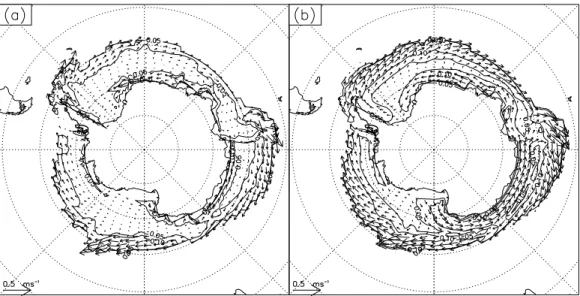
The dynamic sea ice rheology substantially affects the ice velocities (Fig. 3). In the SH speeds are faster with EVP although the broad scale pattern is similar. The fastest ice occurs around the coast of East Antarctica in response to the coastal easterlies, 5
and towards the edges of the pack in the zone of westerlies. EVP allows offshore advection of ice in the Ross Sea area, and produces a better-defined sea ice flow in the Weddell gyre, in better agreement with observations. In the NH (not shown) the effects within the Arctic basin are less, though ice speeds increase in the Bering strait and along the east coast of Greenland. The ice flow export through the Fram strait is 10
realistic, but the flow within the central arctic basin is not. This is largely due to the wind stress forcing: the model (as with the basic HadCM3) simulates too-high MSLP over the central arctic, and the Icelandic low is not deep enough. A lesser problem is the ocean circulation, which cannot be fully realistic due to the presence of a “polar island” introduced for numerical reasons, since the ocean model is on a regular grid. 15
For these reasons we focus more on the Antarctic simulation from the model. Figure 4 shows the affects of the rheology on the ice thickness in winter. In general the ice becomes thinner, as would be expected.
The degradation of some aspects of the simulation by adding EVP should not be too surprising as several of the thermodynamic parameterisations of HadCM3 had been 20
developed to work with the ocean drift sea ice. Hence, we next examine the effects of some physically based improvements to the thermodynamic parameterisations on the simulation.
5.2 The ice-ocean heat flux
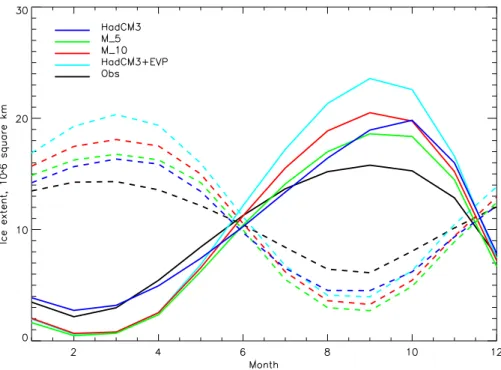
We present results of the M-scheme, in which the ice-ocean flux is made proportional to 25
the velocity shear between the ice and the ocean. This ocean-ice shear is highest near the edge of the pack, where the ice moves fastest, with values above 0.2 m/s; is above 0.1 m/s in much of the pack, declining to below 0.05 closer to the coast. Figure 5 shows
OSD
3, 777–803, 2006Implementation of elastic viscous plastic sea ice in
HadCM3 W. Connolley et al. Title Page Abstract Introduction Conclusions References Tables Figures J I J I Back Close
Full Screen / Esc
Printer-friendly Version Interactive Discussion
the difference in sea ice extent compared to the initial HadCM3+EVP run with values of C of 0.05 and 0.1 m/s. The new parameterisation makes a substantial contribution to reducing the difference between the observed and model ice extents in winter, although the summer extents are slightly worse in the Arctic.
We attempted to “tune” the model by adjusting the value of C within the physically 5
reasonable range. However, whilst changes do have an effect there is a trade-off be-tween summer and winter ice; decreasing C reduces the winter ice extent to more realistic values, but also decreases the summer ice to undesirably low values. We settled upon a value of 0.05 m/s.
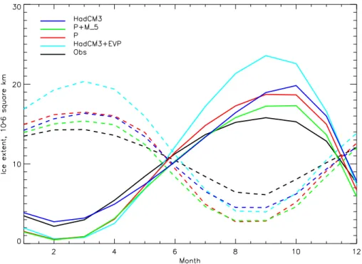
Further improvements are found with the P-scheme, in which the ice-ocean flux be-10
comes proportional to the ice area. Over marginal ice with a low fraction this is a near-neutral change; where the ice has a high fraction this potentially increases the ocean-ice flux and hence the ice melting. However the effect is not as large as might be expected because it is limited by the heat capacity of the ocean underneath the ice; this has been tested by increasing the diffusivity further, where it makes little differ-15
ence. The P-scheme has a major impact on the simulation (Fig. 6), particularly on the winter ice where the ice extent in both hemispheres is reduced back down to standard HadCM3 levels and much better agreement with observations. In summer, there is little effect in the SH whereas the extent reduces in the NH. Either P or M scheme results in significant changes to the sea ice extent; Fig. 6 also shows both schemes combined 20
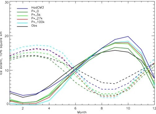
as HadCM3+P+M 10 which results is a further slight reduction in the ice extent. 5.3 Varying the ice-strength parameter P∗
Implementations of the Viscous-Plastic and EVP rheologies have tended to standardise around a value of 27.103 for P∗ (Hibler, 1979) but a range of values are used. In ocean-ice models forced by observed atmospheric fields, it is common to tune P∗ by 25
comparing against buoy data (or against observed ice thickness and other parameters; Miller at al., 2005); that method is not possible in a coupled ocean-atmosphere-seaice model and it may well be resolution-dependent. We investigate the influence of the
OSD
3, 777–803, 2006Implementation of elastic viscous plastic sea ice in
HadCM3 W. Connolley et al. Title Page Abstract Introduction Conclusions References Tables Figures J I J I Back Close
Full Screen / Esc
Printer-friendly Version Interactive Discussion
choice of P∗ on the simulation and find that higher values of P∗ tend to lead, in the SH, to more winter ice and less summer ice: see Fig. 7; as the ice becomes less compressible with higher P∗it is pushed further out. The sensitivity to P∗in this case is quite small – considerably smaller than the sensitivity to changes in the thermodynamic parameters. These runs are variations around the base state of HadCM3+M 10+P. 5
Greater sensitivity, with changes in the same sense (i.e. higher P∗ leading to more winter ice) is seen in runs using plain HadCM3+EVP as the base state – without the thermodynamic modifications detailed above.
In summer, in the SH, the (unreasonably high) value of P∗=105causes all the sum-mer ice to disappear, which is unrealisitic. Based on the SH results, one would choose 10
a value of P∗ as low as possible (even zero, which is free drift) for the best possible simulation of the ice extent. However, this is not compatible with observations and the-ory. Also, in the NH, a P∗ of zero degrades the summer simulation. Based on these results and the range of values in the literature, we choose a value of 5.103for P∗.
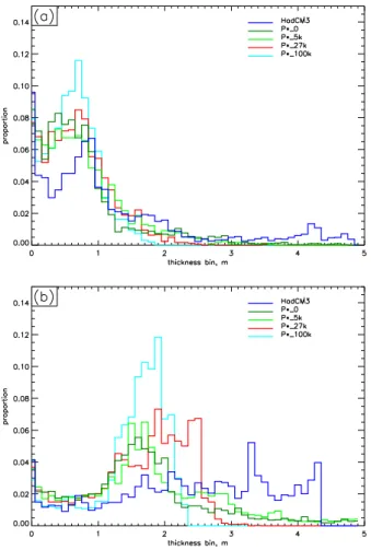
Figure 8 shows histograms of the seaice thickness for various values of P∗. As 15
expected, higher values of P∗make the ice less compressible and hence more ice is of lower thickness. This is more noticeable in the NH, where rheology is more important. For P∗=0 in the NH there is a long “tail” of ice of very high thickness, since the ice has no strength. By comparison, the HadCM3 thickness histogram is very different, again reflecting the lack of a proper rheology in that model.
20
6 Optimised EVP run
Combining all the changes, we come to a “best” EVP run as follows:
– McPhee ocean to ice heat flux with C=0.05 m s−1, scaled by the ice concentration and with K=2.5.10−4m2s−1
– P∗=5.103
25
OSD
3, 777–803, 2006Implementation of elastic viscous plastic sea ice in
HadCM3 W. Connolley et al. Title Page Abstract Introduction Conclusions References Tables Figures J I J I Back Close
Full Screen / Esc
Printer-friendly Version Interactive Discussion
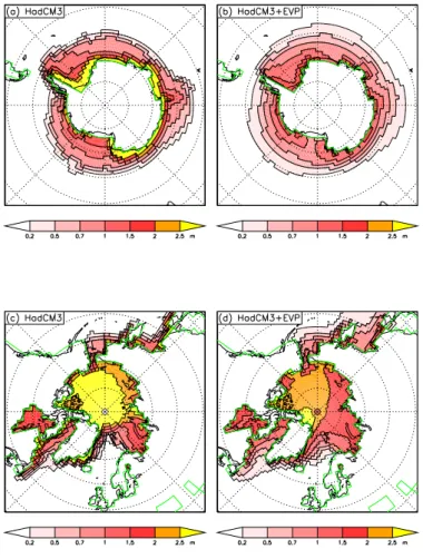
Maps of the maximum ice extent for this run are shown in Fig. 9, and the remainder of the paper shows results from this optimised run. Of the changes, adding the improved (EVP) dynamics has a substantial effect on the sea ice simulation. Having done that, further tuning of the dynamics (via plausible values for P∗) has comparatively little ef-fect, as shown by Fig. 7. Tuning the thermodynamics has rather larger effects. This 5
run improves over HadCM3 by a better (reduced) winter sea ice extent in both hemi-spheres, but suffers from too little ice in the summer; the seasonal cycle remains too large. The successor to HadCM3, HadGEM1 (Hadley Centre Global Environmental Model version 1), uses much the same EVP scheme as here for the dynamics but introduces ice thickness categories for the thermodynamics and ridging and this has 10
further large effects (McLaren et al., 2006). The spatial distribution of ice thickness in HadGEM1 is much improved in both hemispheres
7 Stress balance in the model
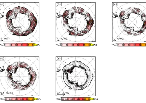
We now consider the balance of forces within the sea ice. Figure 10 shows a snapshot of this for a typical day in the southern hemisphere. As noted above in Sect. 5.1, there 15
are deficiencies in the northern hemisphere simulation (largely unrelated to the sea ice model itself) so we do not show the NH. The main terms in the balance for the Antarctic are the wind and water stresses; the Coriolis force is weaker, and the internal stresses in general weaker still. Much of the Antarctic ice is close to free-drift balance; exceptions to this are in the Weddell sea and around the coastlines. The existence 20
of the free-drift balance is not surprising, since the ice is generally unconstrained by land boundaries and often in divergent flow. However, the internal stress component of the force balance is still important in influencing the ice behaviour on the large scale: as Fig. 7 shows, the total ice extent is sensitive to changes in the internal ice strength parameter, P∗. In the Arctic, the dominant balance is still between wind and water 25
stresses, but the internal force is larger and significant across the basin. Because of atmospheric circulation errors (not shown) the maximum ice thickness is in the central
OSD
3, 777–803, 2006Implementation of elastic viscous plastic sea ice in
HadCM3 W. Connolley et al. Title Page Abstract Introduction Conclusions References Tables Figures J I J I Back Close
Full Screen / Esc
Printer-friendly Version Interactive Discussion
Arctic rather than against the Canadian archipelego as it should be; this in turn means that the largest internal ice stresses are not in the correct place.
8 Effects on variability
Holland and Raphael (2006) note that the variability of sea ice around Antarctica in climate models is significantly larger than in the observations. For September in the 5
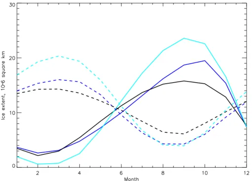
Antarctic, over the period 1979–2002, the standard deviation (SD, in 106km2) of ice extent from the Bootstrap algorithm is 0.32. HadCM3 gives a substantially larger value, 1.13. EVP has a variability that matches the observations. Looking at the variability throughout the year, the picture (see Fig. 11) becomes more interesting.
EVP correctly reproduces the form of the curve, with maxima in January and April 10
and minima in February and August. EVP is somewhat too variable, especially at times of larger ice extent. By contrast, HadCM3 has completely the wrong pattern of variability throughout the year, and shows far too much variability, especially in winter and spring.
A different way of examining the variability is to look at the standard deviation of 15
the ice cover, point-wise. For September, this has total values (106km2) of 2.5, 3.2, 2.3 for Bootstrap, HadCM3 and EVP respectively. These numbers are larger than the SD of the area-total ice extent, because they include variations in the ice pattern (if the variability were purely that the ice anomalies rotated around the continent without changing overall area, for example, then the SD of total ice extent would be zero, but 20
the total of the ice SD would be non-zero). These values imply that HadCM3 has more variability in spatial location of the anomalies than the observations or EVP. This is confirmed by EOF analysis (not shown): the first EOF of the observations, and EVP, have their variance largely confined to the sector (145◦W, 0◦E) whereas HadCM3 has large variance between (0◦E, 135◦E).
25
For the Arctic (not shown) variability is around 0.4 106km2 year-round; HadCM3 reproduces this both with and without EVP. This may be because of the different
OSD
3, 777–803, 2006Implementation of elastic viscous plastic sea ice in
HadCM3 W. Connolley et al. Title Page Abstract Introduction Conclusions References Tables Figures J I J I Back Close
Full Screen / Esc
Printer-friendly Version Interactive Discussion
namics dominating in the land-locked Arctic basin.
9 Other sources of error in the sea ice model
In a coupled model, even a perfect sea ice model would not produce a perfect sim-ulation due to deficiencies in other model components. We are not in a position to closely examine deficiencies in the ocean model, but there exist large Mean Sea Level 5
Pressure (MSLP) errors in HadCM3 (Fig. 12) which imply errors in the wind stress forc-ing of the sea ice model (as found by Bitz, 2002). The largest error is a northwards wind stress at around 90◦E, which is consistent with the excess ice at this longitude within this model. The southwards error in the Amundsen-Bellingshausen sea is com-patible with the deficit of sea ice there. The MSLP errors appear to be related to the 10
tropical sea surface temperature errors in HadCM3, in particular those near Indone-sia (Lachlan-Cope, Connolley and Turner, submitted) and not strongly related to local conditions. Hence they cannot readily be cured, and the sea ice simulation must be evaluated in the context of these errors.
10 Conclusions
15
This paper has documented the implementation of the Elastic Viscous Plastic sea ice rheology within the coupled ocean-sea-ice-atmosphere GCM HadCM3. We show that this more physically based rheology nonetheless initially degrades the sea ice simula-tion, but that a number of the thermodynamic parametrisations relating to the ocean-ice heat flux within the default HadCM3 sea ice scheme can also be improved, and follow-20
ing this the overall sea ice simulation is generally better than HadCM3. Also, since it is now more physically based, we have more confidence in the model both for hindcasts and forecasts of climate change. An initial finding is that the interannual variability is in much better agreement with the observations that the original HadCM3 model. Further
OSD
3, 777–803, 2006Implementation of elastic viscous plastic sea ice in
HadCM3 W. Connolley et al. Title Page Abstract Introduction Conclusions References Tables Figures J I J I Back Close
Full Screen / Esc
Printer-friendly Version Interactive Discussion
work on the sea ice model will take place within the framework of the HadGEM model (McLaren et al., 2006), centering on the issues of multi-category sea ice and further improvements to the thermodynamics.
Acknowledgements. We are grateful to D. Cresswell, who did the programming of the initial implementation of EVP into HadCM3.
5
References
Bitz, C. M., Fyfe, J. C., and Flato, G. M.: Sea Ice Response To Wind Forcing From AMIP Models, J. Climate, 15, 522–536, 2002.
Comiso, J.: Bootstrap sea ice concentrations for NIMBUS-7 SMMR and DMSP SSM/I, June to September 2001, Boulder, CO, USA: National Snow and Ice Data Center, Digital media,
10
http://www.nsidc.org/data/nsidc-0079.html, 1999, updated 2003.
Comiso, J. C. and Steffen, K.: Studies Of Antarctic Sea Ice Concentrations From Satellite Data And Their Applications, J. Geophys. Res., 106, 31 361–31 385, 2002.
Connolley, W. M.: Sea ice concentrations in the Weddell Sea: A comparison of SSM/I, ULS, and GCM data, Geophys. Res. Lett., 32, 7, art. no. L07501 APR 2, 2005.
15
Holland, M. M. and Raphael, M. N.: Twentieth century simulation of the southern hemisphere climate in coupled models. Part II: sea ice conditions and variability, Clim. Dyn., 26, 229–245, doi:10.1007/s00382-005-0087-3, 2006.
Hunke, E. C. and Dukowicz, J. K.: An Elastic-Viscous-Plastic Model For Sea Ice Dynamics, J. Phys. Oceangr., 27, 1849–1867, 1997.
20
Gordon, C., Cooper, C., Senior, C. A., Banks, H., Gregory, J. M., Johns, T. C., Mitchell, J. F. B., and Wood, R. A.: The Simulation Of Sst, Sea Ice Extents And Ocean Heat Transports In A Version Of The Hadley Centre Coupled Model Without Flux Adjustments, Clim. Dyn., 16, 147–168, 2000.
McLaren, A. J., Banks, H. T., Durman, C. F., Gregory, J. M., Johns, T. C., Keen, A. B., Ridley,
25
J. K., Roberts, M. J., Lipscomb, W. H., Connolley, W. M., and Laxon, S. W.: Evaluation of the Sea Ice Simulation in a new Coupled Atmosphere-Ocean Climate Model (HadGEM1), J. Geophys. Res. (Oceans), in press, 2006.
OSD
3, 777–803, 2006Implementation of elastic viscous plastic sea ice in
HadCM3 W. Connolley et al. Title Page Abstract Introduction Conclusions References Tables Figures J I J I Back Close
Full Screen / Esc
Printer-friendly Version Interactive Discussion
McPhee, M. G.: Turbulent heat flux in the upper ocean under sea ice, J. Geophys. Res., 97, C4, 5365–5379, 1992.
Mcphee, M. G., Kottmeier, C., and Morison, J. H.: Ocean Heat Flux In The Central Weddell Sea During Winter, J. Phys. Oceangr., 29, 1166–1179, 1999.
Miller, P. A., Laxon, S. W., and Feltham, D. L.: Improving The Spatial Distribution Of Modeled
5
Arctic Sea Ice Thickness, Geophys. Res. Lett., 32, Art. No. L18503, 2005.
Pope, V. D., Gallani, M. L., Rowntree, P. R., and Stratton, R. A.: The impact of new physical parametrisations in the Hadley Centre climate model: HadAM3, Clim. Dyn., 16, 123–146, 2000.
Semtner, A. J.: A model for the thermodynamic growth of sea ice in numerical investigations of
10
climate, J. Phys. Oceanogr., 6, 379–389, 1976.
Turner, J., Connolley, W. M., Cresswell, D., and Harangozo, S. A.: The simulation of Antarctic sea ice in the Hadley Centre Climate Model (HadCM3), Ann. Glaciol., 33, 585–591, 2001. Turner, J., Connolley, W. M., Lachlan-Cope, T. A., and Marshall, G. J.: The performance of
the Hadley Centre Climate Model (HadCM3) in high southern latitudes, Int. J. Climatol., 26,
15
91–112, 2006.
OSD
3, 777–803, 2006Implementation of elastic viscous plastic sea ice in
HadCM3 W. Connolley et al. Title Page Abstract Introduction Conclusions References Tables Figures J I J I Back Close
Full Screen / Esc
Printer-friendly Version Interactive Discussion
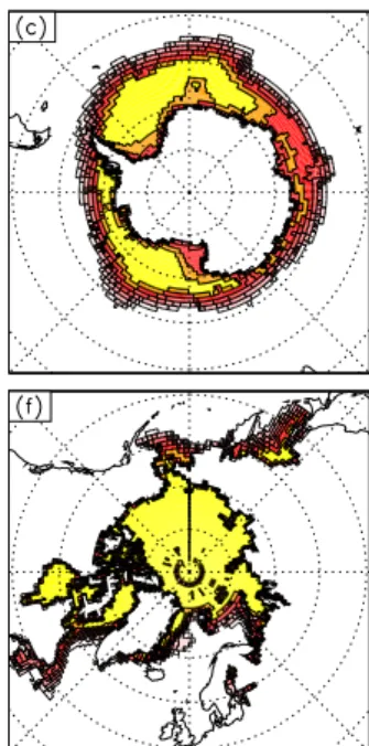
Fig. 1. Sea ice at maximum extent from HadCM3, initial HadCM3+EVP and observations (a– c): September in the SH; (d–f): March in the NH. (a), (d): HadCM3; (b), (e): HadCM3+EVP;
(c), (f): Observations.
OSD
3, 777–803, 2006Implementation of elastic viscous plastic sea ice in
HadCM3 W. Connolley et al. Title Page Abstract Introduction Conclusions References Tables Figures J I J I Back Close
Full Screen / Esc
Printer-friendly Version Interactive Discussion
Fig. 2. Annual cycle of ice extent from HadCM3 (blue), HadCM3+EVP (light blue) and
obser-vations (black). Southern hemisphere, solid lines. Northern hemisphere, dashed lines.
OSD
3, 777–803, 2006Implementation of elastic viscous plastic sea ice in
HadCM3 W. Connolley et al. Title Page Abstract Introduction Conclusions References Tables Figures J I J I Back Close
Full Screen / Esc
Printer-friendly Version Interactive Discussion
Fig. 3. Sea ice velocity in September from (a) HadCM3 and (b) HadCM3+EVP; contour interval
0.05 ms−1.
OSD
3, 777–803, 2006Implementation of elastic viscous plastic sea ice in
HadCM3 W. Connolley et al. Title Page Abstract Introduction Conclusions References Tables Figures J I J I Back Close
Full Screen / Esc
Printer-friendly Version Interactive Discussion
Fig. 4. Ice thickness for (a) HadCM3 (b) HadCM3+EVP for the southern hemisphere. (c), (d)
the same, for the northern hemisphere.
OSD
3, 777–803, 2006Implementation of elastic viscous plastic sea ice in
HadCM3 W. Connolley et al. Title Page Abstract Introduction Conclusions References Tables Figures J I J I Back Close
Full Screen / Esc
Printer-friendly Version Interactive Discussion
Fig. 5. Response of ice extent to variation in the ice-ocean heat flux. Black, observations; Blue,
HadCM3; light blue, HadCM3+EVP. Red, HadCM3+M-10; Green, HadCM3+M 5. Solid lines: SH; dashed lines: NH.
OSD
3, 777–803, 2006Implementation of elastic viscous plastic sea ice in
HadCM3 W. Connolley et al. Title Page Abstract Introduction Conclusions References Tables Figures J I J I Back Close
Full Screen / Esc
Printer-friendly Version Interactive Discussion
Fig. 6. Response of ice extent to variation in the ice-ocean heat flux P scheme. Black,
observa-tions; Blue, HadCM3; light blue, HadCM3+EVP. Red, HadCM3+P; Green, HadCM3+P+M 5. Solid lines: SH; dashed lines: NH.
OSD
3, 777–803, 2006Implementation of elastic viscous plastic sea ice in
HadCM3 W. Connolley et al. Title Page Abstract Introduction Conclusions References Tables Figures J I J I Back Close
Full Screen / Esc
Printer-friendly Version Interactive Discussion
Fig. 7. Response of ice extent to variation in P∗. Black, observations; Blue, HadCM3. Dark green, light green red and light blue are, respectively, P∗=0, 5, 27 and 100.103 in HadCM3+P+M 10+P∗
. Solid lines: SH; dashed lines: NH.
OSD
3, 777–803, 2006Implementation of elastic viscous plastic sea ice in
HadCM3 W. Connolley et al. Title Page Abstract Introduction Conclusions References Tables Figures J I J I Back Close
Full Screen / Esc
Printer-friendly Version Interactive Discussion
Fig. 8. Histogram of sea ice thickness in September (Antarctic, top) and March (Arctic, bottom).
Blue, HadCM3. Dark green, light green red and light blue are, respectively, P∗=0, 5, 27 and 100.103in HadCM3+P+M 10+P∗.
OSD
3, 777–803, 2006Implementation of elastic viscous plastic sea ice in
HadCM3 W. Connolley et al. Title Page Abstract Introduction Conclusions References Tables Figures J I J I Back Close
Full Screen / Esc
Printer-friendly Version Interactive Discussion
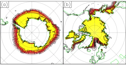
Fig. 9. Seaice extent at winter maximum in the optimised run HadCM3+P+M 5+P∗5k, (a)
southern hemisphere in September and(b) northern hemisphere in March.
OSD
3, 777–803, 2006Implementation of elastic viscous plastic sea ice in
HadCM3 W. Connolley et al. Title Page Abstract Introduction Conclusions References Tables Figures J I J I Back Close
Full Screen / Esc
Printer-friendly Version Interactive Discussion
Fig. 10. Ice velocity and force terms in the momentum equation for a typical winter day,
2003/09/22. (a): ice velocity. (b): wind stress; (c): ice-ocean stress; (d): coriolis force; (e)
internal stress. Note the changes of scale between the plots.
OSD
3, 777–803, 2006Implementation of elastic viscous plastic sea ice in
HadCM3 W. Connolley et al. Title Page Abstract Introduction Conclusions References Tables Figures J I J I Back Close
Full Screen / Esc
Printer-friendly Version Interactive Discussion
Fig. 11. Interannual standard deviation of total ice extent in the southern hemisphere by month.
Black: observations; blue: HadCM3; red: EVP.
OSD
3, 777–803, 2006Implementation of elastic viscous plastic sea ice in
HadCM3 W. Connolley et al. Title Page Abstract Introduction Conclusions References Tables Figures J I J I Back Close
Full Screen / Esc
Printer-friendly Version Interactive Discussion
Fig. 12. Geopotential height difference at 500 hPa between HadCM3 and ERA, together with
implied geostrophic wind anomalies.