HAL Id: hal-00296217
https://hal.archives-ouvertes.fr/hal-00296217
Submitted on 8 May 2007
HAL is a multi-disciplinary open access
archive for the deposit and dissemination of
sci-entific research documents, whether they are
pub-lished or not. The documents may come from
teaching and research institutions in France or
abroad, or from public or private research centers.
L’archive ouverte pluridisciplinaire HAL, est
destinée au dépôt et à la diffusion de documents
scientifiques de niveau recherche, publiés ou non,
émanant des établissements d’enseignement et de
recherche français ou étrangers, des laboratoires
publics ou privés.
aerosol modules
D. K. Weisenstein, J. E. Penner, M. Herzog, X. Liu
To cite this version:
D. K. Weisenstein, J. E. Penner, M. Herzog, X. Liu. Global 2-D intercomparison of sectional and
modal aerosol modules. Atmospheric Chemistry and Physics, European Geosciences Union, 2007, 7
(9), pp.2339-2355. �hal-00296217�
www.atmos-chem-phys.net/7/2339/2007/ © Author(s) 2007. This work is licensed under a Creative Commons License.
Chemistry
and Physics
Global 2-D intercomparison of sectional and modal aerosol modules
D. K. Weisenstein1, J. E. Penner2, M. Herzog2,*, and X. Liu2,**
1Atmospheric and Environmental Research, Inc., Lexington, MA, USA
1Department of Atmospheric, Oceanic, and Space Sciences, University of Michigan, Ann Arbor, MI, USA *now at: NOAA Geophysical Fluid Dynamics Laborator, Princeton, NJ, USA
**now at: Pacific Northwest National Laboratory, Richland, WA, USA
Received: 30 October 2006 – Published in Atmos. Chem. Phys. Discuss.: 7 December 2006 Revised: 23 March 2007 – Accepted: 21 April 2007 – Published: 8 May 2007
Abstract. We present an intercomparison of several aerosol
modules, sectional and modal, in a global 2-D model in or-der to differentiate their behavior for tropospheric and strato-spheric applications. We model only binary sulfuric acid-water aerosols in this study. Three versions of the sectional model and three versions of the modal model are used to test the sensitivity of background aerosol mass and size distribu-tion to the number of bins or modes and to the prescribed width of the largest mode. We find modest sensitivity to the number of bins (40 vs. 150) used in the sectional model. Aerosol mass is found to be reduced in a modal model if care is not taken in selecting the width of the largest lognormal mode, reflecting differences in sedimentation in the middle stratosphere. The size distributions calculated by the sec-tional model can be better matched by a modal model with four modes rather than three modes in most but not all sit-uations. A simulation of aerosol decay following the 1991 eruption of Mt. Pinatubo shows that the representation of the size distribution can have a signficant impact on model-calculated aerosol decay rates in the stratosphere. Between 1991 and 1995, aerosol extinction and surface area density calculated by two versions of the modal model adequately match results from the sectional model. Calculated effective radius for the same time period shows more intermodel vari-ability, with a 20-bin sectional model performing much better than any of the modal models.
1 Introduction
Aerosols are important to the radiative balance and chem-istry of the atmosphere, and can modify cloud properties. In the stratosphere, aerosol particles provide surfaces for het-erogeneous chemistry, modifying the ratio of active NOx, Correspondence to: D. K. Weisenstein
HOx, ClOx, and BrOx radicals to reservoir species (Fahey
et al., 1993; Wennberg et al., 1994) and thus modifing ozone concentrations following volcanic eruptions (Hofmann and Solomon, 1989). In the troposphere, aerosol particles can act as cloud condensation nuclei, influencing cloud droplet number density and size (Penner et al., 2001), and thus cloud albedo. They also have direct radiative effects (Haywood and Ramaswamy, 1998) and can modify atmospheric circulation (Labitzke and McCormick, 1992; McCormick, et al., 1995) and temperature (Hansen et al., 2002).
This study was motivated by the requirements of the Global Modeling Initiative (GMI) 3-D chemical-transport model (Rotman et al., 200). The GMI model was created to be modular and permit intercomparisons between differ-ent process modules as a way of studying model sensitivity. It uses a variety of wind fields, from both assimilation sys-tems and GCM simulations (Douglass et al., 1999; Strahan and Douglass, 2004). It can also use a variety of chemi-cal schemes and parameterizations (Considine et al., 2000; Douglass et al., 2004). Sulfur chemistry and aerosol micro-physics from the University of Michigan 3-mode model have been added to the tropospheric version of GMI (Liu et al., 2005). Eventually the GMI will operate with aerosol micro-physics in a version which will span both troposphere and stratosphere, and can run with either a sectional or modal aerosol representation. This study tests and contrasts these two representations of aerosol size distribution in a 2-D model of the troposphere and stratosphere for both accuracy and computational efficiency.
Tropospheric aerosol models must deal with many types of aerosols, including sulfate, dust, sea salt, organics, and black carbon. Because of the computational requirements of 3-D tropospheric models, the prediction of aerosol mass was often considered adequate and fixed size distributions were assumed to evaluate radiative effects (Penner et al., 2001, 2002). More recent models have added the predic-tion of number density and size distribupredic-tion using efficient
methods such as modal representations (Wilson et al., 2001; Liu et al., 2005; Stier et al., 2005) or the method of moments (Wright et al., 2001). Regional tropospheric models have employed more detailed sectional representations (Jacobson, 2001; Zhang et al., 2004) to predict particle size distributions without imposing an a priori shape on the distribution.
Stratospheric aerosol models generally differ from tropo-spheric aerosol models because resolving the size distribu-tion of aerosol particles becomes more important at altitudes above the tropopause. In the troposphere, only particles larger than ∼1 µm settle appreciably, whereas the thinner air in the stratosphere causes sedimentation rates to be a strong function of both particle radius and air density. Even parti-cles of 0.01 µm radius have significant sedimentation rates at 30 km. Resolving the size distribution of aerosol parti-cles is crucial to predicting the correct sedimentation rate and therefore the lifetime and vertical distribution of par-ticles in the stratosphere. Thus stratospheric models have generally used the sectional approach to resolve size distri-butions (Weisenstein et al., 1997; Timmreck, 2001; Pitari et al., 2002). Yet the sectional approach leads to numerical dif-fusion in size space, which may be excessive for a coarse resolution sectional model. The computational expense of a sectional model is mitigated for stratospheric studies because non-sulfate particles are not important in much of the strato-sphere and therefore are generally omitted.
Many of the sulfur source gases are short-lived and have localized emissions, such as industrial sources. Rapid trans-port in convective cells is believed to play an imtrans-portant role in moving sulfur source gases from the boundary layer to the upper troposphere, where they may interact with clouds. Transport by diabatic ascent, cloud outflow, and horizontal motion moves sulfur from the troposphere into the strato-sphere. Thus detailed modeling of tropospheric transport, cloud interactions, and microphysics is important to predict-ing the sulfur enterpredict-ing the stratosphere. For these reasons, we believe it important to model tropospheric and stratospheric aerosols together in a 3-D model like the GMI.
The University of Michigan aerosol module, referred to as UMaer, is described in Herzog et al. (2004). That paper applied the aerosol module within a zero-dimensional box model and compared results with the Atmospheric and Envi-ronmental Research (AER) sectional model using 40 or 150 bins. In that intercomparison, both models were thoroughly tested until the only remaining differences were due to the representation of the size distribution; differences in micro-physical parameterizations were removed. Here that inter-comparison is extended to two dimensions so that the impact of the different representations of size distribution will be seen in the model transport and sedimentation as well. The 2-D study is performed prior to implementation of aerosol microphysics in the stratosphere-troposphere GMI for effi-ciency. While details of tropospheric chemistry and transport are missing here, the stratospheric results in 2-D should not differ appreciably from stratospheric results in 3-D. Thus we
focus most of our intercomparisons and comparisons with observations on the stratosphere. We have performed simu-lations of sulfate aerosol under background nonvolcanic con-ditions and a time dependent simulation from 1991 to 1999 including the Mt. Pinatubo eruption.
This paper presents descriptions of the 2-D model frame-work used as the intercomparison tool and the two aerosol modules in Sect. 2. In Sect. 3 we describe the intercom-parison approach and model versions tested (three sectional, three modal). Section 4 provides results of a background atmosphere calculation in the troposphere and stratosphere, showing how differences in aerosol representation affect model results. Section 5 shows results of a volcanic simu-lation and the differences in aerosol removal rates with the different approaches. A summary and discussion is provided in Sect. 6.
2 Model descriptions
The AER 2-D model is used as the framework for this inter-comparison, with transport, sulfur chemistry, and aerosol mi-crophysics performed for the global domain from the surface to 60 km. Grid resolution is 9.5◦ in latitude and 1.2 km in the vertical. Transport is effected by the residual circulation and by horizontal and vertical diffusion. We use transport parameters from Fleming et al. (1999) which are calculated from observed ozone, water vapor, zonal wind, and tempera-ture for climatological conditions. Wave driving is provided by forcing from six planetary waves and the effects of gravity wave breaking. Diabatic heating rates are computed follow-ing Rosenfield et al. (1994), with tropospheric latent heatfollow-ing from Newell et al. (1974). The calculation of horizontal dif-fusion coefficients follows Randel and Garcia (1994).
Since we are modeling sulfate aerosols for this intercom-parison, we model only sulfur chemistry and use necessary radical concentrations from other model simulations. Sulfur source gases include DMS, H2S, CS2, OCS, and SO2.
Sur-face fluxes are 25 MT sulfur per year from DMS, 1 MT sulfur from CS2, 8.7 MT sulfur from H2S, and 78 MT sulfur from
SO2. In addition, we assume a surface mixing ratio for OCS
of 500 pptv which provides a stratospheric source of sulfur. Photolysis and reactions with OH, O, O3, and NO3convert
sulfur source gases to sulfuric acid. Concentrations of these reactants are taken from a present-day simulation with the AER 2-D chemical-transport model and vary seasonally. De-tails of the chemical scheme can be found in Weisenstein et al. (1997). Reaction rates are taken from the JPL 2002 com-pendium (Sander et al., 2003). Homogeneous nucleation of sulfuric acid vapor occurs chiefly in the tropical upper tropo-sphere due to low temperatures and high relative humidity. Subsequently, condensation increases the size of particles, while coagulation limits their number density. Evaporation occurs in the 30–40 km altitude region, yielding H2SO4
The University of Michigan aerosol module (UMaer) is capable of treating the nucleation and growth of sulfuric acid-water aerosols, as well as their coagulation with nonsulfate particles (Herzog et al., 2004). Aerosol size distributions, defined by N (r), particle number concentration at radius r, are treated by predicting two moments (mass and number) of the two or more lognormal distributions
dN (r) dr = N0 √ 2π rgln σg exp(−1 2 ln2(r/rg) ln2σg ) (1)
each of which is defined by a mode radius rg and a distribu-tion width σg. The distribution width is specified. As mass is added to each mode and the particles grow, a merging pro-cess shifts mass from mode to mode, keeping the mode radii within defined bounds. The module performs dynamic time stepping without operator splitting such that all aerosol pro-cesses interact with each other during each time step. It can be applied to both tropospheric and stratospheric conditions, but to date has been used only in the troposphere and lower-most stratosphere.
The AER 2-D sulfate aerosol model was described in Weisenstein et al. (1997, 1998). The aerosol module uses a sectional representation of the particle size distribution and can represent any arbitrary distribution shape. Particle num-ber density in 40 bins between 0.4 nm and 3.2 µm by volume doubling is predicted, though the bin number, smallest bin radius, and volume ratio between bins are adjustable parame-ters. The model is intended for stratospheric applications and includes only sulfuric acid-water particles. Aerosol compo-sition, or weight fractions of sulfate and water, is adjusted continuously based on ambient temperature and relative hu-midity according to Tabazadeh et al. (1997). Particle sizes are based on both sulfate and water fractions, so that parti-cles grow or shrink when either temperature or water vapor concentration changes in a grid box. The microphysical so-lution uses operator splitting with a time step of one hour for transport, chemistry, and microphysics, but 20 substeps for the condensation and nucleation processes to prevent one process from dominating the gas-to-particle exchange rate.
Our goal in this intercomparison, and our previous box model intercomparison (Herzog et al., 2004) was to com-pare microphysical modules which are identical except in the way that the size distribution is represented. To that end, we have compared each aerosol process carefully and ensured that initial tendencies are identical. We use the Vehkamaeki et al. (2002) nucleation parameterization, which is in agree-ment with more detailed calculations of hydrated clusters for temperatures greater than 190 K. The parameterization cal-culates the radius, composition, and production rate of new particles. The UMaer module adds the new particle number and mass to the smallest aerosol mode, exactly preserving the calculated number density. The AER module requires that the nucleated mass be added to a single bin with a fixed radius, so particle number is adjusted to preserve the calcu-lated nucleation mass.
The condensation and evaporation process is treated as de-scribed in Herzog et al. (2004). The condensational growth or evaporation in each bin or mode depends of the difference in the gas phase H2SO4 concentration, Ngas, and the
equi-librium concentration of H2SO4 above the particle surface,
Nequgas, and is described by
∂
∂tNgas= −4πβD(Ngas− N
equ
gas)rpNp (2) where β is a term correcting for noncontinuum effects and imperfect surface accomodation, D is the diffusion coeffi-cient for H2SO4molecules in air, and Npis the number den-sity of particles in the bin or mode. For the sectional model, rp is the bin radius. For the modal model, the appropriate radius rpdepends on the volume mean wet radius, rvol, and
the width of the lognormal distribution, σg,
rp= rvolexp(− ln2σg). (3)
Wet radius is calculated using the Tabazadeh et al. (1997) parameterization for aerosol composition. The Kelvin effect is included in the calculation of Nequgas and depends upon
par-ticle radius. The modal model uses volume mean radius in this calculation, and for calculation of the Knudsen number when calculating β. Condensation doesn’t change the num-ber of particles, only the mass in each mode for the modal model. In the sectional model, condensational growth shifts particles to larger bin sizes. Evaporation does the opposite, shifting particles to smaller sizes, but net number density is only reduced for evaporation from the smallest bin size or mode.
The coagulation process reduces number concentration and shifts aerosol mass into larger particles. A coagulation kernel defines the collision probability of two paticles of dif-ferent radii, and depends on the radius of each particle and the particle diffusion coefficients. The modal model uses volume mean wet radius for this calculation. In the sec-tional model, when two particles of radii ri and rj collide, where ri<rj, a particle is removed from bin i and a new particle with size intermediate to bin j and bin j +1 is cre-ated. We apportion the particle mass between the two bins but this process results in numerical diffusion in size space. If the ratio of adjacent bin volumes is 2.0, then coagulation of two particles in bin j results in a particles of exactly ra-dius rj +1. In the modal model, coagulation within a mode results in a reduction in number in that mode. Coagulation between modes results in a reduction in mass and number of the smaller mode and an increase of mass in the larger mode. The sedimentation process affects the vertical distribution of aerosol sulfate, particularly in the middle stratosphere, and reduces the residence time of particles. The gravitational set-tling velocity of a particle with radius rpis given by
νgrav= 2 9 g ηair rp2ρp h 1+Kn[1.257+0.4 exp(−1.1Kn−1]i (4)
Table 1. Model versions used in 2-D intercomparison study.
Module Label Bin ratios Time step Run time
by volume rel. to AER40
AER 150 bins AER150 Vrat=1.2 15 min 20
AER 40 bins AER40 Vrat=2.0 1 h 1.0
AER 20 bins AER20 Vrat=4.0 1 h 0.25
Module Label Distribution Merge radii Run time
width σg rel. to AER40
UMaer 3 modes UMaer-3mA 1.2/1.514/1.77623 0.005/0.05 0.7 UMaer-3mB 1.2/1.514/1.6 0.005/0.05 0.7 UMaer 4 modes UMaer-4m 1.3/1.6/1.6/1.45 0.001/0.01/0.1 1.1
with
Kn = λrair p
(5)
according to Stokes law with the Cunningham slip correc-tion factor (Seinfeld and Pandis, 1997). Here λairis the mean
free path of air and ηairis the viscosity of air. The sectional
model applies the above settling velocity for each bin. The modal model applies one settling velocity per mode, replac-ing rpwith an effective radius appropriate for sedimentation of aerosol number
rpnum= rvolexp(−0.5 ln2σg) (6)
or for sedimentation of aerosol mass
rpmass= rvolexp(2.5 ln2σg). (7)
Since settling velocity is quite sensitive to particle radius for submicron particles at altitudes above about 25 km, we ex-pect that the difference in a modal and a sectional model may be pronounced above 25 km.
The box model intercomparison between these two aerosol modules (Herzog et al., 2004) showed that the modal model was capable of predicting both aerosol number concentration and surface area to within a factor of 1.2 (4 modes) or 1.3 (2 modes) on average as compared to the sectional model. Pre-diction of accumulation mode particle number concentration was not as accurate but still generally within a factor of 2.1. This intercomparison is performed within a 2-D model in or-der to compare differences due to transport and sedimenta-tion over seasonal and decadal time scales. In the secsedimenta-tional model, transport occurs independently for each size bin. In the modal model, transport modifies the number and mass for each mode. Sedimentation in the modal model is a function of the assumed distribution width, since the larger tail of the distribution is much more sensitive to settling, yet the entire modal distribution is given the same settling velocity. Sedi-mentation not only removes particles from a given grid box,
it also moves particles from higher to lower altitudes, affect-ing local size distributions and vertical mass profiles. We ex-pect sedimentation to contribute to much of the difference be-tween model-calculated aerosol distributions, and therefore we perform some calculations with and without sedimenta-tion.
3 Intercomparison approach
Our intercomparison approach is to apply the different aerosol modules within the same 2-D chemical-transport model. Thus transport and chemistry are treated identically insofar as possible. We use the AER sectional model with 20, 40 bins, or 150 bins. The 40-bin version is our standard treat-ment. The 150-bin version is computationally expensive, but reduces the numerical diffusion inherent in a sectional model. We treat this version as the most accurate model numeri-cally, thus allowing us to analyze deficiencies in the AER 40-bin model. A low-resolution 20-bin model is also used. The UMaer modal model is run with three modes and with four modes. We present two 3-mode versions differing in the width, σg, of the largest mode. For each modal model, we specify the distribution width and size limits of the modes. The model versions and their defining parameters are listed in Table 1. Also shown in Table 1 are the time steps used in the sectional models and the runtime of each model rel-ative to the AER40 version. Each model is run to steady-state for a background atmosphere case without volcanic in-fluence. The final state is independent of the initial condition. Most of these cases are also run in time-dependent mode for a Pinatubo-like injection of volcanic SO2in the tropical
strato-sphere, so that we can compare the volcanic aerosol decay rates over an eight year period. These calculations are ini-tialized with the steady-state background condition for the respective model.
Each model version covers the diameter range from sub-nanometer to about 3 µm. In the sectional model, the bin spacing is described by the parameter Vratwhich is the ratio
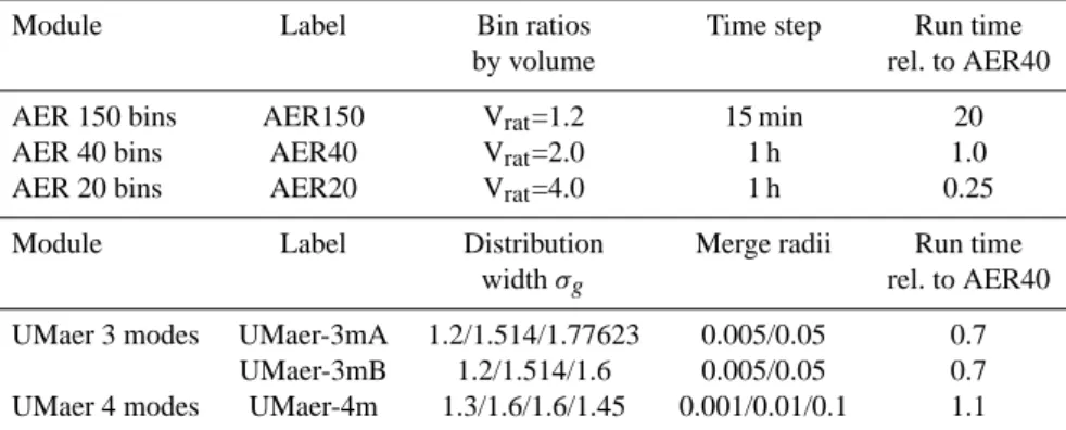
(a) (b)
( ) (d)
Fig. 1. Model calculated aerosol parameters from the AER 2-D model using the 150-bin sectional aerosol module AER150. Shown are
annual average (a) mass density in µg/m3, (b) surface area density in µm2/cm3, (c) effective radius in µm, and (d) number density of particles with radius greater than 0.05 µm in cm−3.
of particle volumes between adjacent bins. Typical strato-spheric aerosol sectional models (see Bekki and Pyle, 1992; Mills et al., 1999; Timmreck, 2001) employ Vrat values of
2.0, as does our 40-bin model. Our 150-bin model uses a Vrat
of 1.2 to cover the same radius space. Numerical stability demands smaller time steps as the number of bins increases. We use a 15 min time step for the 150-bin model and a one hour time step for the 40-bin and 20-bin models, in each case applying 20 substeps for condensation and nucleation.
The modal model specifies the width of each mode, σg. In addition, merge radii are required which specify when aerosol mass is shifted to the next larger mode as the mean radius of the mode increases. This process is invoked when 2.5% of all particles in a mode are larger than the specified merge radius. See Herzog et al. (2004) for details of this process. The modal version UMaer-3mA uses mode defi-nitions which were tuned to calculate tropospheric aerosols. UMaer-3mB has an adjustment of the largest mode for better stratospheric performance. UMaer-4m is a 4-mode version which can better represent the details of the size
distribu-tion under varying condidistribu-tions. The computadistribu-tional require-ments of the 3-mode model are about 70% that of the 40-bin model. The 4-mode model requires about 110% of the com-putational resources of the 40-bin model. The 150-bin model increases the computational cost by a factor of 20 over the 40-bin model, is not practical for global calculations in 2-D, and is prohibitive for 3-D. The 20-bin model proved the most efficient, only 25% the CPU time of the 40-bin model, but with significant degradation in accuracy.
4 Nonvolcanic atmosphere intercomparison
We use the AER model with 150 bins (designated AER150) as the best numerical solution for the background atmosphere simulation. We define the background atmosphere for sulfate aerosol as an atmosphere with biogenic and anthropogenic sulfur emissions appropriate to the year 2000, but without volcanic influence. We omit aerosol types other than sulfate for simplicity in our intercomparison. The modeled tropo-spheric aerosol is not realistic without dust, sea salt, organic
(a) (b)
Fig. 2. Percent difference in annual average aerosol extinction at (a) 1.02 µm and (b) 0.525 µm between the AER150 model simulation and
SAGE II version 6.1 observations for 2001–2002.
(a) (b)
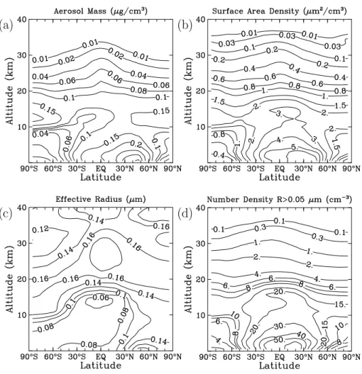
( ) (d)
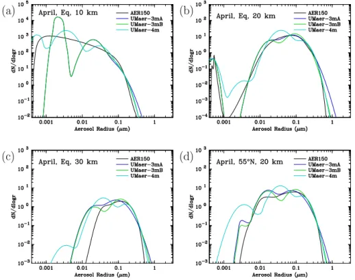
Fig. 3. Calculated size distributions from the AER 2-D model using the 150-bin sectional aerosol module AER150 (black lines), the 40-bin
sectional aerosol module AER40 (red lines), and the 20-bin sectional aerosol module AER20 (yellow lines) in April at (a) the equator and 10 km, (b) the equator and 20 km, (c) the equator and 30 km, and (d) 55◦N and 20 km.
carbon, and black carbon and cannot be compared with ob-servations. The stratospheric aerosol is realistic a few kilo-meters away from the tropopause, and will be compared with global observations from the SAGE II satellite. In Fig. 1 we show calculated annual average aerosol properties from the
AER150 model version for the global domain from the sur-face to 40 km (the top of the aerosol layer). Aerosol mass density in µg/m3, including both sulfuric acid and water in particulate form, is shown in Fig. 1a, and surface area density in µm2/cm3 in Fig. 1b. These integrated aerosol quantities
(a) (b)
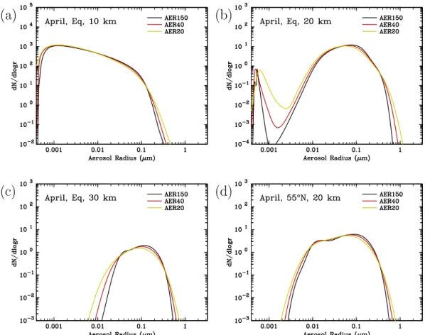
( ) (d)
Fig. 4. Percent change in model-calculated aerosol parameters from the AER 2-D model using the 40-bin sectional aerosol module AER40
versus the 150-bin sectional aerosol module AER150. Shown are annual average differences in (a) mass density, (b) surface area density, (c) effective radius, and (d) number density of particles with radius greater than 0.05 µm.
are important for mass balance and heterogeneous chemistry affecting ozone, respectively. Shown in Fig. 1c is the effec-tive radius, defined as
Reff= R r3 dN drdr R r2 dN drdr (8)
and in Fig. 1d the number density of particles with radii greater than 0.05 µm.
SAGE II version 6.1 observations of aerosol extinction at 1.02 and 0.525 µm are compared with AER150 extinctions, calculated by applying a Mie scattering code to the model-generated size distributions, in Fig. 2. The SAGE II data represent an average with gap-filling over the 2001–2002 period, as detailed in the SPARC aerosol assessment report (Thomason and Peter, 2006). The AER150 model produces calculated 1.02 µm extinctions well below the SAGE II ob-servations in the troposphere and tropopause region due to omission of non-sulfate aerosols, but within 30% of SAGE II observations in the stratosphere below 30 km. Calculated ex-tinctions above 30 km are significantly below observations,
and represent a combination of observational uncertainty and perhaps a poor representation of the evaporation pro-cess in the model. The comparison with 0.525 µm SAGE II extinction also shows agreement within 30% in the mid-stratosphere, but a different spatial pattern than the 1.02 µm extinction, indicating errors in model-representation of the size distribution. Uncertainties in model transport are also a factor in these comparisons. But the general agreement between the model and observations in the mid-stratosphere indicates a reasonable representation of sulfur sources and aerosol microphysics. Differences between the model ver-sions reported here are in many cases no greater than other model uncertainties, though these differences, caused by the representation of the size distribution, are shown to produce biases.
We compare the AER sectional modules with 40 bins (AER40) and 20 bins (AER20) with the sectional model us-ing 150 bins (AER150) to assess their accuracy relative to numerical diffusion in radius. Figure 3 shows calculated aerosol size distributions in April at several latitudes and
(a) (b)
( ) (d)
Fig. 5. Percent change in model-calculated aerosol parameters from the AER 2-D model using the 20-bin sectional aerosol module AER20
versus the 150-bin sectional aerosol module AER150. Shown are annual average differences in (a) mass density, (b) surface area density, (c) effective radius, and (d) number density of particles with radius greater than 0.05 µm.
(a)
(b)
Fig. 6. Percent change in annual average model-calculated aerosol mass density with sedimentation versus without sedimentation in the
AER40 model (panel a). Percent difference in annual average model-calculated aerosol mass density between the UMaer-3mA model without sedimentation and the AER40 model without sedimentation (panel b).
altitudes for the AER150 model, the AER40 model, and the AER20 model. The size distributions are very similar, but
lower resolution in size space produces more large particles and more small particles due to the size broadening effect
(a)
(b)
(c)
(d)
Fig. 7. Percent change in model-calculated annual average aerosol parameters from the AER 2-D model using the UMaer 3-mode aerosol
module UMaer-3mA versus the 150-bin sectional aerosol module AER150. Shown are annual average differences in (a) mass density, (b) surface area density, (c) effective radius, and (d) number density of particles with radius greater than 0.05 µm.
of numerical diffusion. At the equator and 20 km, shown in Fig. 3b, a nucleation mode is evident along with an accu-mulation mode. Size broadening in the AER40 and AER20 models leads to significantly more particles between the two modes.
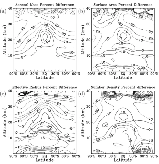
Figure 4 shows percent differences between AER40 and AER150 in aerosol mass density, surface area density, ef-fective radius, and number density. Aerosol mass den-sity between AER40 and AER150 is identical in the tropo-sphere, but in the stratosphere AER40 is reduced by 1% at the tropopause to 10–15% at 30 km relative to the AER150 model. The reduction in aerosol mass density with altitude is caused by greater sedimentation in AER40 with its slightly broader size distributions. AER40 also shows less surface area density than AER150, by 4–14% between the surface and 30 km. Reductions in the troposphere are seen due to differences in the size distributions between the two mod-els, even though their mass densities are the same. Effective radius is increased by 0–6% in AER40, consistent with the increase in large particles which leads to increased
sedimen-tation. Number density for particles greater than 0.05 µm radius is decreased by 8–12% throughout most of the tro-posphere and stratosphere. Figure 5 shows similar plots for the AER20 model relative to the AER150 model. Mass den-sity of the AER20 model is 5–30% smaller than the AER150 model in the stratosphere. Surface area density is 15–30% smaller. Effective radius is increased by 2–18%, and number density decreased by 25–30%.
We have run the AER40, AER20, 3mA, UMaer-3mB, and UMaer-4m models without sedimentation, since we expect that sedimentation will play a major role in dif-ferences between these models. Figure 6a shows the im-pact of sedimentation on aerosol mass density in the AER40 model. Sedimentation reduces aerosol mass by a few per-cent at the tropopause, up to 40% at 15 km, and up to 90% at 30 km. In the tropics below 25 km, aerosol mass is increased by sedimentation, since particles sediment from above into this region, and the upwelling circulation causes some par-ticles to stagnate here. Figure 6b shows a comparison of aerosol mass density calculated by the UMaer-3mA model
(a) (b)
( ) (d)
Fig. 8. Calculated size distributions from the AER 2-D model using the 150-bin sectional aerosol module AER150 (black lines), the 3-mode
UMaer-3mA aerosol module (blue lines), the 3-mode UMaer-3mB aerosol module (green lines), and the 4-mode UMaer-4m aerosol module (cyan lines) in April at (a) the equator and 10 km, (b) the equator and 20 km, (c) the equator and 30 km, and (d) 55◦N and 20 km.
without sedimentation versus the AER40 model without sed-imentation. In all of our comparisons, we adjust the radii of modal distributions to include condensed water, since the sectional model size distributions include both water and sul-fate. Differences between the models without sedimentation are 0–20% within the stratosphere below 35 km, and less than 5% in the troposphere. Over most of the model domain, the UMaer-3mA model without sedimentation calculated more aerosol mass density than the AER40 model without sedi-mentation. The UMaer-3mB model does not differ substan-tially from the Umaer-3mA model without sedimentation. The UMaer-4m model differs from the Umaer-3mA model by 2% or less in aerosol mass density in the lower strato-sphere when sedimentation is omitted. The AER20 model without sedimentation does not differ from the AER40 model below 35 km.
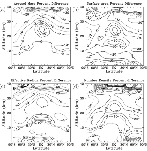
When sedimentation is included in the calculations, dif-ferences between the modal and sectional models become considerably larger. Figure 7a shows percent differences in aerosol mass density between models UMaer-3mA and AER150. The models don’t differ in the troposphere, but the UMaer-3mA model calculates less aerosol mass in most of the middle stratosphere, by as much as 40%. In the tropi-cal lower stratosphere, the UMaer-3mA model tropi-calculates up to 20% more aerosol mass, and near the tropopause at high latitudes up to 10% more aerosol mass. In the comparison
without sedimentation, the UMaer-3mA model showed an increase of 5–10% in aerosol mass over most of the strato-sphere relative to AER40. Sedimentation is removing more aerosol mass in the middle stratosphere of the UMaer-3mA model than in the AER150 model, and the excess sedi-mentation is increasing aerosol mass in parts of the lower stratosphere. Since an entire mode sediments at one rate, the modal model behaves differently than a low-resolution sectional model. Changes in surface area density between Umaer-3mA and AER150 are show in Fig. 7b. Surface area changes in both the troposphere and stratosphere, with dif-ferences within 20% everywhere except at high latitudes and high altitudes. Figure 7c shows differences in effective ra-dius, which is lower than AER150 by up to 30% at 30 km, and greater by up to 20% in the tropical upper troposphere and lower stratosphere. Number density, shown in Fig. 7d, is lower than AER150 by 10–20% in most of the stratosphere and up to 30% in the troposphere, but greater by 10% in the tropical lower stratosphere.
The aerosol size distributions generated by the modal models are shown in Fig. 8 for several latitudes and alti-tudes and compared with size distributions generated by the AER150 model. The blue lines represent the UMaer-3mA model and the green lines the UMaer-3mB model. These are both 3-mode models and differ only in the width of the third and largest mode. As seen in the figures, UMaer-3mA
(a)
(b)
(c)
(d)
Fig. 9. Percent change in model-calculated annual average aerosol parameters from the AER 2-D model using the UMaer 3-mode aerosol
module UMaer-3mB versus the 150-bin sectional aerosol module AER150. Shown are annual average differences in (a) mass density, (b) surface area density, (c) effective radius, and (d) number density of particles with radius greater than 0.05 µm.
always produces more large particles than UMaer-3mB and both produce more large particles than AER150 for the lo-cations shown. The 4-mode UMaer-4m model results are shown with cyan lines. The size distributions that the modal model is capable of reproducing accurately depend on the imposed number of modes and widths of those modes. The distribution shown in Fig. 8b for 20 km at the equator in April is a lognormal distribution of aged aerosol particles centered at about 0.1 µm with a secondary peak below 0.001 µm due to nucleation. The 3-mode models reproduce this distribu-tion well. The 4-mode model calculates too many particles in the 0.001 to 0.004 µm size range. The distribution shown in Fig. 8a for the tropical upper troposphere contains large numbers of particles from 0.0005 µm to 0.1 µm and results from continual nucleation. The 3-mode models cannot repro-duce this distribution over the full range of radii, but capture the distribution well for particles greater than 0.01 µm. The 4-mode model more accurately captures the particle distribu-tions for radii less than 0.01 µm. The distribudistribu-tions shown in Figs. 8c and d represent an aerosol population that may have
been subjected to evaporation or mixing of air masses with different histories. Both the 3-mode and 4-mode models have difficulty reproducing the lower size cutoff of these distribu-tions, with the 3-mode models performing better. However, since integrated aerosol properties depend most strongly on the larger particles in the distribution, this failure may not be significant for many applications.
Figure 9 shows percent changes in integrated aerosol prop-erties for the UMaer-3mB model relative to the AER150 model. This figure can be compared with Fig. 7 to evalu-ate how the width of the large mode in the 3-mode model affects quantities such as aerosol mass density and effective radius. The narrower width of the large mode in UMaer-3mB does lead to an aerosol mass density above 25 km which is closer to the AER150 mass density than the UMaer-3mA model. Mass density is still 10–30% less than AER150, but not 20–40% less as was UMaer-3mA. In the lower strato-sphere and up to 25 km in the tropics, the aerosol mass den-sity is greater than in AER150 and up to 10% greater than with UMaer-3mA. Narrowing the large mode of the 3-mode
(a)
(b)
(c)
(d)
Fig. 10. Percent change in model-calculated annual average aerosol parameters from the AER 2-D model using the UMaer 4-mode aerosol
module UMaer-4m versus the 150-bin sectional aerosol module AER150. Shown are annual average differences in (a) mass density, (b) surface area density, (c) effective radius, and (d) number density of particles with radius greater than 0.05 µm.
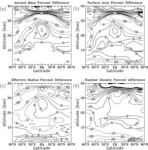
model improved the simulation of mass density in the mid-dle stratosphere but made the results somewhat worse in the lower stratosphere and tropics. The same is true for sur-face area density, where in addition the tropospheric values became somewhat worse. Effective radius, however, is im-proved in the entire stratosphere, but not in the troposphere. Calculated number density is improved in most of the tropo-sphere but becomes worse in the tropical stratotropo-sphere.
The same comparisons for the 4-mode model are shown in Fig. 10. The maximum difference between UMaer-4m and AER150 is only 20% in aerosol mass density or surface area density below 30 km. Large differences above that altitude are not significant in terms of stratospheric aerosol mass, but reflect differences in how the models simulate evaporation of aerosols at the top of the aerosol layer. Overall, the simula-tion of effective radius is quite good between 5 and 30 km. Number density simulations are also improved over the 3-mode 3-models, with only 10% differences in the stratosphere below 25 km, but with differences of 10–40% in the lower and middle troposphere.
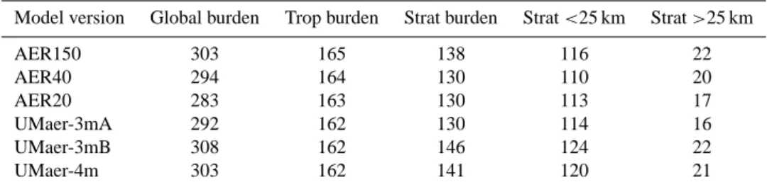
Table 2 gives the global aerosol burdens of the six simu-lations discussed, along with tropospheric and stratospheric burdens. The AER150 model predicts 165 kilotons of aerosol sulfur in the troposphere and 138 kilotons of sulfur in the stratosphere. The AER40 and AER20 models predicts 1% less in the troposphere and 6% less in the stratosphere. The modal models all predict 162 kilotons of sulfur in the tropo-sphere, but stratospheric burdens range from 130 to 146 kilo-tons. The UMaer-4m model predicts 141 kilotons of sulfur in the stratosphere, only 2% higher than the AER150 model. The 3mA model predicts 6% low and the UMaer-3mB model 6% high. Table 2 also shows a breakdown in stratospheric aerosol between that above and below 25 km. The AER150 model produces a stratospheric aerosol mass distribution with 16% above 25 km. The AER40, UMaer-3mB and UMaer-4m models have 15% of the stratospheric sulfate aerosol above 25 km, the AER20 model only 13%, and the UMaer-3mA only 12%. Though the global aerosol mass in the UMaer-4m model is closer to the AER150 model than is AER40, the AER40 model has smaller deviations
Table 2. Aerosol burdens in kilotons of sulfur calculated by each model version.
Model version Global burden Trop burden Strat burden Strat <25 km Strat >25 km
AER150 303 165 138 116 22 AER40 294 164 130 110 20 AER20 283 163 130 113 17 UMaer-3mA 292 162 130 114 16 UMaer-3mB 308 162 146 124 22 UMaer-4m 303 162 141 120 21
from AER150 at most latitudes and altitudes (see Figs. 4 and 10) in mass, surface area density, effective radius, and num-ber density. We find that a 4-mode model in general does a better job than a mode model, but in some situations a 3-mode 3-model simulates the size distributions better. The low resolution sectional model AER20 generally does a worse job than UMaer-4m and UMaer-3mB in our background at-mosphere simulations, though its differences from AER150 are more consistent spatially.
5 Volcanic perturbation intercomparison
We have simulated the Mt. Pinatubo volcanic eruption in the Phillipines in order to compare the different model formu-lations under very high aerosol loading and to compare the rates of aerosol decay. Our simulations are performed by in-jecting 20 megatons of SO2(Bluth et al., 1992; McCormick
et al., 1995) on 14 June 1991 into the tropical stratosphere be-tween 5◦S and 15◦N at 16–29 km altitude (Read et al., 1993). The simulations cover the 8 year period from the beginning of 1991 until the end of 1998. Simulations are performed with the AER40 model, the AER20 model, and the UMaer-3mA, UMaer-3mB, and UMaer-4m models. The AER40 model is used here as the benchmark model, since running the AER150 model for 8 years is not practical. Observations of aerosol extinction and surface area density derived from the SAGE II satellite are available during the growth and de-cay of Pinatubo aerosols, though the tropical lower strato-sphere experienced instrument saturation in the early months and observatons there are lacking.
Figure 11 shows model results of the evolution of 1.02 µm extinction from 1991 until 1999, as well as the SAGE II version 6.1 extinction observations. All models yield sim-ilar peak extinction values 2–3 months after the eruption in the tropics. This similarity is not unexpected, as the chemical transformation of SO2 to H2SO4 is independent
of the microphysical scheme, and thermodynamics dictate that all gas phase H2SO4 in the lower and middle
strato-sphere will condense into particles, though the condensation rate depends somewhat on the existing particle size distribu-tion. Between 1992 and 1996, the AER40, AER20, UMaer-3mB, and UMaer-4m models match observations adequately
(a)
(b)
Fig. 11. Aerosol extinction at 1.02 µm in km−1for 1991 to 1999 at (a) the equator and 26 km, and (b) 55◦N and 20 km. SAGE II data version 6.1 are shown by black symbols with error bars, model results by colored lines.
at the equator and 26 km. The UMaer-3mA model results are much too low between 1992 and 1996, a results of the excessive width of the largest mode which leads to excess sedimentation. The two sectional models and UMaer-4m match each other closely, with UMaer-3mB yielding some-what lower values of extinction between 1992 and 1996. The
(a)
(b)
Fig. 12. Aerosol surface area density in µm2/cm3for 1991 to 1999 at (a) the equator and 26 km, and (b) 55◦N and 20 km. SAGE II data version 6.1 are shown by black symbols with error bars, model results by colored lines.
UMaer-3mB model matches observations best in late 1992 and early 1993, but AER40, AER20, and UMaer-4m match more closely between mid-1993 and 1997. After 1997, the modal model results are higher than the sectional model re-sults and the observations. Rere-sults at 55◦N and 20 km are also shown in Fig. 11. The SAGE II observations have larger error bars here, and the models show larger differences due to the transport time from the tropics and the differences in sedimentation and size evolution during this period. Peak extinction in early to mid 1992 differs among the models, with the UMaer-3mA model reaching only 1/3 the maximum of the AER40 model. We find that the UMaer-3mA model matches observations most closely in 1992, and UMaer-3mB matches most closely in 1994 and 1995. The sectional mod-els are significantly higher than observations in these years, perhaps due to a poor representation of the initial SO2
dis-tribution from the eruption or to inadequacies in the model transport.
(a)
(b)
Fig. 13. Aerosol effective radius in µm for 1991 to 1999 at (a)
the equator and 26 km, and (b) 55◦N and 20 km from simulations with the AER40, AER20, 3mA, 3mB, and UMaer-4m models.
The evolution of modeled aerosol surface area density at the equator and 26 km and at 55◦N and 20 km is shown in Fig. 12. Surface area density derived from SAGE II ver-sion 6.1 extinction observations, as described in Thomason and Peter (2006), is also shown. Surface area density appears less sensitive to model formulation than extinction or mass density, with all models except UMaer-3mA showing almost coincident results which match observations well between 1992 and 1994 at the equator and 26 km. After 1995, the sec-tional models calculate lower surface area densities than do any of the UMaer models. At 55◦N and 20 km, UMaer-3mA results lie significantly below those of the other models and match the observations most closely during 1992 and 1993, while UMaer-4m produces the highest reslts, sometimes well above observations. The AER20 model produces the low-est surface area density after 1995, though error bars in the observations eliminate only the UMaer-3mB and UMaer-4m models. We have not found a single model version which best match observations at all latitudes, altitudes, and times,
(a) (b)
( ) (d)
Fig. 14. Calculated size distributions from simulations of the Mt. Pinatubo eruption using the AER 2-D model with the 40-bin sectional
aerosol module AER40 (red lines), the UMaer-3mA module (blue lines), the UMaer-3mB module (green lines) and the UMaer-4m module (cyan lines) at (a) the equator and 26 km in January 1992, (b) the equator and 26 km in January 1994, (c) 55◦N and 20 km in January 1992, and (d) 55◦N and 20 km in January 1994.
illustrating that uncertainties in model dynamics may dwarf the accuracy of the microphysics scheme.
The time evolution of aerosol effective radius is shown in Fig. 13. This parameter is sensitive to the full particle size spectrum, unlike extinction and surface area density which depend mostly on the larger particles which contain the ma-jority of the aerosol mass. The effect of a large increase in gas phase sulfur in the stratosphere is to produce a burst of nucleation, seen here as a drop in effective radius at the time of the eruption, and then to increase particle sizes over sev-eral months, from about 0.15 µm to about 0.45 µm, as the vast majority of sulfur condenses onto existing particles and increases their diameters. As shown in Fig. 14, the AER40 model calculates a narrower size distribution than the modal models in the post-Pinatubo period. The modal models have aerosol mass mainly in the largest mode whose width is spec-ified and wider than that calculated by AER40. The AER40 size distributions are not symmetrical in January 1992 or January 1994, peaking at 0.4–0.5 µm and dropping faster on the high radius side than on the low radius side. The modal models generate far more particles below 0.1 µm
ra-dius, and thus produce a smaller effective radius. Distribu-tions from the AER20 model are very similar to but slightly wider than AER40 and are not shown in the figure. Effective radius at the equator and 26 km is up to 40% low in UMaer-3mA relative to AER40 in 1994 and 1995, and falls back to background levels 2 years sooner than AER40. UMaer-3mB does a somewhat better jobs than UMaer-3mA but still calculates much lower effective radii and an earlier return to background conditions. The UMaer-4m model does a bet-ter job of simulating effective radius, but is still 17% low in 1994. The AER20 model simulates effective radius quite ac-curately between 1992 and 1996, much better than any of the modal models.
The rate at which the particulate matter is removed from the stratosphere is a function of sedimentation rate, which depends on the amount of aerosol mass in larger particles. Thus the different microphysical schemes calculate some-what different rates of aerosol decay following this simu-lated volcanic injection. Models 3mA and UMaer-3mB differ only in the width of the largest lognormal mode, and show aerosol decay at very different rates, confirming the
importance of the large particle distribution to sedimentation rates. The decay rate of extinction for UMaer-3mB is some-what faster than for AER40, but the UMaer-3mA model de-cays much too fast. The UMaer-4m model gives decay rates close to the AER40 model for the 1992–1995 period. The AER20 low-resolution sectional model also performs well during the post-Pinatubo period, and calculates effective ra-dius much better than any of the modal models. This high-lights the deficiency of a modal model, which forces sedi-mentation of all mass in an aerosol mode at the same rate.
6 Conclusions
We have performed global 2-D model calculations with three versions of a sectional model and three versions of a modal model. The sectional model with 40 bins has numerical dif-fusion compared to the sectional model with 150 bins, result-ing in somewhat greater sedimentation and 6% less strato-spheric aerosol mass, with maximum differences of 15% at 30 km. We tested two three-mode model versions and found a 12% difference between them in stratospheric aerosol mass as a function of the prescribed width of the largest lognor-mal mode. Differences in aerosol mass between these mod-els and the 150-bin sectional model are as high as 40% at 30 km. A four-mode version was found to perform better than the three-mode version under some, but not all, condi-tions. A low-resolution sectional model with 20 bins was found to be very efficient but roughly comparable in accu-racy to the UMaer-3mB model for a background atmosphere calculation. Effective radius was more sensitive to model for-mulation than mass density or surface area density.
Our 8-year calculations of the Pinatubo eruption period have been compared with SAGE-II observations of aerosol extinction at 1.02 µm and show that the UMaer-3mA ver-sion indeed has sedimentation which removes aerosol mass too quickly. The AER40, AER20, 3mB and UMaer-4m versions are all generally consistent with observations be-tween 1992 and 1996, but the sectional models better match observations after 1996 when background aerosol levels are approached. We have not found a single model version which best match observations at all latitudes, altitudes, and times, indicating the importance of other model uncertainties. Cal-culated effective radius shows the clearest distinction be-tween model versions during the 1992–1996 period, and the AER20 model is found to match the more accurate AER40 model quite well for this quantity.
Based on the model performances documented here and the computational efficiency, we recommend that the AER40 and UMaer-3mB model versions should be incorporated into the GMI stratosphere-troposphere chemistry-transport model. In addition, the low-resolution AER20 sectional model could be useful for certain applicatons. Developing a modal model which can prognostically determine mode
width would likely be more efficient computationally and at least as accurate as a 4-mode scheme without this feature.
Acknowledgements. This work was supported by the NASA
Atmospheric Chemistry Modeling and Analysis Program and the NASA Modeling Anaylsis and Prediction program.
Edited by: A. Nenes
References
Bekki, S. and Pyle, J. A.: 2-D assessment of the impact of aircraft sulphur emissions on the stratospheric sulphate aerosol layer, J. Geophys. Res., 97, 15 839–15 847, 1992.
Bluth, G. J. S., Doiron, S. D., Schnetzler, C. C., Krueger, A. J., and Walter, L. S.: Global tracking of the SO2clouds from the
June 1991 Mount Pinatubo eruptions, Geophys. Res. Lett., 19, 151–154, 1992.
Carslaw, K. S., Luo, B., and Peter, Th.: An analytic expression for the composition of aqueous HNO3-H2SO4stratospheric aerosol
including gas phase removal of HNO3, Geophys. Res., Lett., 22,
1877–1880, 1995.
Considine, D. B., Douglass, A. R., Connell, P. S., Kinnison, D. E., and Rotman, D. A.: A polar stratospheric cloud parameterization for the three-dimensional model of the global modeling initiative and its response to stratospheric aircraft emissions, J. Geophys. Res., 105, 3955–3975, 2000.
Douglass, A. R., Prather, M. J., Hall, T. M., Strahan, S. E., Rasch, P. J., Sparling, L. C., Coy, L., and Rodriguez, J. M.: Choosing me-teorological input for the global modeling initiative assessment of high-speed aircraft, J. Geophys. Res., 104, 27 545–27 564, 1999.
Douglass, A. R., Connell, P. S., Stolarski, R. S., and Strahan, S. E.: Radicals and reservoirs in the GMI chemistry and transport model: comparison to measurements, J. Geophys. Res., 109, D16302, doi:10.1029/2004JD004632, 2004.
Fahey, D. W., Kawa, S. R., Woodbridge, E. L., et al.: In situ measurements constraining the role of sulphate aerosols in mid-latitude ozone depletion, Nature, 363, 509–514, 1993.
Fleming, E. L., Jackman, C. H., Stolarski, R. S., and Considine, D. B., Simulation of stratospheric tracers using an improved empirically-based two-dimensional model transport formulation, J. Geophys. Res., 104, 23 911–23 934, 1999.
Hall, T. M., Waugh, D. W., Boering, K. A., and Plumb, R. A.: Evaluation of transport in stratospheric models, J. Geophys. Res., 104, 18 815–18 839, 1999.
Hansen, D., Sato, M., Nazarenko, L., et al.: Climate forcings in the Goddard Institute for Space Studies SI2000 simulations, J. Geo-phys. Res., 107, D17, 4347, doi:10.1029/2001JD001143, 2002. Haywood, J. and Ramaswamy, V.: Global sensitivity studies of the
direct radiative forcing due to anthropogenic sulphate and black carbon aerosols, J. Geophys. Res., 103, 6043–6058, 1998. Herzog M., Weisenstein, D. K., and Penner, J. E.: A
dy-namic aerosol module for global chemical transport mod-els: Model description, J. Geophys. Res., 109, D18202, doi:10.1029/2003JD004405, 2004.
Hofmann, D. J. and Solomon, S.: Ozone destruction through het-erogeneous chemistry following the eruption of El Chichon, J. Geophys. Res., 94, 5029–5041, 1989.
Jackman, C. H., Douglass, A. R., Brueske, K. F., and Klein, S. A.: The influence of dynamics on two-dimensional model results: Simulations of14C and stratospheric aircraft NOxinjections, J.
Geophys. Res., 96, 22 559–22 572, 1991.
Jacobson, M. Z.: Global direct radiative forcing due to multicompo-nent anthropogenic and natural aerosols, J. Geophys. Res., 106, 1551–1568, 2001.
Kalnay, E., Kanamitsu, M., Kistler, R., et al.: The NCEP/NCAR 40-year reanalysis project, Bull. Am. Meteorol. Soc., 77, 437–471, 1996.
Kinnison, D. E., Connell, P. S., Rodriguez, J. M., et al.: The Global Modeling Initiative assessment model: Application to high-speed civil transport perturbation, J. Geophys. Res., 106, 1693–1711, 2001.
Labitzke, K. and McCormick, M. P.: Stratospheric temperature in-creases due to Pinatubo aerosols, Geophys. Res. Lett., 19, 207– 210, 1992.
Liu X., Penner, J. E., and Herzog, M.: Global modeling of aerosol dynamics: Model description, evaluation, and interactions be-tween sulfate and nonsulfate aerosols, J. Geophys. Res., 110, D18206, doi:10.1029/2004JD005674, 2005.
McCormick, M. P., Thomason, L. W., and Trepte, C. R.: Atmo-spheric effects of the Mt. Pinatubo eruption, Nature, 373, 399– 404, 1995.
Mills, M. J., Toon, O. B., Solomon, S. S.: A two-dimensional mi-crophysical model of the polar stratospheric CN layer, Geophys. Res. Lett., 26, 1133–1136, 1999.
Newell, R. E., Kidson, J. W., Vincent, D. G., and Boer, G. J.: The General Circulations of the Tropical Atmosphere, vol. 2, MIT Press, Cambridge, Mass., 1974.
Penner, J. E., Andreae, M., Annegarn, H., et al.: Aerosols: Their direct and indirect effects, in: Climate Change 2001: The Scien-tific Basis, edited by: Houghton, H. T., Ding, Y., Griggs, D. J., et al., pp. 289–348, Cambridge Univ. Press, New York, 2001. Penner, J. E., Zhang, S. Y., Chin, M., et al.: A comparison of model
and satellite-derived aerosol optical depth and reflectivity, J. At-mos. Sci., 59, 441–460, 2002.
Pitari, G., Mancini, E., Rizi, V., and Shindell, D. T.: Impact of fu-ture climate and emission changes on stratospheric aerosols and ozone, J. Atmos. Sci., 59, 414–440, 2002.
Randel, W. J. and Garcia, R. R.: Application of a planetary wave breaking parameterization to straospheric circulation statistics, J. Atmos. Sci., 51, 1157–1168, 1994.
Read, W. G., Froidevaux, L., and Waters, J. W.: Microwave limb sounder measurements of stratospheric SO2from the Mt.
Pinatubo volcano, Geophys. Res. Lett., 20, 1299–1302, 1993. Rosenfield, J. E., Newman, P. A., and Schoeberl, M. R.:
Computa-tion of diabatic descent in the stratospheric polar vortex, J. Geo-phys. Res., 99, 16 677–16 689, 1994.
Rotman, D. A., Tannahill, J. R., Kinnison, D. E., et al.: The Global Modeling Initiative Assessment Model: Model description, inte-gration and testing of the transport shell, J. Geophys. Res., 106, 1669–1691, 2001.
Sander, S. P., Friedl, R. R., DeMore, W. B., et al.: Chemical ki-netics and photochemical data for use in stratospheric modeling, Supplement to evaluation 12: Update of key reactions, Evalua-tion Number 13, JPL PublicaEvalua-tion 00-3, Jet Propulsion Labora-tory, NASA, 2000.
Seinfeld, J. H. and Pandis, S. N.: Atmospheric Chemsitry and Physics, John Wiley, Hoboken, N.J., 1997.
Smolarkiewicz, P. K.: A simple positive definite advection scheme with small implicit diffusion, Mon. Wea. Rev., 111, 479–487, 1984.
Stier, P., Feichter, J., Kinne, S., et al.: The aerosol-climate model ECHAM5-HAM, Atmos. Chem. Phys., 5, 1125–1156, 2005, http://www.atmos-chem-phys.net/5/1125/2005/.
Strahan, S. E. and Douglass, A. R.: Evaluating the credibility of transport processes in simulations of ozone recovery using the Global Modeling Initiative three-dimensional model, J. Geophys. Res., 109, D05110, doi:10.1029/2003JD004238, 2004.
Tabazadeh, A., Toon, O. B., Clegg, S. L., and Hamill, P.: A new parameterization of H2SO4/H2O aerosol composition:
Atmo-spheric implications, Geophys. Res., Lett., 24, 1931–1934, 1997. Thomason, L. and Peter, Th. (Eds.): SPARC Assessment of Strato-spheric Aerosol Properties, WCRP-124, WMO/TD NO. 1295, SPARC Report No. 4, Toronto, Canada, 2006.
Timmreck, C.: Three-dimensional simulation of stratospheric back-ground aerosol: First results of a multiannual general circulation model simulation, J. Geophys. Res., 106, 28 313–28 332, 2001. Vehkam¨aki, H., Kulmala, M., Napari, I., Lehtinen, K. E. J.,
Timm-reck, C., Noppel, M., and Laaksonen, A.: An improved parame-terization for sulfuric acid-water nucleation rates for tropospheric and stratospheric conditions, J. Geophys. Res., 107(D22), 4622, doi:10.1029/2002JD002184, 2002.
Weisenstein, D. K., Yue, G. K., Ko, M. K. W., Sze, N. D., Ro-driguez, J. M., and Scott, C. J.: A two-dimensional model of sul-fur species and aerosol, J. Geophys. Res., 102, 13 019–13 035, 1997.
Weisenstein, D. K., Ko, M. K. W., Dyominov, I. G., Pitari, G., Ric-ciardulli, L., Visconti, G., and Bekki, S.: The effects of sulfur emissions from HSCT aircraft: A 2-D model intercomparison, J. Geophys. Res., 103, 1527–1547, 1998.
Wennberg, P. O., Cohen, R. C., Stimpfle, R. M., et al.: Removal of stratospheric O3by radicals: In situ measurements of OH, HO2,
NO, NO2, ClO, and BrO, Science, 266, 398–404, 1994. Wilson, J., Cuvelier, C., and Raes, F.: A modeling study of global
mixed aerosol fields, J. Geophys. Res., 106, 34 081–34 108, 2001.
Wright, D. L., Kasibhatla, P. S., McGraw, R., and Schwartz, S. E.: Description and evaluation of a six-moment aerosol microphysi-cal module for use in atmospheric chemimicrophysi-cal transport models, J. Geophys. Res., 106, 20 275–20 291, 2001.
WMO: Scientific Assessment of Ozone Depletion: 1991, World Meteorological Organization Global Ozone Research and Moni-toring Project Report No. 25, Geneva, 1992.
Zhang, Y., Pun, B., Vijayaraghavan, K., Wu, S.-Y., Seigneur, C., Pandis, S. N., Jacobson, M. Z., Nenes, A., and Seinfeld, J. H.: Development and application of the model of aerosol dynam-ics, reaction, ionization, and dissolution (MADRID), J. Geophys. Res., 109, D01202, doi:10.1029/2003JD003501, 2004.

![[PDF] Introduction à la programmation orientée objet en Delphi | Cours informatique](data:image/gif;base64,R0lGODlhAQABAIAAAP///wAAACH5BAEAAAAALAAAAAABAAEAAAICRAEAOw==)