HAL Id: insu-00344313
https://hal-insu.archives-ouvertes.fr/insu-00344313
Submitted on 12 Jan 2010HAL is a multi-disciplinary open access archive for the deposit and dissemination of sci-entific research documents, whether they are pub-lished or not. The documents may come from teaching and research institutions in France or abroad, or from public or private research centers.
L’archive ouverte pluridisciplinaire HAL, est destinée au dépôt et à la diffusion de documents scientifiques de niveau recherche, publiés ou non, émanant des établissements d’enseignement et de recherche français ou étrangers, des laboratoires publics ou privés.
Emmanuel Le Trong, Olivier Rozenbaum, Jean-Louis Rouet, Ary Bruand
To cite this version:
Emmanuel Le Trong, Olivier Rozenbaum, Jean-Louis Rouet, Ary Bruand. A simple methodology to segment X-ray tomographic images of a multiphasic building stone.. Image Analysis and Stereology, International Society for Stereology, 2008, 27, pp.175-182. �insu-00344313�
X-RAY TOMOGRAPHIC IMAGES OF A
MULTIPHASIC BUILDING STONE.
by
Emmanuel Le Trong, Olivier Rozenbaum, Jean-Louis Rouet
and Ary Bruand
Institut des Sciences de la Terre d’Orl´eans, UMR 6113 - CNRS/Universit´e
d’Orl´eans, 1a, rue de la F´erollerie, 45071 ORL ´
EANS Cedex 2
E-mail: [email protected]
Abbreviated running title: Segmentation of micro-tomographic images
Abbreviated authors:
Le Trong E et al.
Key words:
alternate sequential filter, building stone
mathematical morphology,
segmentation,
watershed, X-ray tomography
ABSTRACT
Assessment of the weathering of a particular limestone, the tuffeau, used in historical monuments requires an accurate description of its microstructure. An efficient tools to obtain such a description is X-ray microtomography. However the segmentation of the images of this multiphasic material is not trivial. As the identification of pertinent markers of the structural components to extract is difficult, a two steps filtering approach is chosen. Alternate sequential filters are shown to efficiently remove the noise but, as they destroy the structural components smaller than the structuring element used, they cannot be carried out far enough. Hence as a second step in the filtering process, a mosaic operator, relying on a pragmatic yet efficient marker determination, is implemented to simplify further the images.
INTRODUCTION
Exposed to their climatic environment, the building stones of heritage monuments are often altered and eventually destroyed. This phenomenon called weathering is visible throughout the world and many studies in this field, led with architects and restorers, aimed at finding processes to slow down, control or ultimately avoid this decay (Amoroso and Fassina, 1983; Tiano et al., 2006; Torraca, 1976). A way to achieve such a goal is to understand the weathering mechanisms of building stones, i.e. to relate the microscopic mechanisms occurring at the pore scale (dissolution of minerals, transport, precipitation, etc.) to their consequences at the macro-scale (desquamation, powdering, etc.) (Amoroso and Fassina, 1983; Camuffo, 1995; T¨or¨ok, 2002). Some studies comparing weathered stones with unweathered stones were performed. The chemical and mineralogical com-position, as well as the porosity were analyzed (Rozenbaum et al., 2007; Maravelaki-Kalaitzaki et al., 2002; Galan et al., 1999). The main processes of weathering were thus qualitatively inferred from the identified differences. However, a more quantitative understanding of these weathering mechanisms and their consequences is to simulate them via a computerized model. This requires in turn a quantitative, realistic description of the three dimensional structure of the porous medium (Dullien, 1992; Adler, 1992; Anguy et al., 2001). An increasingly developing technique to achieve such a goal is X-ray tomography which produces 3-d images related to the absorption coefficients of the various phases constituting the material (Kak and Slaney, 2001). In this contribution the images have been acquired on the ID-19 micro-tomographic beamline at the European Synchrotron Radiation Facility. These facilities have several advantages compared to desktop devices : smaller pixel size, X-ray beam quality (monochromaticity, stability, high flux) that lead to high quality and high resolution images Baruchel et al. (2006). However the segmentation of a raw tomographic image is seldom a trivial process, highly dependent on the starting image and the objects to extract from it. Segmentation is the process of partitioning billions of gray-level voxels of a 3-d image into distinct objects or phases. The goal, in the context of building stones, is be to separate the void phase from
some distinct solid phases (two for the stone under study). Most of the segmentation complexity is related to the presence of noise (voxels with the same gray value can actually belong to two different phases) and blur (the borders between the phases are not well defined). Moreover, because the images are big and three-dimensional, the analysis cannot be done by hand (e.g. by marking the objects of interest) and must be as automated as possible. The main techniques found in the literature are:
– Thresholding the gray levels histogram, with (Kaestner et al., 2006) or without (Ap-poloni et al., 2007) a former filtering, with automatically (Sezgin and Sankur, 2004) or manually (Appoloni et al., 2007) determined thresholds. The thresholded images sometimes have to undergo a binary post-treatment to adjust the results of these approaches. Most of the time it is a reconstruction of the connected components of interest (du Roscoat et al., 2005; Lambert et al., 2005; Kaestner et al., 2006; Erdogan et al., 2006; Ketcham, 2005).
– Active contours on the image considered as a level set (Ramlau and Ring, 2007; Chung and kin Ho, 2000; Maksimovic et al., 2000; Qatarneh et al., 2001). These techniques are mostly used in medical applications and usually require some a
priori knowledge of the locations of the interfaces.
– Watershed-based techniques (Beucher and Lantuejoul, 1979; Beucher et al., 1990; Beucher, 1992; Vachier and Meyer, 2005; Videla et al., 2007; Malcolm et al., 2007; Benouali et al., 2005; Carminati et al., 2006). These techniques allow the extraction of individually marked objects.
– Combined techniques, e.g. (Sheppard et al., 2004).
The subject of this contribution is to provide a segmentation methodology of the images of a limestone described hereafter. The technique used falls into the first category, i.e. filtering followed by thresholding. Nevertheless one of the filters used is the mosaic operator, based on a watershed Beucher (1990); Beucher et al. (1990). This methodology
has been developed because it does not require the marking of each object to be retrieved which appears difficult in this context of multiphased noisy images. Following this introduction, section 2 presents the stone used in this study that serves as model stone, the sample preparation, and the images obtained.
Section 3 details the image analysis procedure, based on mathematical morphology tools, used to segment the images. Section 4 concludes this contribution.
X-RAY MICRO-TOMOGRAPHY OF TUFFEAU
SAM-PLE
←insert Fig. 1←insert Fig. 2
Most heritage monuments (chˆateaux, churches, cathedrals or houses) constituting the cultural heritage of the Loire valley, that is registered to the World Heritage list of the UNESCO, are made with tuffeau, a highly porous limestone (porosity≈ 45%) originating
from this valley. Previous studies (Dessandier, 1995; Brunet-Imbault, 1999; Rozenbaum
et al., 2007) showed that minerals are essentially sparitic (large grains) or micritic (small
grains) calcite (≈50%), silica (≈45%) in the form of opal cristobalite-tridymite spheres
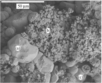
and quartz crystals, and some secondary minerals such as clays and micas in much smaller proportion (a few %). The scanning electron microscopic (SEM) image in figure 1 illustrates this structural variety, in shapes and sizes, of the main phases of tuffeau. X-ray tomography (Kak and Slaney, 2001) is a choice technology to extract the structure of samples of various porous materials: rocks (e.g. Lindquist and Venkatarangan (1999); Cnudde and Jacobs (2003); Cnudde et al. (2004); Sheppard et al. (2004); Appoloni et al. (2007); Betson et al. (2004; 2005); Videla et al. (2007)), cements and ceramics (e.g. Erdogan et al. (2006); Maire et al. (2007)), soils (e.g. Gryze et al. (2006); Carminati
et al. (2006)) and others (e.g. Jones et al. (2004); Mendoza et al. (2007); du Roscoat et al. (2005); Prodanovi´c et al. (2005)). Weathering of building stones has previously
been investigated by way of X-ray tomography (Cnudde and Jacobs (2003); Cnudde
two phases where under consideration, void and solid. The typical sizes of the smallest structural components of tuffeau relevant to our interest, like micritic calcite grains (a few
µm in size) and opal spheres (10 to 20µm in size), suggest the use of a high resolution tomograph, which leads toward synchrotron radiation facilities. However smaller struc-tures, such as those related to the opal spheres roughness or phyllosilicates, will not be accessible as their size is far below the best resolution any X-ray tomographic facility can achieve nowadays. The microtomographic images presented in this study were collected at the ID-19 beamline of the ESRF (European Synchrotron Radiation Facility, Grenoble, France) (Salvo et al., 2003; Baruchel et al., 2006) at the smallest possible pixel size (0.28 µm) the facility can reach. This pixel size compared to the size of the smallest structural components to be extracted allow a fair margin for the deployment of the image segmentation method. The energy used was 14.7 keV and 1500 successive rotations of the sample corresponding to 1500 angular positions ranging between 0◦ and 180◦ were acquired by the FReLoN camera with 2048× 2048 pixels image size. In order to stay in
the field of view of the detector and avoid supplementary artifacts, the samples have to measure less than 700 µm in diameter. They were prepared as cylindrical cores of that diameter and were mounted on a vertical rotator on a goniometric cradle. Preparation of a tuffeau sample of such a size requires particular care. Samples were impregnated with a resin in order to make a 700 µm thin section. This impregnation was necessary to keep the coherence of such small samples. Indeed the whole sample has to fit in the field of view of the X-ray beam to avoid artifacts. Local tomography (or region of interest tomography) will release this constraint but it is not yet operational at the ESRF. This latter was cut into matches of square section and finally trimmed to obtain quasi-cylinders of diameter ≈ 700µm. Imaging time was approximately 45 minutes and the 2048 horizontal slices (0.28 µm thick) were reconstructed from the projections with a dedicated filtered back-projection algorithm. The outputs of the tomographic process are then images of 2048× 2048 × 2048 voxels with 256 level gray level values (one
uncompressed image is then 8 GB in size). The gray level value of a voxel is linked to the X-ray absorption of the sample at the voxel position (Baruchel et al., 2000). Thus,
the pores appear in dark gray, the silica compounds in medium gray and the calcite compounds in light gray in figure 2. The different phases are easily distinguishable to the naked-eye: calcite is present in the form of large irregular grains (sparitic calcite) or small grains that look like crumble (micritic calcite); silica has the form of large quartz crystals or small spheres of opal. Nevertheless a direct threshold of the raw images is not possible considering their histogram (figure 4, red curve); one cannot identify the expected three peaks. This is due to the presence of noise as illustrated on figure 3-a, which clearly shows the impossibility to select two gray levels that would distinguish the three phases from each other.
TWO STEPS IMAGE FILTERING
Segmentation can be based on the automatic marking of each structural component to be extracted followed by the identification of the zone of influence of each marker (via a watershed operator (Beucher and Lantuejoul, 1979; Vincent and Soille, 1991)). This approach requires either the definition of markers based on a shape and/or size criterion Beucher et al. (1990) or markers based on a rough a priori knowledge of the gray level of the background and the foreground, possibly cleaned-up or merged by swamping (Beucher (1992)). From our point of view (i) the multiphasic nature, (ii) the variety of shapes and sizes of the structural components of each phase and (iii) the presence of noise, does not allow to propose a solid criterion for the identification of such markers. Hence segmentation can only rely on the gray level of each phase and thus our proposed method will consist of denoising the images, prior to a mere threshold. Classical denoising tools like linear (e.g. mean) or non-linear (e.g. median) filters are usually efficient but introduce a blur, which in turn has to be dealt with via some edge-enhancing techniques (e.g. janaki and ebenezer (2006)). The (noisy) images under con-sideration have a good sharpness (as illustrated on figure 3-a) one would like to preserve. Mathematical morphology (Matheron, 1975; Serra, 1982; 1988) proposes an efficient denoising tool called alternate sequential filters (ASF) that does not smooth images. It
is a sequence of alternate openings and closings with structuring elements of increasing sizes. Nevertheless the price to pay is the loss of any structural component smaller than the biggest (last) structuring element used. Hopefully the pixel size compared to the smallest structures to extract allow the use of such a filter, up to a certain size. This single filtering is shown to be insufficient in the subsequent section. A mosaic operator, i.e. a flattening of the zones of influence of carefully chosen markers transforms the image in an assemblage of flat (in a gray-level sense) zones, or mosaic, which can then be straightforwardly thresholded.
FILTERING WITH ASF
A 3-d image f is considered as a set of N× N × N voxels, N ∈ N, on a cubic grid with
26-neighboring, each having an integer value (its gray level), in the range[0,255].
f= {vi jk}, vi jk∈ [0,255], (i,j,k) ∈ [0,N− 1]. (1)
The image is here considered cubic for the sake of simplicity. Each voxel can be located in the image with a unique triplet of numbers (coordinates).
f(x) = vi jk, x= {i,j,k}. (2)
On a gray level image, the erosion ε and the dilation δ by a structuring element B are defined at every point x by Serra (1982)
δB(f)(x) = ∨ { f (x − y), y∈ B(x)} (3)
εB(f)(x) = ∧ { f (x − y), −y ∈ B(x)} (4)
where∨ if the supremum (or maximum) operator and ∧ the infimum (minimum) operator
and B(x) is the structuring element centered at point x. The openingγ and closingϕ are defined by the adjunctions Serra (1982)
γB = δBεB (5)
A particular family of digital balls Bλ, with radius λ, have been used for the structuring elements
Bλ(x) = {y, d(x,y) ≤λ}, λ ∈ N (7)
where d(x,y) is the euclidean distance between the centers of the two voxels at
coordi-nates x and y in voxel-size unit. This choice was made because these balls are a better approximation of the euclidean sphere than those based on the digital distance d26(which
are euclidean cubes) and they do not impact the efficiency of the implementation. The sequential alternate filtering are brought up toλ = 3, yielding the filtered image h
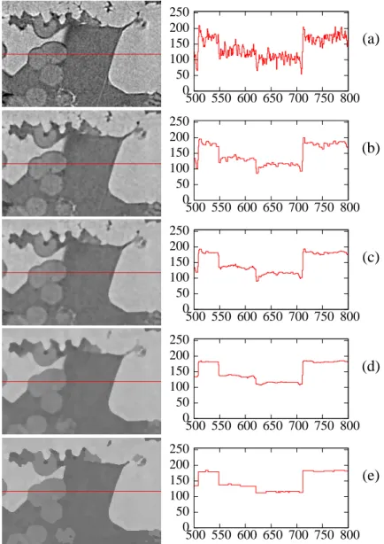
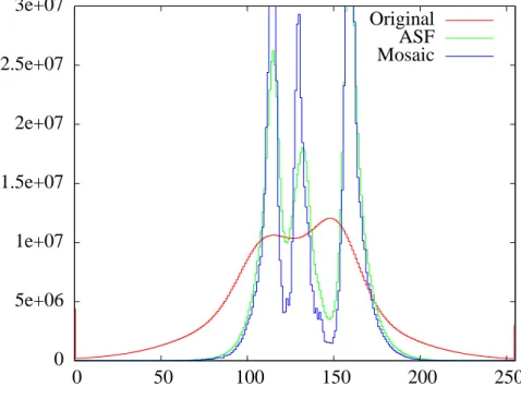
h=γB3ϕB3γB2ϕB2γB1ϕB1(f). (8) The intermediate steps and the result of this filtering operation are shown in figure 3-(a) to (d), on which the denoising power of the ASF is clearly visible. A structuring element withλ = 3 leads to a digital ball of 7 × 0.28= 1.96µm in diameter, which is compatible with the smallest elements to be identified in the images (micritic calcite). The result of the denoising appears clearly on the histogram of the filtered image in figure 4 (green curve); three peaks are neatly distinguished which allow an obvious threshold of the three phases. The thresholds are the gray values at which the histogram has a local minima. The results of such a threshold are illustrated on figure 5. For the ”simple” zone (left column) the result is acceptable but for a more ”complicated” zone, containing micritic calcite (right column) it is not. A lot of inexistent silica is artificially identified between
the calcite and the resin. ←insert Fig. 3
FILTERING WITH MOSAIC
In order to denoise the image further, it is possible to carry on ASF filtering with bigger structuring elements, but the loss of structural components of these sizes will not be acceptable. Another denoising operation is introduced, the mosaic. The mosaic operator was invented by Beucher (1990). The idea is to simplify the image in an assemblage zones of constant gray level. Beucher then originally performed a merging of neighboring
zones following a given criterion (hence performing a watershed operation on the graph of the connected zones, see Beucher (1990)), in order to simplify further the images. The idea here is simpler, the mosaic operator is merely viewed as an additional filtering step in order to remove more noise and improve the separation between the phases in terms of gray levels. The marker determination is a key feature of the method. After the filtering by ASF the image is already essentially composed of flat zones (see figure 3-(d)) each of which being a minima of the gradient of the image. The use of these minima as markers to build a mosaic leads to the creation of too many zones and does not simplify enough the image. In fact the mosaic constructed upon such a marker is very similar to the filtered image and does bring any improvement. In order to build a more efficient marking criterion, a strong assumption is made about the images: each separated structural component inside a given phase (e.g. a block of sparitic calcite, a small grain of micritic calcite or an isolated opal sphere) contains at least one local extremum (minimum or maximum). Inside a ”big” component (e.g. a block of sparitic calcite, an opal sphere) this assumes that there is still enough noise to create such local extrema, i.e. the zone is not completely flat. In which case, as it is likely to be surrounded by voxels of higher and lower gray value, the whole flat zone would not be an extremum. The ”small” components of one phase (e.g. micritic calcite grains or resin between these grains) are likely to be isolated inside another phase and are de facto a local maxima (e.g. calcite inside resin) or a local minima (conversely).
The morphological gradient g of the filtered image is obtained in the following way (Serra (1982))
g=δB1(h) −εB1(h). (9)
The min operator yields a binary image locating the minima of the function h. It is defined for every voxel by
min(h)(x) =
255 if h(x) belongs to a local minimum
0 otherwise
(10)
connected voxels (possibly one single voxel) which have no neighbor with a strictly lower (resp. higher) value. The proposed marker set is the union of the minima and maxima of the filtered image h intersected with the minima of the gradient. By definition the (flat) extrema of the image are also minima of the gradient. By construction of the gradient these extrema are 1 voxel larger than the minima of the gradient. The latter intersection assures that this 1 voxel border is removed and that the subsequent watershed operation starts at some minima of the gradient without exceeding voxels. This is a technical requirement of our implementation. Thus the marker is defined by
m= (max(h) ∨ min(h)) ∧ min(g) (11)
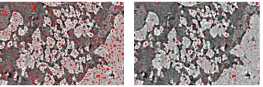
Note that because the min and max functions return binary images, the supremum and infimum in this equation are equivalent to union and intersection respectively. The figure 6 illustrates that the proposed criterion rejects a lot of the gradient minima while marking every pertinent structural component at least once. The zones of influence of the markers are then identified via a watershed
w= watershed(g,m) (12)
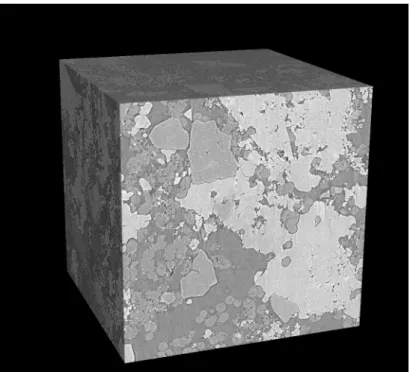
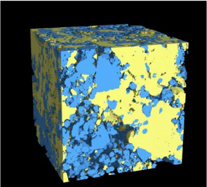
Each zone of influence identified during the watershed process is filled with a constant gray value, computed as the mean value of the image h over this zone. As a result a mosaic of flat zones is obtained which is much simpler than the starting image as illustrated in figure 3. Using the histogram (figure 4, blue curve) the threshold levels are easily identified (as the minimum values between the peaks). On the 2-d zooms (figure 5) one can see that the mosaic filtering improves the quality of the segmentation. Particularly on the ”complex” zone, the spurious silica has disappeared. The very thin details (smaller than the biggest structuring element used during the ASF step) have indeed been lost but the structure at a bigger scale is well preserved. This is a obviously a compromise. The full 3-d results of the segmentation are presented in figures 7 and 8.
which is currently being parallelized. ←insert Fig. 4 ←insert Fig. 5 ←insert Fig. 6 ←insert Fig. 7 ←insert Fig. 8
CONCLUSION
In this contribution an efficient technique enabling to denoise and to segment X-ray tomographic images of a particular multiphasic porous media stone was presented. It relies on two trade-offs. (1) The classical ASF are shown to be efficients but have to be limited in terms of structuring element size in order to preserve the smaller struc-tural components of the image. The small pixel size relatively to the dimensions of the structural components to be preserved allows to bring the ASF up to structuring elements of 3 voxels radius. (2) The mosaic operator is built upon a marker set determined in a pragmatic way. It yields as few flat zones as possible in order to simplify the image enough, while insuring no structural component is missed.
ACKNOWLEDGEMENT
The author would like to thank ´Elodie Boller, Peter Cloetens, and Jos´e Baruchel (ID 19, ESRF,Grenoble) for the scientific support concerning tomography experiments.
Portions of this study were conducted as part of the R´egion Centre/SOLEIL project funded by the R´egion Centre that granted one of us.
REFERENCES
Adler PM (1992). Porous media: geometry and transport. Butterworth-Heinemann. Amoroso GG, Fassina V (1983). Stone decay and conservation. In: Material Science
Monographs 11. Amsterdam: Elsevier.
Anguy Y, Ehrlich R, Ahmadi A, Quintard M (2001). On the ability of a class of random models to portray the structural features of real, observed, porous media in relation to fluid flow. Cement and Concrete Composites 23:313–30.
Appoloni CR, Fernandes CP, Rodrigues CRO (2007). X-ray tomography study of a sandstone reservoir rock. Nulear instruments and methods in physics research A 580:629–32.
Baruchel J, Buffiere JY, Cloetens P, Michiel MD, Ferrie E, Ludwig W, Maire E, Salvo L (2006). Advances in synchrotron radiation microtomography. Scripta Materialia 55:41–6.
Baruchel J, Buffiere JY, Maire E, Merle P, Peix G (2000). X-Ray Tomography in Material Science. Herm`es.
Benouali AH, Froyen L, Dillard T, Forest S, Nguyen F (2005). Investigation on the influence of cell shape anisotropy on the mechanical performance of closed cell aluminium foams using micro-computed tomography. Journal Of Materials Science 40:5801–11.
Betson M, Barker J, Barnes P, Atkinson T (2005). Use of synchrotron tomographic techniques in the assessment of diffusion parameters for solute transport in groundwater flow. Transport in Porous Media 60:217–23.
Betson M, Barker J, Barnes P, Atkinson T, Jupe A (2004). Porosity imaging in porous media using synchrotron tomographic techniques. Transport in porous media 57:203– 14.
Beucher S (1990). Segmentation d’images et morphologie math´ematique. Ph.D. thesis, ´
Ecolde des mines de Paris.
Beucher S (1992). The watershed transformation applied to image segmentation. Scanning Microscopy International 6:299–314.
Beucher S, Lantuejoul C (1979). Use of watersheds in contour detection. In: Proceedings of the internal workshop on image processing. CETT/IRISA.
Beucher S, m. Bilodeau, Yu X (1990). Road segmentation by watershed algorithms. In: Proceedings of the Pro-art vision group. PROMETHEUS workshop.
Brunet-Imbault B (1999). Etude des patines de pierres calcaires mises en oeuvre en´ R´egion Centre. Ph.D. thesis, University of Orl´eans, France.
Camuffo D (1995). Physical weathering of stones. Science of the Total Environment 167:1–14.
Carminati A, Kaestner A, Ippisch O, Koliji A, Lehmann P, Hassanein R, Vontobel P, Lehmann E, Laloui L, Vulliet L, Fl¨uhler H (2006). Water flow between soil aggregates. Transport in Porous Media 68:219–36.
Chung R, kin Ho C (2000). 3-d reconstruction from tomographic data using 2-d active contours. Computers and Biomedical Research 33:186–201.
Cnudde V, Cnudde JP, Dupuis C, Jacobs PJS (2004). X-ray micro-ct used for the localization og water repellents and consolidants inside natural building stones. Materials characterization 53:259–71.
Cnudde V, Jacobs PJS (2003). Monitoring of weathering and conservation of building materials through non-destructive x-ray computed microtomography. Environmental geology 46:477–85.
Dessandier D (1995). ´Etude du milieu poreux et des propri´et´es de transfert des fluides du tuffeau blanc de Touraine. Application `a la durabilit´e des pierres en œuvre. Ph.D. thesis, University of Tours, France.
du Roscoat SR, Bloch JF, Thibault X (2005). Synchrotron radiation microtomography applied to investigation of paper. Journal of Physics D Applied Physics 38:78–84. Dullien FAL (1992). Porous media, fluid transport and pore structure. Academic Press.
Second edition.
Erdogan S, Quiroga P, Fowler D, Saleh H, Livingston R, Garboczi E, Ketcham P, Hagedorn J, Satterfield S (2006). Three-dimensional shape analysis of coarse aggregates: New techniques for and preliminary results on several different coarse aggregates and reference rocks. Cement and Concrete Research 36:1619–27.
Galan E, Carretero M, Mayoral E (1999). A methodology for locating the original quarries used for constructing historical buildings: application to malaga cathedral, spain. Engineering Geology 54:287–98.
structure changes during decomposition of fresh residue: X-ray tomography analyses. Geoderma 34:82–96.
janaki SS, ebenezer D (2006). A blur reducing adaptative filter for the removal of mixed noise in images. Springer Netherlands, 25–9.
Jones AC, Milthorpe B, Averdunk H, Limaye A, Senden TJ, Sakellariou A, Sheppard AP, Sok RM, Knackstedt MA, Brandwood A, Rohner D, Hutmacher DW (2004). Analysis of 3d bone ingrowth into polymer scaffolds via micro-computed tomography imaging. Biomaterials 25:4947–54.
Kaestner A, Schneebeli M, Graf F (2006). Visualizing three-dimensional root networks using computed tomography. Geoderma 136:459–69.
Kak AC, Slaney M (2001). Principles of Computerized Tomographic Imaging. Society for Industrial and Applied Mathematics.
Ketcham RA (2005). Three-dimensional grain fabric measurements using high-resolution x-ray computed tomography. Journal of Structural Geology 27:1217–28.
Lambert J, Cantat I, Delannay R, Renault A, Graner F, Glazier JA, Veretennikov I, Cloetens P (2005). Extraction of relevant physical parameters from 3d images of foams obtained by x-ray tomography. Colloids and Surfaces A Physicochemical and Engineering Aspects 263:295–302.
Lindquist WB, Venkatarangan A (1999). Investigating 3d geometry of porous media from high resolution images. Physics and Chemistry of the Earth Part A Solid Earth and Geodesy 25:593–9.
Maire E, Colombo P, Adrien J, Babout L, Biasetto L (2007). Characterization of the morphology of cellular ceramics by 3d image processing of x-ray tomography. Journal of the European Ceramic Society 27:1973–81.
Maksimovic R, Stankovic S, Milovanovic D (2000). Computed tomography image analyzer: 3d reconstruction and segmentation applying active contour models – ’snakes’. International Journal of Medical Informatics 58–59:29–37.
for porosity measurement. Journal of Materials Processing Technology 192–193:391– 6.
Maravelaki-Kalaitzaki P, Bertoncello R, Biscontin G (2002). Evaluation of the initial weathering rate of istria stone exposed to rain action, in venice, with x-ray photoelectron spectroscopy. Journal of Cultural Heritage 3:273–82.
Matheron G (1975). Random sets and integral geometry. New York: Wiley.
Mendoza F, Verboven P, Mebatsion HK, Kerckhofs G, Wevers M, Nicola¨ı B (2007). Three-dimensional pore space quantification of apple tissue using x-ray computed microtomography. Planta 226:559–70.
Prodanovi´c M, Lindquist W, Seright R (2005). Porous structure and fluid partitioning in polyethylene cores from 3d x-ray microtomographic imaging. Journal of Colloid and Interface Science 298:282–97.
Qatarneh SM, Crafoord J, Kramer EL, Maguire GQ, Brahme A, Noz ME, Hy¨odynmaa S (2001). A whole body atlas for segmentation and delineation of organs for radiation therapy planning. Nuclear Instruments and Methods in Physics Research Section A Accelerators Spectrometers Detectors and Associated Equipment 471:160–4.
Ramlau R, Ring W (2007). A mumford-shah level-set approach for the inversion and segmentation of x-ray tomography data. Journal of Computational Physics 221:539– 57.
Rozenbaum O, Le Trong E, Rouet JL, Bruand A (2007). 2d-image analysis: A complementary tool for characterizing quarry and weathered building limestones. Journal of Cultural Heritage 8:151–9.
Salvo L, Cloetens P, Maire E, Zabler S, Blandin JJ, Buffi`ere JY, Ludwig W, Boller E, Bellet D, Josserond C (2003). X-ray micro-tomography an attractive characterisation technique in materials science. Nuclear Instruments and Methods in Physics Research Section B Beam Interactions with Materials and Atoms 200:273–86.
Serra J (1982). Image analysis and mathematical morphology. London: AcademicPress. Serra J (1988). Image analysis and mathematical morphology, vol. 2: theoretical
advances. London: AcademicPress.
Sezgin M, Sankur B (2004). Survey over image thresholding techniques and quantitative performance evaluation. Journal of Electronic Imaging 13:146–68.
Sheppard AP, Sok RM, Averdunk H (2004). Techniques for image enhancement and segmentation of tomographic images of porous materials. Physica A 339:145–51. Tiano P, Cantisani E, Sutherland I, Paget J (2006). Biomediated reinforcement of
weathered calcareous stones. Journal of Cultural Heritage 7:49–55.
Torraca G (1976). Treatment of stone monuments: a review of principles and processes. Conservation Stone 1:297–315.
T¨or¨ok A (2002). Oolitic limestone in a polluted atmospheric environment in budapest: weathering phenomena and alterations in physical properties. In: Natural stone, weathering phenomena, conservation strategies and case studies. Geological society of London, 363–79.
Vachier C, Meyer F (2005). The viscous watershed transform. Journal of Mathematical Imaging and Vision 22:251–67.
Videla A, Lin C, Miller J (2007). 3d characterization of individual multiphase particles in packed particle beds by x-ray microtomography (xmt). International Journal of Mineral Processing 84:321–6.
Vincent L, Soille P (1991). Watersheds in digital spaces: an efficient algorithm based on immersion simulations. IEEE Transactions on Pattern Analysis and Machine intelligence 13:583–98.
50 µm
(a)
(b)
(c)
Fig. 1: SEM image of a tuffeau sample with (a) sparitic calcite (large grains), (b) micritic
200 µm (a) (c) (d) (e) (f) (b)
Fig. 2: One slice extracted from a 3-d tomographic image of a tuffeau sample. The image
is 2048× 2048 pixels, pixel size is 0.28µm (the radius of the sample is≈600µm) with (a) resin, (b) silica (opal sphere), (c) air bubble in the resin (caused by the impregnation process), (d) silica (quartz crystal), (e) calcite and (f) phyllosilicate. The rectangle marks the location of the zoomed image that appears in figure 3-(a).
0 50 100 150 200 250 500 550 600 650 700 750 800 (a) 0 50 100 150 200 250 500 550 600 650 700 750 800 (b) 0 50 100 150 200 250 500 550 600 650 700 750 800 (c) 0 50 100 150 200 250 500 550 600 650 700 750 800 (d) 0 50 100 150 200 250 500 550 600 650 700 750 800 (e)
Fig. 3: Illustration of the image processing. In the left column a 2-d zoom in the sample (white rectangle in figure 2) undergoes the image treatment. The images are
300× 200 pixels with pixel size 0.28µm. In the right column, a line of the zoomed image
(noted in red in the left column) is plotted (pixel coordinate in abscissa, gray level in ordinate). From top to bottom: (a) the original image; (b) after step 1 of the ASF; (c) after step 2, (d) after step 3, (e) after the mosaic operator. The histograms of the whole 3-d image at each steps are visible on figure 4.
0 5e+06 1e+07 1.5e+07 2e+07 2.5e+07 3e+07 0 50 100 150 200 250 Original ASF Mosaic
Fig. 4: Evolution of the histogram of a 1024× 1024 × 1024 voxels image during the
image processing. The starting image is visible on figure 7. Original is the histogram of the original images (figure 3-(a)), ASF after the ASF (figure 3-(d)) and Mosaic after the watershed (figure 3-(e)).
Fig. 5: Illustration of the segmentation. Left column: a 2-d zoom (300× 200 pixels) of a
”simple” zone. Right column a zoom (same size) of a ”complex” zone, containing micritic calcite. First row: unfiltered gray-level images. Second row: segmentation results after the ASF step (black: resin, blue: silica, yellow: calcite). Third row: segmentation result after the mosaic step.
Fig. 6: Illustration of the marker used for the mosaic. Left: minima of the gradient of the
ASF filtered image in red superimposed over the original raw image. Right: the marker actually used to build the mosaic.
Fig. 7: 3-d illustration of the segmentation process: original image. The image is 1024×
Fig. 8: 3-d illustration of the segmentation process: segmented version of the image in