An approach to predict operational performance of airline schedules using aircraft assignment key performance indicators

An Approach to Predict Operational Performance

of Airline Schedules Using Aircraft Assignment

Key Performance Indicators

by

Robin Riedel

Submitted to the Department of Aeronautics and Astronautics in partial fulfillment of the requirements for the degree of

Master of Science in Aeronautics and Astronautics

at the

MASSACHUSETTS INSTITUTE OF TECHNOLOGY

June 2006

All rights reserved.

@

Massachusetts Institute of Technology 2006.

A uthor ...

Department of Aeronautics and Astronautics

May 22nd, 2006

Certified by ... _., . .. . . ...--. - --. ...i ...- -. - - - --. .7

John-Paul B. Clarke

Principal Research Scientist Thesis

Supervisor

I

Accepted by ...

Jaime Peraire Professor of Aeronautics and Astronautics

An Approach to Predict Operational Performance of Airline

Schedules Using Aircraft Assignment Key Performance

Indicators

by

Robin Riedel

Submitted to the Department of Aeronautics and Astronautics on May 22nd, 2006, in partial fulfillment of the

requirements for the degree of

Master of Science in Aeronautics and Astronautics

Abstract

This thesis presents an approach for predicting operational performance of airlines on the basis of flight schedules and aircraft assignments. The methodology uses aggregate measures of properties of aircraft assignments, called Aircraft Assignment Key Performance Indicators (KPIs), and aims to find correlations between them and the operational performance of the airline. A simulation experiment is prepared to gather a large set of data points for analysis. A motivation is given for the use of control theoretic approaches in airline operations to utilize the KPIs as a basis for initial planning and corrective actions.

Thesis Supervisor: John-Paul B. Clarke Title: Principal Research Scientist

Acknowledgments

There are a number of people who contributed to this work. I would like to express my gratitude to

- my parents, grandparents and siblings for their support over the years I spent at MIT.

- my thesis advisor, John-Paul Clarke, as well as all other participants in the Airline KPI Project, especially Michel Turcotte at Air Canada, Erik Ander-sson, Fredrik JohanAnder-sson, Stefan Karisch, and Antonio Viegas Alves at Car-men Systems, Gerrit Klempert, Christoph Klingenberg, Michael Mederer and Brigitte Stolz at Lufthansa, and Terran Melconian, Praveen Pamidimukkala, and Michelangelo Raimondi at MIT, for the productive and pleasant collabora-tion.

- my friends and colleagues at MIT, especially Louis Breger, Nayden Kambouchev,

Georg Theis, and Laura Waller for their continuous support in preparing this thesis.

- Cynthia Bernhart, David Darmofal, Amedeo Odoni, Jaime Peraire, Raul Radovitzky,

and David Robertson at MIT for their exceptional teaching and their integrity, that made my time at MIT that much more enjoyable.

- Christian Kaufer for his continuous support of my flying career which I could not have continued throughout graduate school otherwise.

Contents

1 Introduction 13

1.1 M otivation . . . . 13

1.2 T hesis O utline . . . . 15

2 Overview of Airline Scheduling, Operation, and Recovery 17 2.1 Airline Scheduling . . . . 17 2.1.1 Flight Scheduling . . . . 18 2.1.2 Aircraft Assignment . . . . 20 2.1.3 Crew Scheduling . . . . 22 2.2 Airline Operation . . . . 23 2.3 Airline Recovery . . . . 27

3 Key Performance Indicators and Output Measures 29 3.1 General Definitions . . . . 29

3.2 Aircraft Assignment Related Key Performance Indicators . . . . 31

3.2.1 Fleet Assignment Buffer Statistics . . . . 31

3.2.2 Global Fleet Composition Indicators . . . . 35

3.2.3 Swap Option Indicators . . . . 39

3.3 Output Measures . . . . 42

3.3.1 Delay Minutes . . . . 43

3.3.2 On-Time Performance . . . . 44

4.1 B ackground . . . .

4.2 Example of an Application of Control Theory in Airline Operations .

5 Simulation Setup

5.1 MIT Extensible Air Network Simulation

5.2 Integrated Operations Control System 5.3 Simulation Input . . . .

5.3.1 Flight Schedules . . . .

5.3.2 Aircraft Assignments . . . .

5.3.3 Taxi Times . . . .

5.3.4 Flight Times . . . .

5.3.5 Airport Capacity Profiles . . . . .

5.3.6 Weather Scenarios . . . .

5.3.7 Airport Traffic . . . .

6 Proposed Analysis

6.1 Initial A nalysis . . . .

6.2 Optimization of Weighting Coefficients and Functions . . . .

7 Directions for Future Research A Acronyms and Initialisms

B Derivation of Probability Density Function of Flight Time C Weather Scenarios 47 49 57 . . . . 57 . . . . 59 . . . . 60 . . . . 60 . . . . 60 . . . . 61 . . . . 63 . . . . 67 . . . . 69 . . . . 69 73 73 74 77 81 83 85

List of Figures

2-1 Parts of an Airline Schedule . . . . 17

2-2 Time Terminology . . . . 18

2-3 Network Strategies . . . . 19

2-4 Example of Delay Propagation . . . . 24

2-5 On-Time Performance and Delay Causes by Number of Operations in October 2005 (USA only) . . . . 25

2-6 Delay Causes by Delay Minutes in October 2005 (USA only) . . . . . 25

2-7 Original Delay Causes by Delay Minutes in October 2005 (USA only) 26 3-1 Temporal Relation of KPIs and the performance . . . . 30

3-2 Timeline of the Ground Process Between Two Flights . . . . 32

3-3 Example Buffer Weighting Functions . . . . 34

3-4 Timeline of Aircraft Arrivals and Departures . . . . 35

3-5 GFCI exam ples . . . . 37

3-6 Influence of Choice of Wf on GFCI . . . . 38

3-7 Timeline of Ground Arcs of Aircraft of Different Fleet Types . . . . . 42

3-8 Example On-Blocks Delay Distribution and On-Time Performance . . 45

4-1 Control System Block Diagrams . . . . 48

4-2 Airline Delay Control System . . . . 51

4-3 Response of the P-controlled System to a Change in DMPAdesired . . 52

4-4 Response of the System for Different Gain Values . . . . 53

4-5 Response of the System to Constant Weather . . . . 54

5-1 MEANS Modular Structure ... ... 58

5-2 Taxi Time Distributions . . . . 62

5-3 Example Flight Time Distributions . . . . 64

5-4 Example Unimpeded Flight Time Distributions . . . . 65

5-5 Airport Capacity Profiles . . . . 68

5-6 A irport Traffic . . . . 71

List of Tables

2.1 Example Overview of an Airline's Maintenance System [3] . . . . 22

3.1 _{Properties of Aircraft for Example Airline . . . . 38}

Chapter 1

Introduction

1.1

Motivation

Delays are an expected part of air travel today. Over the last seven years, approxi-mately one fifth (21.5%) of all domestic flights in the United States of America (USA) were either delayed' or canceled [22]. The situation in Europe is similar [11]. A study estimates that flight delays in scheduled European air traffic in 1999 cost airlines between EUR3.0 and EUR5.1 billion [9]. With the recent strengthening of passenger rights in the European Union [24, 20], the cost to airlines is likely to increase further. One possible way to reduce delays during operation is to design robust airline schedules [4]. By rearranging existing and adding additional reserves or buffers into a schedule, delays can be reduced and their propagation can be limited. However, a tradeoff exists between cost efficiency and robustness. While the cost impact of adjust-ments to improve robustness is easily determined from the schedules and accounting data, the operational improvements are difficult to estimate. As a result, reactive approaches, i.e., airline recovery, are more common than proactive approaches, i.e., robust scheduling. It is relatively easy for the mid-level decision maker to justify costs created by bad weather. It is much harder to justify costs for proactive adjustments that will reduce costs in the case of bad weather in the future. This is especially true

1_{A delayed flight in this statistic is defined as a flight that arrives at the arrival gate 15 minutes}

because it is usually uncertain how well the proactive measures will reduce costs on a bad weather day.

To reduce delays through robust scheduling, an understanding of the effects of possible airline schedule adjustments on the airline operation is required. An airline needs to be able to predict the performance of its schedule in order to make successful adjustments. Such predictions can be based on past performance, if the environment and the parameters of the operation remain similar. In fact, a structured analysis of the relationship between scheduling factors and operational performance should provide insight into the operation and assist with future predictions.

However, airline operations are complex. The airlines within the Lufthansa Cor-poration2, for example, operate more than 1500 flights on a typical day transporting 128,000 passengers [3]. Not only does the airline schedule vary, but there are also varying uncontrollable external factors that influence the operation, such as weather conditions. Thus, variations exist and no day of operation is like another. Therefore, it is extremely unlikely that a large set of identical schedules in different weather con-ditions or different schedules in identical weather concon-ditions would exist in historic data. Such sets are, however, required to conduct structured factor analysis to iden-tify what properties of a schedule make it more robust to the uncertain conditions in which the schedule is operated in.

In this thesis, a simulation platform is developed for creating such a data set, an approach to analyze aircraft assignment measures and their correlation to operational performance is presented, and a set of simulation input data is described. In the proposed approach, the airline operation is simulated using an air network simulation and an airline recovery tool and multiple schedules are examined over a range of different weather scenarios to provide a level of granularity of data points that is unavailable in historic data. Multiple Leading Key Performance Indicators (LKPIs) aggregating information on the aircraft routing are presented and an analysis of their correlation to operational performance measured by output measures is suggested. Also, a view on airline operations, based on control theory, is introduced as a potential

2

framework for utilizing the LKPIs examined in the analysis.

1.2

Thesis Outline

This thesis is divided into the following chapters:

In Chapter 2 an overview of airline processes is provided. This includes the airline scheduling, operation, and recovery processes.

In Chapter 3 a general definition of the term Key Performance Indicator and definitions and examples of the Leading Key Performance Indicators and output mea-sures that should be examined in the analysis are presented.

In Chapter 4 an alternate view of airline processes is introduced. This view is based on control theory and is intended to provide a framework for the use of Key Performance Indicators in airline scheduling and recovery.

In Chapter 5 the simulation platform and inputs are presented. This includes a description of the MIT Extensible Air Network Simulation (MEANS), the Inte-grated Operations Control System (IOCS), the simulation environment, and detailed information about the benchmark simulation inputs.

In Chapter 6 the proposed analysis for determining the correlations between the Leading Key Performance Indicators and output measures based on the simulation results is presented.

In Chapter 7 shortcomings of simulation environment and the proposed anal-ysis are identified and suggestions are made for for further research leading to the application of the approach.

Chapter 2

Overview of Airline Scheduling,

Operation, and Recovery

2.1

Airline Scheduling

An airline typically plans its operation ahead of time in an airline schedule. Generally, the airline schedule consists of three major parts: a) the flight schedule, b) the aircraft assignment and c) the crew schedule (Figure 2-1).

1~

Airline Schedule

Flight Schedule

Aircraft Assignment

L

Fleet Assignment Aircraft Routing

J

Crew Schedule

Crew Pairings C Crew Roster J

2.1.1

Flight Scheduling

The basic "building block of a flight schedule is the flight leg. A flight leg is defined by a departure airport and time and an arrival airport and time. For the departure and arrival times there exist two different time references, shown in Figure 2-2: block time and flight time.

off-blocks take-off landing on-blocks

taxi-out time flight time taxi-in time

block time

Figure 2-2: Time Terminology

Block time is the time between departure from the gate at the departure airport (off-blocks) and arrival at the gate at the arrival (on-blocks). The terms off- and on-blocks refer to blocks (or chocks) that are put in front of and behind the aircraft wheels on the ground to stop the aircraft from moving. The exact definition of the beginning and ending of block time varies. Often, off-blocks is defined as the time at which the aircraft begins to move on the ground and on-blocks as the time at which the aircraft comes to a complete stop at the final parking position on the ground. In some cases, off- and on-blocks times are defined in relation to the engine state, where off-blocks will be the time at which the first engine is started (which does not necessarily have to be prior to aircraft movement, e.g., in the case of a push back at the gate) and on-blocks will be the time at which the last engine is shut down. Flight time is the time between take-off (at which the aircraft leaves the ground and goes airborne) and landing.

A flight schedule is a list of flight legs. The design of a flight schedule is based on numerous factors, among which are market demands, expected revenues and costs, crew constraints, aircraft availability and performance, minimum ground times, legal

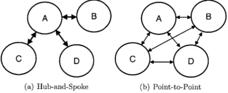
constraints, route restrictions, overall airline strategy, competitor behavior, and air-line alliances. In the creation of flight schedules, the airair-line network strategy plays an important role.

A B A B

C _D

C _D

(a) Hub-and-Spoke (b) Point-to-Point

Figure 2-3: Network Strategies

For example, consider a typical hub-and-spoke network as shown in Figure 2-3(a). Airport A serves as a hub and passengers who want to travel from one spoke (airports B, C, or D) to another spoke have to connect through the hub. An alternative network strategy is that of the point-to-point network shown in Figure 2-3(b), where all airports are connected by direct flights. In the hub-and-spoke case the airline operates only three different routes compared to the point-to-point case where it operates six routes. Given the same availability of resources, the flight frequency in the hub-and-spoke network is higher than in the point-to-point network. The thickness of the flight connection arrows between the airports in Figure 2-3 indicates the number of flights per days. Large carriers usually operate a mixed network of both hub-and-spoke and point-to-point flights, where the hub-and-spoke portion is dominant. To provide service between different spokes, the flight schedule has to be created in such a way as to enable passengers to connect between flights. This results in banks at the hub in the schedule during which connections between important spokes are available.

For most major scheduled airlines, flight schedules are set and published multiple months before the day of operation. Although major scheduled airlines operate the majority of flight legs daily, some variation in flight schedules between different days exists. These variations could be, for example, driven by passenger demand or aircraft

availability. As a result, the flight schedules for any two days will almost never be identical.

2.1.2

Aircraft Assignment

During aircraft assignment, a specific aircraft is assigned to each of the flight legs in the flight schedule. Often, aircraft assignment is broken down into two sequential parts: fleet assignment and aircraft routing. The reason for this separation is that the required computing power is reduced significantly and that the fleet assignment can be created earlier because the required input data for the fleet assignment problem is available earlier than the required input data for the overall aircraft assignment problem. The fleet assignment process only requires aggregate aircraft availability and maintenance requirements which are available much earlier than detailed air-craft availability and maintenance requirements. As a result, fleet assignment can be carried out soon after flight schedule design.

The fleet assignment for a flight schedule assigns each flight leg in the schedule to a specific fleet. A fleet is a group of aircraft with a common property. Often, that common property is aircraft type (e.g., the Boing 747 fleet or the Airbus A300 fleet), stage length (e.g., long haul fleet and short haul fleet), or crew requirement (e.g., the Boeing 757 and 767 fleet can be operated by the same pilots). Fleets can be broken down into subfleets (e.g., the Airbus A320 series fleet could include the Airbus A320 and the Airbus A321 subfleets).

The modern fleet assignment process for large airlines utilizes mathematical pro-gramming methods to optimize an objective function (usually expected profits). This optimization is restricted by a number of constraints: Cover constraints require that each flight leg will be assigned to exactly one fleet. Balance constraints ensure that aircraft departing an airport have arrived at that airport before and have had at least the minimum ground time on the ground at the airport. Fleet size constraints ensure that the number of aircraft required in the assignment does not exceed the size of the available fleet. Additional operational constraints (e.g., minimum ground times for aircraft turnarounds or noise restrictions at airports prohibiting certain fleets to

operate there) may also need to be satisfied. The minimum ground time (MinGT) for an aircraft at an airport between two flights is the minimum time required between on-blocks of one flight and off-blocks of the next flights to prepare the aircraft for the next departure (a process also called turnaround). During the turnaround the aircraft is unloaded, refueled, serviced (e.g., cleaned and catered) and loaded again. MinGT depends on multiple factors, among which are airport, number of passengers and cargo, aircraft type (e.g., size, break cooling time) and services provided (e.g., catering, cleaning, fuel). The first published modern fleet assignment method was developed by Abara in 1989 [2] and many extensions and reformulations exist today.

During the aircraft routing (or aircraft maintenance routing) process, a specific aircraft (or tailnumber) of a given fleet type is assigned to each of the flight legs that was assigned to the fleet during the fleet assignment process. In addition to satisfying cover, balance and fleet size constraints, as in the fleet assignment, the maintenance routing also has to provide maintenance feasibility. Aircraft need to undergo routine maintenance checks prescribed by the airline's maintenance manual, which needs to be approved by the competent authority. These checks are usually time-based (e.g., daily or weekly checks), flight-time-based (e.g., 500 hour check) or cycle-based (5,000 cycle check). While time-based check requirements are known well ahead of time, the due dates for flight-time-based and cycle-based maintenance depend on the usage of the aircraft and, therefore, cannot be scheduled many months ahead. For example, the maintenance system of Lufthansa is shown in Table 2.1.As can be seen, some variability exists in both the intervals and ground times per event. More precise estimates of the values within these ranges become available as the time of the event draws near.

In addition to routine maintenance, aircraft will also need to undergo non-routine maintenance. Non-routine maintenance includes the repair of technical failures and the implementation of Airworthiness Directives issued by the authorities or service bulletins issued by the manufacturer. Non-routine maintenance requirements are usually not known well ahead of time. Due to this limited availability of maintenance information ahead of time, the aircraft maintenance routing is usually done a few

Table 2.1: Example Overview of an Airline's Maintenance System

[3]

Event Interval Ground Time Work Hours

per Event per Event

Pre-Flight-Check before every flight 30-60 minutes 1

Ramp-Check daily 2 - 5 hours 6-35

Service-Check weekly 2.5 - 5 hours 10-55

A-Check ca. 350 - 650 flight hours 5 - 10 hours 45-260

B-Check ca. 5 months 10 - 28 hours 150-700

C-Check 15 - 18 months 36 - 48 hours 650-1,800

IL-Check 5 - 6 years ca. 2 weeks up to 25,000

D-Check 5 - 10 years ca. 4 weeks up to 60,000

weeks before the day of operation.

2.1.3

Crew Scheduling

The crew schedule for a flight schedule is the assignment of crew members to flight legs. A typical crew for a passenger airline flight consists of a flight-deck (or cockpit) crew and a cabin crew. The flight-deck crew usually consists of a Captain (or Commander, Pilot in Command) and a First Officer (or Copilot, Second in Command). The cabin crew usually consists of a Purser (or Chief Flight Attendant, Chef de Cabin) and one or more Flight Attendants (or Cabin Attendants). Depending on aircraft type and purpose of flight, additional crew members such as a flight engineer, a load master, a translator or long range relief crew may be required.

The modern crew scheduling process consists of two phases: creation of a) crew pairings and b) crew rosters. A crew pairing is a list of flight legs that can be operated by a single crew member. A crew roster is the assignment of individuals to these pairings. In the creation of both crew pairings and rosters, multiple constraints need to be considered, among which are cover constraints, balance constraints, crew availability constraints, crew qualification and training requirements, legal constraints (e.g., maximum duty time rules), and labor agreements. Crew scheduling is usually carried out three to six weeks before the day of operation.

2.2

Airline Operation

Generally, the goal of airline operation is to execute the airline schedule with minimum costs and maximum passenger satisfaction. Airline operation is cost-driven; very few revenues can be raised within the operations domain of an airline since, by the time of operation, tickets have already been sold.

Execution of an airline schedule is complicated by the fact that assumptions made during the scheduling process are not always valid. There exists a wide range of influences that cannot be controlled, or even accurately predicted, by the airline. These influences include meteorological conditions, other air traffic (e.g., flights by other airlines, the military, and general aviation), Air Traffic Control (ATC) actions, equipment failures, and crew member absenteeism. They have the potential to cause significant differences between the environment for which the airline schedule was designed and the environment in which that schedule must be implemented. This change of environment can cause the airline schedule to become infeasible.

A disruption in an airline operation is an event that causes infeasibilities in the future of the airline schedule. For example, consider a snow storm at an airport which will require aircraft to de-ice before the flight. As a result, the time between off-blocks and take-off of the aircraft will be increased. Assuming that the off-blocks departure cannot be made earlier (since passengers will arrive for the scheduled off-blocks departure time) the take-off is also delayed and a disruption occurs. If the aircraft can compensate for the delay en route (by reducing the actual flight time) and land at the scheduled time, the disruption will have been recovered. However, if this is not possible, the resulting arrival delay may cause more infeasibilities in the airline's schedule (e.g., delay propagation to other flights) or in passenger travel plans (e.g., missed connection flights).

Arrival delays often cause schedule infeasibilities through delay propagation to other flights. Delay propagation to other flights occurs when an aircraft or crew arrives at a destination behind schedule and is scheduled for another flight which it can no longer serve at the scheduled time. As a result, the next flight of the aircraft

and/or crew will be delayed until the aircraft or crew are ready. This kind of delay is called propagated delay or reactionary delay [11]. For example, consider the timeline for a specific aircraft shown in Figure 2-4. The top row represents the schedule and the bottom row represents the actual events for the aircraft. The horizontal axis represents time. A disruption in time occurs during taxi out of flight 111 and the take-off of the flight is delayed. The delay propagates through to the next flight of the aircraft, flight 112, since the delay cannot be recovered during flight 111 (by flying or taxing faster) or on the ground between flight 111 and 112 (because the scheduled ground time is equal to MinGT).

scheduled ₁₁₁

-- ₁₁₂₂

actual 111 112 time

original delay minimum ground time

Figure 2-4: Example of Delay Propagation

Frequently, disruptions will span across resource boundaries such that a single disruption can have a negative impact on multiple resources. If, for example, a flight arrives delayed, both the aircraft and the crew are delayed. If the crew is scheduled to fly on other aircraft following the delayed flight, at least two additional flights could be delayed as a result: the next flight of the aircraft and the next flight of the crew

(or even more flights if the crew does not stay together).

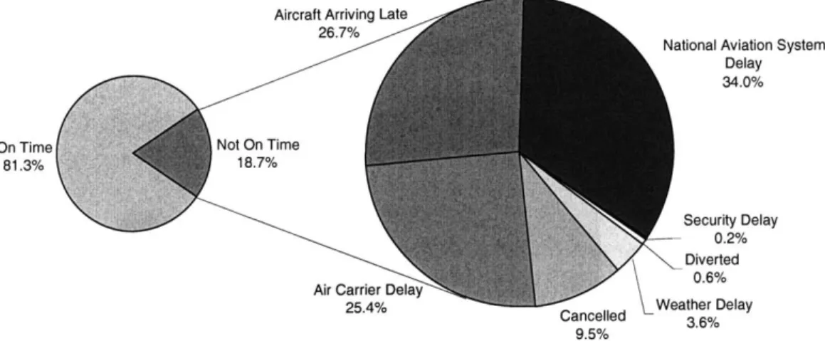
In the USA, approximately one quarter of all delayed flights (or about 4.5% of all flights operated) are delayed due to delay propagation to other flights (aircraft arriving late), where a delayed flight in this statistic is defined as a flight that arrives 15 or more minutes after its scheduled arrival time [22]. An overview of the causes of flight delays in the USA in October 2005 is given in Figure 2-5.

The distribution of causes for flight delays by delay minutes is shown in Figure

2-6. There are three major causes for flight delays: weather (5.8% + 33.9% * 76.6% =

31.8%), propagation delay (32.5%) and air carrier delay (27.6%).

For every propagated delay there must be an original cause, i.e., the cause for the first delay in a propagation sequence. The portion of propagation delay in Figure

Aircraft Arriving Late 26.7%

Not On Time 18.7%

Air Carrier Delay 25.4%

Cancelled

9.5%

National Aviation System Delay 34.0% Security Delay 0.2% Diverted 0.6% Weather Delay 3.6%

Figure 2-5: On-Time Performance and Delay Causes by Number of Operations in October 2005 (USA only)

Weather 76.6%

Aircraft Arriving Late

Security Delay 0.2% Weather Delay

5.8%

Air Carrier Delay 27.6% National Aviation System Delay 33.9% Closed Runway 6.6% Other 2.7% Equipment 3.3% LVolume 10.8%

Figure 2-6: Delay Causes by Delay Minutes in October 2005 (USA only)

On Time

2-5 can be assigned to these original causes. If it is assumed that the distribution of original causes for the propagation delays is equal to the distribution of causes shown in Figure 2-6, excluding the portion due to aircraft arriving late, a distribution of original delay causes (shown in Figure 2-7) can be derived. Approximately half of

Other

12.0%

Weather Caused Delay

49.5%

Air Carrier Delay

38.5%

Figure 2-7: Original Delay Causes by Delay Minutes in October 2005 (USA only)

all delays in the USA are originally caused by weather (see Figure 2-7). Within this group of weather causes, there exist two subgroups depending on where the weather occurs. En route weather is weather that the aircraft encounters during the flight between airports. Examples of unfavorable en route weather are strong turbulence or hurricanes. They may require the pilot to take a less direct flight path, which may result in a longer flight time. Also, if certain sectors of the airspace become unusable due to en route weather, the remaining sectors will be utilized more which may lead to capacity bottlenecks and ATC driven delays. Airport weather affects departing and arriving traffic flows to that airport. When the weather at an airport becomes unfavorable it can either slow down certain segments of the flight process for individual aircraft (e.g., freezing rain that requires aircraft to de-ice) or reduce the capacity of the airport as a whole (e.g., heavy crosswinds that make runways unusable). In the latter case, the departing and arriving flows at the airport are affected as a whole. For example, Boston's Logan airport (BOS) operates on three runways in favorable weather conditions, however can be restricted to the usage of only one runway in the case of strong North-Westerly winds. The reduction of capacity in this case might be

as great as 50%, from approximately 120 operations per hour in favorable weather to as few as 60 operations per hour in poor weather [6].

In addition to the airline schedule, passenger travel plans may also become in-feasible due to disruptions. If a passenger travels only on a single delayed flight leg, the passenger will also be delayed. if a passenger travels on an itinerary of multiple flights and needs to connect between flights, a delayed flight could cause the passenger to miss his or her connection and his or her itinerary will not be feasible any more. Missed connections are especially frequent in hub-and-spoke operations, because they rely on passengers to connect between flights.

2.3

Airline Recovery

Airline recovery is the management of disruptions. The goal here is to restore airline schedule feasibility while keeping costs and negative impact on customers low. To achieve this goal, airlines adjust their schedules. Common adjustments are intentional delaying of flight departures, swapping of aircraft, ferrying of aircraft (relocating an aircraft with a non-revenue flight), cancelation of flights, activation of reserve aircraft or crew, and rescheduling of aircraft or crew.

Due to complexity of the airline schedules and constraints on computing power, a general approach is to first attempt recovery within a single resource domain. For example, when a crew disruption occurs, the airline will try to recover this disruption within the crew domain without changing the aircraft routing or flight schedule. If a satisfactory solution cannot be found within a single resource domain, other resources will be included in the recovery. Today, this usually occurs sequentially: A change will be made in one resource domain and then the other resource domains are adjusted to the change sequentially. For example, a change could be made to the flight schedule and then the aircraft schedule and finally the crew schedules will be adjusted to this change.

If passenger travel plans become infeasible due to disruptions, airlines also need to recover their passengers. Common actions by the airlines are rebooking the passenger

onto another flight or itinerary (with the same or a different airline) and compensating the passenger for the disruption of their travel plans (e.g., through restaurant and hotel vouchers).

While recovery personnel and systems today understand a wide range of correla-tions between different resource domains, state-of-the-art recovery is rarely globally optimal due to the sequential approach. Multiple airlines and decision support soft-ware developers are developing a new generation of integrated recovery tools that will find a global optimum over multiple domains, including aircraft, crew and passengers.

Chapter 3

Key Performance Indicators and

Output Measures

3.1

General Definitions

The term Key Performance Indicator (KPI) is used in a variety of contexts. It is

commonly used within the business administration context

[191,

where it typically

describes "a significant measure used on its own, or in combination with other key performance indicators, to monitor how well a business is achieving its quantifiable objective" [28]. Other areas in which the term KPI is used include product optimiza-tion [25], educaoptimiza-tion [10, 21, 32] and public administraoptimiza-tion [12, 13]. KPIs are frequently used to benchmark a business against its competitors or its own past performance [19].

An indicator can be defined as "that which serves to indicate or give a suggestion of something; an indication of" [26]. An indication can be defined as "a hint, sugges-tion, or piece of information from which more may be inferred" [26]. Following this definition of an indicator, we define the term Key Performance Indicator as a metric used to indicate or estimate one or more critical success factors of an operation, where this operation is the airline operation, defined as the operation of aircraft to transport passengers between airports of their choice at the time of their choice.

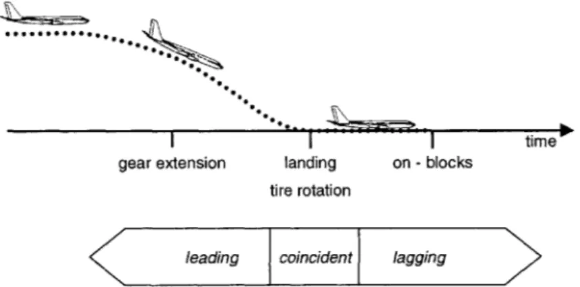
three types of KPIs: lagging, coincident, and leading KPIs. The time difference between KPIs and the performance they indicate is called lead time or lag time. Lagging KPIs trail behind the measure. For example, consider the landing time of an aircraft as the performance (Figure 3-1). A lagging indicator for the landing time could be the on-blocks time. Knowledge of the on-blocks time provides information about the landing time, because both are related through the taxi time. However, the on-blocks time lags the landing time and, therefore, has no predictive value.

time gear extension landing on - blocks

tire rotation

leading coincident lagging

Figure 3-1: Temporal Relation of KPIs and the performance

Coincident KPIs occur concurrently with the performance. In the example above, the time at which the tires of the aircraft rotate for the first time since take-off is a coincident indicator for the landing time; they occur simultaneously, because the tires start rotating when they touch the ground. Leading KPIs change before the performance, giving them predictive value. In the example above, the extension of the landing gear is a leading indicator of the landing time, because the landing gear must be extended before landing. Knowing that the landing gear is usually extended a few minutes before the landing, the gear extension time can be used as a leading indicator (i.e., predictor) for the landing time.

3.2

Aircraft Assignment Related Key Performance

Indicators

The flight schedules and aircraft assignments have a great influence on the opera-tional performance of the airline (see Chapter 2). Therefore, the properties of the flight schedules and aircraft assignments are expected to have predictive value for the operational performance. The following KPIs, based on flight schedules and air-craft assignment, are suggested for further analysis of their correlation with output measures.

3.2.1

Fleet Assignment Buffer Statistics

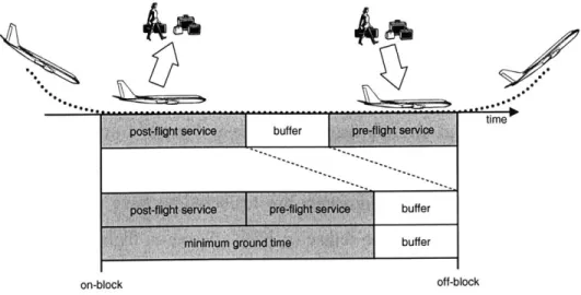
The number of buffers within an airline schedule influences the airline's ability to recover from disruptions. A buffer, in the context of fleet assignment, is extra (or slack) time between the arrival and the departure of an aircraft during which the aircraft is idle. A timeline for an aircraft on the ground between two flights is shown in Figure 3-2. When an aircraft arrives, a post-flight service (e.g., disembarkment, unloading) is conducted at the airport. Before the aircraft departs again, a pre-flight service (e.g., embarkment, loading, refueling) is conducted. The sum of the time required for both post- and pre-flight service is the MinGT (see Section 2.2). While the post-flight service can be conducted without any knowledge of the next flight of the aircraft, the pre-flight service requires this information. It must be known where the aircraft will fly next to determine the required fuel and catering to be loaded.

In the actual operation, buffers exist in between post- and pre-flight service. How-ever, an abstraction can be made by shifting the buffer, as shown in the lower part of Figure 3-2. For this abstraction to hold it must be assumed that the next flight of an aircraft is known early enough for the pre-flight service to be performed. Here we assume that this abstraction holds and we define a buffer as the time span between the arrival of an aircraft plus the minimum ground time of that aircraft at the airport and the next departure of the aircraft. A buffer can be expressed as < a,

f,

t, d >,

post-flight Service -buff er pre flight serviocim

post-flIght service pre-flight se c buffer

minimum ground tim buff er

on-block off-block

Figure 3-2: Timeline of the Ground Process Between Two Flights

where a is the airport at which the buffer occurs, t is the time at which it begins, d is its duration, and

f

is the fleet type of the aircraft.

To obtain the set of buffers from an airline schedule, the set of all aircraft ground arcs (i.e., the period when the aircraft is on the ground) is created from the arrival and departure times of the aircraft. In the set of ground arcs, the arrival times are shifted by the MinGT to find the set of buffers. If the aircraft routing for the schedule is unknown, a feasible aircraft routing is created using a feasible fleet assignment and a first-in first-out (FIFO) methodology. In this case, for each fleet, the aircraft arriving at an airport depart from the airport in the same order in which they arrived.

From the set of buffers the average weighted buffer per departure (WBD) can be computed using

w(a, f, t, d)

WBD = <a,f,t,d>EB (3.1)

|LI

where B is the set of all buffers, L is the set of all flight legs, and w(a,

f,

t, d) is a weighting function of a,

f,

t, and d. In a simple case, the weighting function is the

duration of the buffer, w(a,

f,

t, d) = d. In this case, Equation 3.1 is simplified to

(7

d

total buffer minutes _ <a,f,t,d>EB number of aircraft ILI

z z

(

(dept) - 1 (arri

+

MinGTa,,) acA rR iEOa,r iEIa,r

IL~

(3.2)

|L|

where Ia,r and 0 _{a,, are the sets of all flights of aircraft r that are arriving at and}

departing from airport a respectively, depi and arri are the departure and arrival times of flight i respectively, R is the set of all aircraft, and Mi'nGTa,r is the minimum ground time of aircraft r at airport a.

The weighting function may also be any function of any group of the parameters of a buffer, namely a,

f,

t, and d. Three examples of weighting functions are shown in Figure 3-3. The first example weighting function is a piecewise linear function of d (3-3(a)). It is based on the assumption that the value of an extra minute in the buffer decreases with the overall length of the buffer. This is because the probability that a delay is as long as the buffer decreases as the length of the buffer increases. Thus, an additional minute of buffer time will become less useful as the buffer becomes longer. The second example weighting function is a piecewise linear function of t (3-3(b)). Buffers in the early morning (e.g., before the first flights departs) are less useful than buffers later in the day because in the morning delays will not have occurred yet. Therefore, the weighting function is 0 up to 6am, at which point it rises to a value of 1 until 8am. During the day, buffers are useful to reduce delays and, therefore, the weighting function remains at a value of 1. The later a flight departs, the fewer flights will follow it and, therefore, the fewer flights can be affected by delay propagation. In the extreme case no other flights will follow a flight on that day. Buffers become less valuable as fewer flights can be affected by delay propagation. Therefore, the example weighting function value is again reduced from a value of 1 to a value of 0 between 3pm and 10pm. The third example weighting function is the product of the previous two example weighting functions (3-3(c)). Not shown are examples for

weighting functions that depend on airport or fleet.

I

10 20 30 40 50 60 6 8 10 12 14 16 18 20 22

d [minutes] t [hours]

(a) function of duration d (b) function of time of occurrence t

80 -70 60 50 40 30 20 10 0 60 40 20 0 0 5 10t (hours]) 52

(c) function of both duration d and time of occurrence t

Figure 3-3: Example Buffer Weighting Functions

The following example illustrates the impact of different weight functions on the weighted buffer per departure. Consider the flight schedule for an airport served by two fleet types shown in Figure 3-4. Assuming the MinGTs are 0:40 and 0:50 for the Boeing 737-500 and the Airbus A300, respectively, and FIFO aircraft routing, the set of buffers is

S 4 \X -T-7 f

DUS

6 7 8 9 10

Boeing 737-500 " Airbus A300

Figure 3-4: Timeline of Aircraft Arrivals and Departures

where A represents the Airbus A300 and B represents the Boeing 737-500. Note that

the last arrival does not have any buffer and departs again after the MinGT.

The buffer per departure using w(a,

f,

t, d) = d according to Equation 3.2 is 0:15

(0.25(((8:00+9:00+9:10) - (6:50+8:10+8: 30+3*0: 40))+(8:50 - (7: 40+0: 50)))).

Using the weighting function shown in Figure 3-3(a) the weighted buffer per depar-ture is 25 (0.25(w(0:30) + w(0: 20) + w(0:10))). Using the weighting function shown in Figure 3-3(b) the weighted buffer per departure is 0.6875 (0.25(w(7: 30) + w(8:

30) + w(8: 50))). Using the weighting function shown in Figure 3-3(c) the weighted

buffer per departure is 22.1875 (0.25(w(7:30,0:30)+ w(8:30, 0:20)+ w(8:50, 0:10)))

The choice of the weighting function depends on the airline and its operation. Potential weighting functions can be evaluated with historic and/or simulation data for the correlation of the WBD with the operational performance. Also, parameters of

those weighting functions that provide the best correlation between the WBD and the

operational performance can be determined by a best fit optimization of the historic

and/or simulation data.. Only values of the WBD computed using identical weighting

function can be used to compare and benchmark different airline schedules.

3.2.2

Global Fleet Composition Indicators

When aircraft must be swapped between flights as part of a recovery measure, it is usually less complicated to switch two aircraft of the same fleet type than of different fleet types. In this case the capacity, the performance, and the crew requirement of the aircraft servicing each of the flights remains unchanged. If two aircraft of different fleet types are swapped, passengers may be disrupted if, after the switch, the capacity of

the aircraft operating a flight is less than the number of booked passengers. Additional fuel stops may be necessary or other performance based restrictions may apply. Also, wider crew recovery may be required due to the initial crew assignment no longer being valid since the fleet types on some flight legs have changed. Therefore, in a homogenous fleet aircraft swaps are usually less complicated than in a heterogenous fleet.

Global fleet composition indicators (GFCIs) give an overview of the fleet homo-geneity of an airline as a whole. A general formulation for the global fleet composition indicator is

(wf) 2

GFCI = f EF 2 (3'3)

(f EF

where F is the set of fleets and wf is the weight that fleet

f

carries. The definition of different fleets within F may be varied (see 2.1.2). The weight wf for each fleet type can be defined in multiple ways: by number of aircraft, number of total seats,

or number of scheduled departures of fleet

f.

In Figure 3-5(a) the GFCI with wf = number of aircraft for an airline with two fleet types is shown. The GFCI value is plotted in the vertical axis and the percentage of aircraft that are of one of the two fleet types is plotted on the horizontal axis (the percentage of the other fleet type is 100% minus the value shown). In Figure 3-5(b) the GFCI with wf = number of aircraft for an airline with three fleet types is shown. The percentages that two of the three fleets take are shown on the two horizontal axes. From the plots it can be seen that the maximum value of the GFCI is 1. A maximum occurs whenever one fleet holds 100% of the weight. The minimum value of the GFCI in the two and three fleet scenario is 1/2 and 1/3, respectively. Generally, the minimum GFCI value is 1/|FI which occurs when all fleets share the weight equally. The definition of the weight wf a fleet type carries has a significant effect on the GFCI as the following example shows. Consider an airline that operates Boeing 737-500 and Airbus A321 aircraft. These aircraft types differ in size and range. The

0.7-0 .5 - -. -. -.. . . . - . . . .-.-- - - -. ..-- -.-- -.-.-

-I I III|

0 10 20 30 40 50 60 70 80 90 10 percentage of fleet type A

(a) Fleet with two Aircraft Types

0.9 0.8 0.7 0.5 0.4... . 100 80 -.. . . . 60. - 40-40 ~~ 70... 90. 10 (977 20500

(b1Fee wit thre Aiprcaftages

019

0

(b) Fleet with three Aircraft Types

Figure 3-5: GFCI examples

0

Airbus A321 has a 77% greater seat capacity than the Boeing 737-500 and due to its almost 70% greater range, the Airbus A321 operates on longer flights and thus has fewer departures per day than the Boeing 737-500 [3]. The properties of these two aircraft in this example are shown in Table 3.1.

Table 3.1: Properties of Aircraft for Example Airline

fleet number seats departures

of a/c per a/c per day per a/c

Boeing 737-500 10 103 6.2

Airbus A321 variable 182 4.7

In Figure 3-6 the GFCI values as a function of the number of Airbus A321 aircraft are shown for three different definitions of the weight wf. The three curves have the same basic shape and minimum GFCI value (0.5), however, are spread out along the horizontal axis differently due to the different weights, which in this case are linearly related. 0.9 0 0 N0.8 .C) 0 co 0.7 -~0.6 U-(D 0_.,0 5 10 15

number of aircraft of type Airbus A321

20

Figure 3-6: Influence of Choice of wf on GFCI

w f = number of aircraft in fleet f

wf = number of seats in fleet f

Sw = number of departures of fleet f

. - ~

3.2.3

Swap Option Indicators

If multiple aircraft are at the ground at the same airport at the same time, these aircraft could potentially be swapped between flights[5, 29]. The global single swap options per departure (GSD) are calculated using Equation 3.4. The term global indicates that it is assumed that swapping can occur globally within or between fleets. The term single indicates that single swap options are considered, i.e., swaps between only two aircraft at a time. The GSD is given by

ZZ Z,

(6g,h)

aEA gEGa hEGa/{g}

GSD=2 x |D| (3.4)

where A is the set of all airports serviced, D is the set of all departures, Ga is the set of all ground arcs at airport a, and

og,h

is equal to 1 if ground arcs g and h overlap in time and 0 otherwise.

Swapping two aircraft of the same type will likely be less complicated than swap-ping two aircraft of different type (see 3.2.2). To account for this difference in ease of swapping aircraft, each swap option is multiplied by a weighting coefficient cf1,f2,

which is representative of the ease of swapping aircraft of fleet type fi and f2. In-corporating these weighting coefficients into Equation 3.4 yields the weighted single swap options per departure (WSD)

1I

X: S

(Cf(g),f(h) X 6g,h)

WSD = aEA gEGa hEGa/{g} (3.5)

2 x |D|

where Cfi,f2 a measure of the ease of swapping two aircraft of fleet type fi and f2, and

f(g) is the fleet type of ground arc g. Larger and lower values of cf1, 2 indicate that

swapping of aircraft of fleet types fi and f2 is less and more complicated, respectively. Note that cf1,f2 = cf2fi1 because a switch from fleet type fi to fleet type f2 on one

flight also means a switch from fleet type f2 to fleet type fi on another flight.

introduced in Figure 3-4. In this example, the GSD and WSD are given by

GSD= 1+3+2+2 8

2x4 8

and

WSD = CBA + 3CA,B + CB,A + CB,B + CB,A + CB,B _ 6CA,B +

2

CB,B

2 x4 8

For CA,B = CB,B = 1, the values for the GSD and the WSD are identical.

The choice of the weighting coefficients depends on the airline and its operation. Sets of weighting coefficients can be evaluated with historic and/or simulation data for the correlation of the WSD with the operational performance. Also, the set of weighting coefficients that provides the best correlation between the WSD and the operational performance can be determined by a best fit optimization of the historic and/or simulation data. Only values of the WSD computed using identical sets of weighting coefficients can be used to compare and benchmark different airline schedules.

In the above indicator, the possible swaps are assessed once for the duration of each ground arc. A different way to assess the possible swaps is to assess all possible swaps at each time step. Here we use consecutive minutes as time steps, because airline time data is typically available in a resolution of minutes. The number of possible swaps within fleet

f

at airport a at time step t, N', is given by

N =' =

ffat!

if rf,a,t > 2; (3.6)

at 0 _{if nf,a,t < 2.}

where nf,a,t is the number of aircraft of fleet type

f

that are on the ground at airport

a at time step t.

time step t, Nf'-, is given by

N _at = _(-(nf,a,t fat! _{- 1)} x _(ng,at gat! _{- 1)!} = nf, a,t x ng,a,t iff

#

g. (3.7)

The total number of possible swaps at airport a at time step t, Na,t, is given by

Nt NS' (3.8)

fEF gEF/{f}

)

The factor of - is introduced in Equation 3.8, because every possible swap between₂ different fleets is counted twice, once each way.

Evaluating Equation 3.8 for all airport and all time steps gives an overall measure of possible swaps. This number divided by the number of time steps and the number of departures gives the global time averaged swap options per departure (GTSD)

EyNa,t GTSD = aEA tET (3.9) |T\ x |D| aEA tET f EF N '

+

_Nf'9 (3.10) TIx ID ~ at 2 gC _gEF/{f} af

where A is the set of all airports, T is the set of all time steps and F is the set of all fleets.

Equation 3.10 is in a form in which weighting coefficients can be applied which yields to weighted time averaged swap options per departure (WTSD)

WTSD = aEA tET cf x NfI (3.11)

x I cf,, _{2 gEF/{f}}

The following example illustrates the computation of the WTSD. The shaded scale in Figure 3-7 represents the number of aircraft on the ground in the example introduced in Figure 3-4 as a function of time. The number of Boeing 737-500 and Airbus A300

aircraft on the ground are shown above and below the time axis, respectively. MB735,DUS,t

DUS

1 - -- ---- --- - ---- --- ---- --- --- ~- ---- ~- -- --

-7 8 9 10

mA3oo,DUS,t Boeing 737-500 """"* Airbus A300

Figure 3-7: Timeline of Ground Arcs of Aircraft of Different Fleet Types

The WTSD evaluated for DUS from 6:30 to 9:30 in one minute time steps is 1 WTSD = (80CA,B + 30CB,B + 80CB,A) 2 x 180 x 4 1 1 = -CB,B + CA,B 48 9

As before, For CA,B = CB,B = 1, the values for the GSD and the WSD are identical.

The choice of the weighting coefficients depends on the airline and its operation. Sets of weighting coefficients can be evaluated with historic and/or simulation data for the correlation of the WTSD with the operational performance. Also, the set of weighting coefficients that provides the best correlation between the WTSD and the operational performance can be determined by a best fit optimization of the historic and/or simulation data. Only values of the WTSD computed using identical sets of weighting coefficients can be used to compare and benchmark different airline schedules.

3.3

Output Measures

The operational performance of an airline can be assessed in different ways. Here we will assess it by measures of on-time performance and delays. On-time performance and delays can generally be assessed by four different references: off-blocks, take-off, landing and on-blocks. Here we will use on-blocks on-time performance and delays

because it is the most meaningful for aircraft and passenger connections. The on-blocks time determines the next possible earliest departure time for aircraft (after MinGT) and for passengers (after minimum connection time). Thus, it determines whether a passenger or an aircraft can make a connection. Other time references have additional non-deterministic time spans in between them and the next possible departure (e.g., the taxi-in time in case of the landing time). Therefore, they are less predictive of the next possible departure time of a aircraft or passenger than the on-blocks time.

3.3.1

Delay Minutes

The number of delay minutes per flight is defined as the difference between the actual on-blocks time and the scheduled on-blocks time of the flight. If a flight arrives prior to the scheduled arrival time, we will consider the number of delay minutes for this flight to be zero. For some airlines, early arrivals may result in operational difficulties (e.g., if no gates are available at the earlier time) and in these cases early arriving aircraft need to be considered in the output measure. Here we assume that no penalty for early arrivals exists. The number of total delay minutes (TDM) is defined as the sum of the number of delay minutes of all flights.

Two basic statistics can be computed for the set of the delay minutes for all flights: the mean and the standard deviation. The mean of the set provides the average number of delay minutes per flight arrival and is defined as the ratio of TDM to the total number of flight arrivals. The variance of the set provides a measure for how wide the distribution of the delay minutes for all flights is.

The distribution of on-blocks delays for an example day at a hypothetical airline is shown in Figure 3-8(a). The large spike at zero occurs since all flights that arrived at or before the scheduled on-blocks time are included in this bin and not only the flights that arrived at the scheduled on-blocks time. The mean of the distribution, and thus the average flight delay per aircraft, is 8.1 minutes.

3.3.2

On-Time Performance

On-time Performance (OTP) is typically measured as the ratio of delayed flights to overall flights. A flight is on time if it arrives at the gate (on-blocks) before, at or within a certain cutoff time, t, after the scheduled on-blocks time. Correspondingly, a flight is delayed if it arrives more than t minutes after its scheduled on-blocks time. Canceled flights are not included in the denominator or the numerator. Often, airline OTP is evaluated using a cutoff of 15 minutes because the Federal Aviation Authority (FAA) in the USA measures OTP in this way [22].

The OTP as a function of cutoff time t for the delay distribution presented in

Figure 3-8(a) is shown in Figure 3-8(b). The OTP will always be monotonically

increasing with increasing cutoff time, because an larger cutoff time will never result in fewer flights to be on time than a smaller cutoff time. The OTP approaches 100% as the cutoff time approaches the largest flight delay in the set of flight delays considered

On-Blocks Delay Distribution 180 160 140 0 120 C o 100 80 E : 60 40 20 0 CD E *1= C 0 (D a-0 10 20 30 40 50

On-Block Delay [minutes]

(a) Example On-Blocks Delay Distribution On-Time Performance 100- 90- 80- 70- 60- 50- 40- 30- 20- 1 0-0 60 10 20 30 40 50 60

Cutoff Time [minutes]

(b) Example On-Time Performance vs. Cutoff Time

Chapter 4

Application of Control Theory in

Airline Operations

Control theory is a field of study that examines the control of the behavior of dynamic systems [30, 23, 8]. Control engineering is the application of control theory to design systems that change real world dynamic plants so that their behavior becomes more desirable. To achieve this, the plants are modeled as mathematical abstractions and controllers for these models are designed within the framework of control theory.

4.1

Background

In control theory two major groups of controlled systems exist: Open loop and closed loop controlled systems. The general block diagram for an open-loop controlled sys-tem (enclosed by the dashed line) is shown in Figure 4-1(a). The input to the syssys-tem is a desired output and the output of the system is the actual output. Within the system a controller creates a control signal based on a model of the plant to achieve a desired actual output from the plant. Disturbances may affect the plant in its behavior.

A simple example of an open loop system is a heater that does not consider the current temperature in a room. The desired temperature (output) is entered through the thermostat. The controller opens or closes the hot water valve to the heater