HAL Id: hal-03014592
https://hal.archives-ouvertes.fr/hal-03014592
Submitted on 1 Apr 2021
HAL is a multi-disciplinary open access
archive for the deposit and dissemination of
sci-entific research documents, whether they are
pub-lished or not. The documents may come from
teaching and research institutions in France or
abroad, or from public or private research centers.
L’archive ouverte pluridisciplinaire HAL, est
destinée au dépôt et à la diffusion de documents
scientifiques de niveau recherche, publiés ou non,
émanant des établissements d’enseignement et de
recherche français ou étrangers, des laboratoires
publics ou privés.
CO2 emission from fossil fuel and cement production
Zhu Liu, Philippe Ciais, Zhu Deng, Steven Davis, Bo Zheng, Yilong Wang,
Duo Cui, Biqing Zhu, Xinyu Dou, Piyu Ke, et al.
To cite this version:
Zhu Liu, Philippe Ciais, Zhu Deng, Steven Davis, Bo Zheng, et al.. Carbon Monitor, a near-real-time
daily dataset of global CO2 emission from fossil fuel and cement production. Scientific Data , Nature
Publishing Group, 2020, 7, pp.392. �10.1038/s41597-020-00708-7�. �hal-03014592�
Carbon Monitor, a near-real-time
daily dataset of global CO
2
emission
from fossil fuel and cement
production
Zhu Liu
1,13✉, Philippe Ciais
2,13✉, Zhu Deng
1,13, Steven J. Davis
3✉, Bo Zheng
2,
Yilong Wang
4, Duo Cui
1, Biqing Zhu
1, Xinyu Dou
1, Piyu Ke
1, taochun Sun
1, Rui Guo
1,
Haiwang Zhong
5, Olivier Boucher
6, François-Marie Bréon
2, Chenxi Lu
1, Runtao Guo
7,
Jinjun Xue
8,9,10, Eulalie Boucher
11, Katsumasa tanaka
2,12& Frédéric Chevallier
2 We constructed a near-real-time daily CO2 emission dataset, the Carbon Monitor, to monitor thevariations in CO2 emissions from fossil fuel combustion and cement production since January 1, 2019,
at the national level, with near-global coverage on a daily basis and the potential to be frequently updated. Daily CO2 emissions are estimated from a diverse range of activity data, including the hourly
to daily electrical power generation data of 31 countries, monthly production data and production indices of industry processes of 62 countries/regions, and daily mobility data and mobility indices for the ground transportation of 416 cities worldwide. Individual flight location data and monthly data were utilized for aviation and maritime transportation sector estimates. In addition, monthly fuel consumption data corrected for the daily air temperature of 206 countries were used to estimate the emissions from commercial and residential buildings. this Carbon Monitor dataset manifests the dynamic nature of CO2 emissions through daily, weekly and seasonal variations as influenced by
workdays and holidays, as well as by the unfolding impacts of the COVID-19 pandemic. The Carbon Monitor near-real-time CO2 emission dataset shows a 8.8% decline in CO2 emissions globally from
January 1st to June 30th in 2020 when compared with the same period in 2019 and detects a regrowth of
CO2 emissions by late april, which is mainly attributed to the recovery of economic activities in China
and a partial easing of lockdowns in other countries. this daily updated CO2 emission dataset could offer
a range of opportunities for related scientific research and policy making.
Background & Summary
The main cause of global climate change is the excessive anthropogenic emission of CO2 to the atmosphere from
geological carbon reservoirs, the combustion of fossil fuel and cement production. Dynamic information on fossil fuel-related CO2 emissions is critical for understanding the impacts of different human activities and their
varia-bility on driving climate change. Emissions with high-temporal resolution help monitoring changes in emissions
1Department of Earth System Science, Tsinghua University, Beijing, 100084, China. 2Laboratoire des Sciences
du Climat et de l’Environnement (LSCE/IPSL), CEA-CNRS-UVSQ, Univ Paris-Saclay, Gif-sur-Yvette, France.
3Department of Earth System Science, University of California, Irvine, 3232 Croul Hall, Irvine, CA, 92697-3100, USA. 4Key Laboratory of Land Surface Pattern and Simulation, Institute of Geographical Sciences and Natural Resources
Research, Chinese Academy of Sciences, Beijing, China. 5Department of electrical engineering, tsinghua University,
Beijing, 100084, China. 6Institute Pierre-Simon Laplace, Sorbonne Université/CNRS, Paris, France. 7School of
Mathematical School, Tsinghua University, Beijing, 100084, China. 8Center of Hubei Cooperative Innovation for
emissions trading System, Wuhan, china. 9faculty of Management and economics, Kunming University of Science
and technology, Kunming, china. 10Economic Research Centre of Nagoya University, Furo-cho, Chikusa-ku, Nagoya,
Japan. 11Université Paris-Dauphine, PSL, Paris, France. 12Center for Global Environmental Research, National
Institute for Environmental Studies, Tsukuba, Japan. 13these authors contributed equally: Zhu Liu, Philippe ciais,
Zhu Deng. ✉e-mail: zhuliu@tsinghua.edu.cn; philippe.ciais@lsce.ipsl.fr; sjdavis@uci.edu
DaTa DesCrIpTOr
from activity data, during the COVID-19 and for likely weaker signals thereafter. Furthermore, the combustion processes of fossil fuel also emit short-lived pollutants such as SO2, NO2 and CO, and capturing these data would
also allow a more accurate quantification and better understanding of air quality changes1,2. Estimates of CO
2
emissions from fossil fuel combustion and cement production2–7 are based on both activity data (e.g., the amount
of fuel burnt or energy produced) and emissions factors (see Methods)8. The sources of these data are mainly
national energy statistics, although a number of databases, such as CDIAC, BP, EDGAR, IEA and GCP, also produce and compile estimates for different groups of countries or for all countries1,9–11. Fossil fuel-related CO
2
emissions are usually reported on an annual basis but the data lag by at least one year.
The uncertainty associated with CO2 emissions from burning fossil fuel and producing cement is small when
considering large emitters or the global totals: smaller than that of co-emitted combustion-related pollutants, for which uncertain technological factors influence the ratio of emitted amounts to fossil fuel burnt12–14. The
uncertainty of global carbon emissions from fossil fuel burning and cement production varies between ±6% and ±10%2,6,15,16 (±2σ), and it is attributed to both the activity data and the emissions factors. For the activity data,
the amount of fuel burnt is captured by energy production and consumption statistics; hence, the uncertainties are introduced by errors and inconsistencies in the reported figures from different sources. For the emissions factors, the different fuel types, quality and combustion efficiency together contribute to the overall uncertainty. For example, coal used in China is of variable quality, and its emission factors, both before cleaning (raw coal) and after (cleaned coal), vary significantly, which was found to cause a 15% uncertainty range for CO2 emissions17. On
the other hand, there is very limited temporal change in emission factors. For example, the annual difference in emission factors for coal consumption was within 2% globally17–20, while the variation in emission factors for oil
and gas was found to be much smaller.
Given that the uncertainty of CO2 emissions from fossil fuel burning and cement production is generally
below ±10%9,21,22 and the annual difference in emission factors is less than 2%17, the CO
2 emissions can be
esti-mated directly by estimating the absolute amount of and the relative change in activity over time. This method has been widely used for scientific products that update recent changes in CO2 emissions estimates1,23–25, given
that official and comprehensive CO2 national inventories reported by countries to the UNFCCC become
availa-ble with a lag of two years for Annex-I countries and several years for non-Annex-I countries4. As such, a higher
spatial, temporal and sectoral resolution of CO2 emission inventories beyond annual and national levels can be
obtained by using spatial, temporal and sectoral data to disaggregate annual national emissions8,13,25,26. The level
of granularity in spatially explicit dynamic emission inventories depends on the available data, such as the loca-tion and operaloca-tions of sources25 (i.e., power generation for a certain plant), regional statistics of energy use (i.e.,
monthly fuel consumption)8,26, and knowledge about proxies for the distribution of emissions such as gridded
population density, night lights, urban forms and GDP data8,13,25,26.
Gaining from past experiences in constructing annual inventories and newly compiled activity data, we pres-ent in this study a novel daily dataset of CO2 emissions from fossil fuel burning and cement production at the
national level. The countries/regions include China, India, the US, EU27 & UK, Russia, Japan, Brazil, and the rest of the world (ROW), as well as the emissions from international bunkers. This dataset, known as Carbon Monitor (data available at https://carbonmonitor.org/), is separated into several key emission sectors: power sector (39% of total emissions), industrial production (28%), ground transport (19%), air transport (3%), ship transport (2%), and residential consumption (10%). For the first time, daily emissions estimates are produced for these six sectors based on dynamically and regularly updated activity data. This is made possible by the availability of recent activ-ity data such as hourly electrical power generation, traffic indices, airplane locations and natural gas distribution, with the assumption that the daily variation in emissions is driven by the activity data and that the contribution from emission factors is negligible, as they evolve at longer time scales, e.g., from policy implementation and technology shifts.
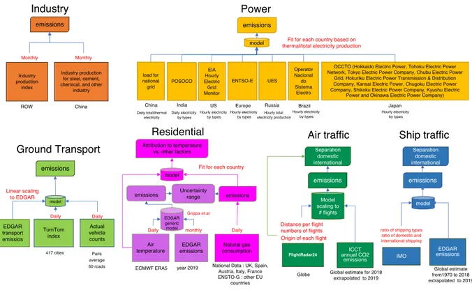
The framework of this study is illustrated in Fig. 1. We calculated national CO2 emissions and international
aviation and shipping emissions since January 1, 2019, drawing on hourly datasets of electric power production and the associated CO2 emissions in 31 countries (thus including the substantial variations in carbon intensity
associated with the variable mix of electricity production), daily vehicle traffic indices in 416 cities worldwide, monthly production data for cement, steel and other energy intensive industrial products in 62 countries/regions, daily maritime and aircraft transportation activity data, and previous-year fuel use data corrected for air temper-ature for residential and commercial buildings, covering over 70% of global power and industry emissions, 85% of ground transportation emissions, 100% of residential and international bunker emissions, respectively. We also inferred the emissions from ROW (see Methods) where data are not directly available thus covering 100% of global CO2 emissions. Together, these data cover almost all fossil fuels and industry sources of global CO2
emis-sions, except for emissions from land use change (up to 10% of global CO2 emissions), and the non-fossil fuel CO2
emissions of industrial products (up to 2% of global CO2 emissions)27 and of cement and clinker (e.g., plate glass,
ammonia, urea, calcium carbide, soda ash, ethylene, ferroalloys, alumina, lead and zinc).
While daily emissions can be directly calculated using near-real-time activity data and emission factors for the electricity power sector, such an approach is difficult to apply to all sectors. For the industrial sector, emis-sions can be estimated monthly in some countries. For the other sectors, we used proxy data instead of daily real activity data to dynamically downscale the annual or monthly CO2 emissions totals to a daily basis. For instance,
traffic indices in cities representative of each country were used instead of actual vehicle counts and categories, combined with annual national total sectoral emissions, to produce daily road transportation emissions. As such, for the use of fuels in the road transportation, air transportation and residential sectors in most countries, we downscaled monthly or annual total emissions data in 2019 to calculate the daily CO2 emissions in that year.
Subsequently, we scaled monthly totals of 2019 by daily proxies of activities to obtain daily CO2 emissions data
for the first four months of 2020 during the unprecedented disruption of the COVID-19 pandemic. The Carbon Monitor near-real-time CO2 emission dataset shows a 8.8% decline in CO2 emissions globally from January 1st
to June 30th in 2020 when compared with the same period in 2019 (Fig. 2), and detects a regrowth of CO 2
emis-sions by late April, which is mainly attributed to the recovery of economic activities in China and partial easing of lockdowns in other countries (for a more in-depth analysis of this topic, please see our recent related paper28).
Methods
annual total and sectoral emissions per country in the baseline year 2019.
According to the IPCC guidelines for emissions reporting4, the CO2 emissions Emis should be calculated by multiplying the
activ-ity data AD by the corresponding emissions factors EF
∑∑∑
= ⋅
Emis ADi j k, , EFi j k, , (1)
where i, j, k are indices for regions, sectors and fuel types, respectively. EF can be further separated into the net heating values v for each fuel type (the energy obtained per unit of fuel), the carbon content c per energy output (t C/TJ) and the oxidization rate o (the fraction (in %) of fuel oxidized during combustion):
∑∑∑
= ⋅ ⋅ ⋅
Emis ADi j k, , (vi j k, , ci j k, , oi j k, ,) (2) Due to the lag of more than two years in the publishing governmental energy statistics, we started from the most recent CO2 emissions estimates up to 2018 from current CO2 databases1,9–11. For 2019, we completed this
information by obtaining annual total emissions based on data in the literature and disaggregated the annual total
Fig. 1 Framework for data processing.
1/ 1 2/ 1 3/ 1 4/ 1 5/ 1 6/ 1 7/ 1 8/ 1 9/ 1 10/ 1 11/ 1 12/ 1 Emi ssions (Mt CO 2 pe rd ay ) 70 80 90 100 110 120
Global (-8.8% in Jan1st to Jun30th, 2020)
WU IT 2019 2020 Date WU Average (2019) Average (2020)
into daily emissions (see below). For 2020, we estimated daily CO2 emissions by using daily changes in activity
data in 2020 compared to 2019. The CO2 emissions and sectoral structure in 2018 for countries and regions were
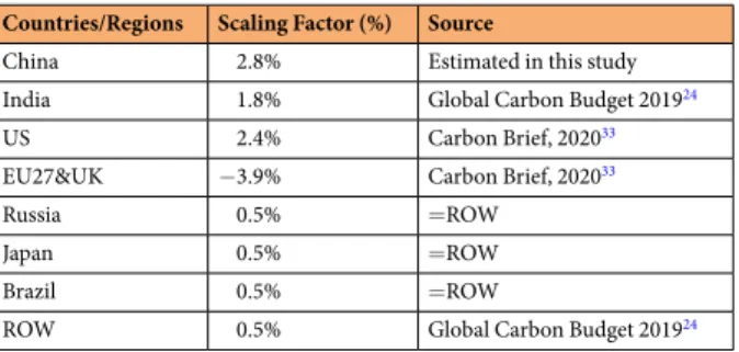
extracted from EDGAR V4.3.21 and V5.029 for each country, and national emissions were scaled to 2019 based
on our own estimate (for China) and data from the Global Carbon Budget 201924 (for other countries) (Table 1):
α
= ⋅
Emisr,2019 r Emisr,2018 (3)
For China, we first calculated CO2 emissions in 2018 based on the energy consumption by fuel type and for
cement production in 2018 from the China Energy Statistical Yearbook30 and the National Bureau Statistics31,
following Eq. 1. We projected the energy consumption in 2019 from the annual growth rates of coal, oil and gas reported by the Statistical Communiqué31 and applied China-specific emission factors17 to obtain the annual
growth rate of emissions in 2019. We projected China’s CO2 emissions based on our previous studies on the
country-specific emission factor data in China17 and past trends of China’s CO
2 emissions17,32. Our projection
(2.6%) is similar to the GCP revised projection33 (2.0%), and the slight difference falls into the uncertainty range
of the both estimations. For the US and EU27&UK, we used updated emissions growth rates in 2019 reported by CarbonBrief33. For countries with no estimates for emissions growth rates in 2019, such as Russia, Japan and
Brazil, we assumed that their growth rate was 0.5% based on the emission growth rate of the rest of the world24.
As the result, our daily average CO2 estimates in 2019 (98.2 Mt CO2 per day) are lower than the daily average CO2
estimates in 2019 from GCP (around 100 Mt CO2 per day). The discrepancies mainly came from the difference
between EDGAR and GCP databases, showing a 2.1% global difference between these two databases in 2018. In this study, the EDGAR detailed sectors were aggregated into several larger sectors (s): power sector, indus-trial sector, transport sector (ground transport, aviation and shipping), and residential sector, and the percentage estimates for the various sectors are derived from the EDGAR database. This is consistent with the new activity data we used below to compute daily variations. We used the sectoral distribution in 2018 from EDGAR to infer the sectoral emissions in 2019 for each country/region (Eq. 4), assuming that the sectoral distribution remained unchanged in these two years.
= ⋅
Emis Emis Emis
Emis (4)
r s r r s
r
, ,2019 ,2019 , ,2018 ,2018
Data acquisition and processing of carbon monitor daily CO
2emissions.
According to IPCCGuidelines4, the CO
2 emissions for each sector can be calculated by multiplying sectoral activity data by their
corresponding emission factors following Eq. 5:
= ⋅
Emiss AD EFs s (5)
The emissions were calculated following this equation separately for the power sector, the industrial sector, the transport sector, and the residential sector.
Power sector.
The CO2 emissions from the power sector can be calculated by adapting Eq. 5 withsector-specific activity data (i.e., electricity production in Russia and thermal electricity production in other countries) and the corresponding emission factors (Eq. 6):
= ⋅
Emispower ADpower EFpower (6)
Normally, the emission factors change slightly over time but can be assumed to remain constant over the two-year period considered in this study compared to the large changes in activity data. We present uncertainties due to the changes of fuel mix in thermal production (see Technical Validation). Thus, we assumed that emission factors remained unchanged in 2019 and 2020 and calculated the daily emissions as follows:
= ⋅
Emis Emis AD
AD (7)
daily yearly daily yearly
For China, we estimate the daily thermal production ADdaily from the daily disaggregation of monthly thermal emissions ADmonthly by using daily coal consumption by six power companies in China Cdaily as follow:
Countries/Regions Scaling Factor (%) Source
China 2.8% Estimated in this study India 1.8% Global Carbon Budget 201924
US 2.4% Carbon Brief, 202033
EU27&UK −3.9% Carbon Brief, 202033
Russia 0.5% =ROW Japan 0.5% =ROW Brazil 0.5% =ROW
ROW 0.5% Global Carbon Budget 201924
= ⋅
ADdaily ADmonthly (Cdaily/Cmonthly) (8)
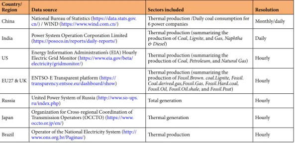
The data sources of daily activity data in the power sector are described in Table 2. The countries/regions listed in Table 2 account for more than 74% of the total CO2 emissions in the power sector. For emissions from other
countries (ROW), which are not listed in Table 2, we estimated the power sector emission changes in 2020 based on periods of the national lockdown. For daily emission changes for the ROW in 2019, we first assumed a linear relationship between daily global emissions and daily total emissions for the countries listed in Table 2. Then, we classified each country according to whether it adopted lockdown measures based on official reports. Based on daily emissions data for the power sector of the countries listed in Table 2, we calculated the average percent change α of power sector emissions across those countries during their lockdown periods, and used it to estimate the emission reduction of each country in the rest of the world during their specific national lockdowns (Eq. 9, where c denotes a country in ROW and d denotes day of 2020), and aggregated them into daily emissions for each ROW country.
α
= × − ∈
Emisc d c, ( ) Daily Mean Emisc,2019 (1 ) , ( )d c lockdown period inc (9)
Industrial sector: Industrial and cement production.
While daily production data are not directly available for industrial and cement production, the monthly CO2 emissions from the industrial and cementpro-duction sectors can be calculated by using monthly statistics of industrial propro-duction and daily data of electricity generation to disaggregate the monthly CO2 emissions into daily values. This calculation assumes a linear
rela-tionship between daily electricity generation for industry and daily industry production data to compute daily industry production.
The emissions from industrial production during fossil fuel combustion were calculated by multiplying the activity data (i.e., fossil fuel consumption data in the industrial sector) by the corresponding emissions factors by the type of fuel. Due to limited data availability, we assumed a linear relationship between daily industrial production and industrial fossil fuel use, and the emission factors remained unchanged. Therefore, the monthly emissions in 2019 for a country/region can be calculated by the following equation:
= ⋅
Emismontly,2019,r Emisyearly,2019,r (Pmonthly,2019,r yearly/P ,2019, ,i r) (10) The emissions from cement production during the chemical process of calcination of calcite were also calcu-lated with Eq. (10).
Specifically, for China, the emissions from the industrial sector were further divided into those for the steel, cement, chemical, and other industries (indicated by index i):
∑
= ⋅
Emismontly,2019,China Emisyearly,2019,i (Pmonthly,2019,i yearly/P ,2019,i) (11) For the monthly emissions in 2020 for a country/region, we used the following equation:
= ⋅
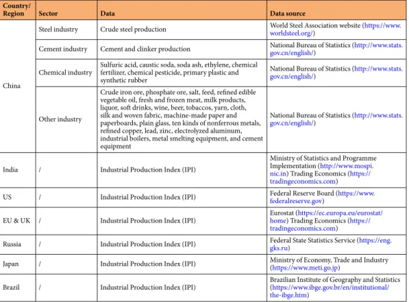
Emismontly,2020,r Emismonthly,2019,r (Pmonthly,2020,r monthly/P ,2019,r) (12) where P is the industrial production for different industrial sectors (in China) or the total industrial production index (in other countries), as listed in Table 3. In China’s case, the January and February estimates were combined, as individual monthly data were not reported by the sources listed in Table 3 for these two months. The monthly industrial emissions were disaggregated to daily emissions using daily electricity data, as explained above.
Country/
Region Data source Sectors included Resolution
China National Bureau of Statistics (cn/) / WIND (https://www.wind.com.cn/https://data.stats.gov.) Thermal production /Daily coal consumption for 6 power companies Monthly/daily
India Power System Operation Corporation Limited (https://posoco.in/reports/daily-reports/) Thermal production (summarizing the production of Coal, Lignite, and Gas, Naphtha
& Diesel) Daily
US Energy Information Administration’s (EIA) Hourly Electric Grid Monitor (https://www.eia.gov/beta/ electricity/gridmonitor/)
Thermal production (summarizing the
production of Coal, Petroleum, and Natural Gas) Hourly
EU27 & UK ENTSO-E Transparent platform (transparency.entsoe.eu/dashboard/showhttps://)
Thermal production (summarizing the production of Fossil.Brown. coal.Lignite, Fossil.
Coal.derived.gas,Fossil.Gas, Fossil.Hard.coal, Fossil.Oil, Fossil.Oil.shale, and Fossil.Peat)
Hourly
Russia United Power System of Russia (ru/index.php) http://www.so-ups. Total generation Hourly
Japan Organization for Cross-regional Coordination of Transmission Operators (OCCTO) (https://www.
occto.or.jp/en/) Thermal generation Hourly
Brazil Operator of the National Electricity System (www.ons.org.br/Paginas/) http:// Thermal production Hourly
Lacking the latest Industrial Production Index for June 2020 for the EU27 & UK and India, we adopted monthly growth rates of industrial output from Trading Economics (https://tradingeconomics.com) based on preliminary survey data. CO2 emissions from countries listed in Table 3 accounts for more than 71% of the global
industrial emissions. For other countries not listed in Table 3, we used the same method described for the power sector to calculate the daily industry emissions from the ROW.
To allocate monthly emissions into daily emissions, we assume the linear relationship between daily industry activity and daily electricity production, and use the weight of daily electricity production to monthly electricity production:
= ⋅
Emisdaily Emismonthly (Elecdaily/Elecmonthly) (13)
transport sector.
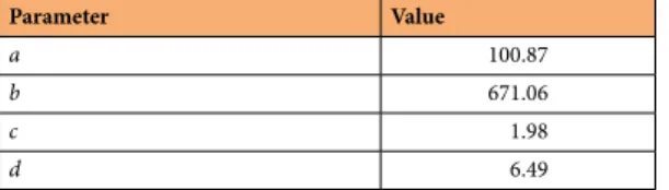
Ground transportation. We collected hourly congestion level data from the TomTomwebsite (https://www.tomtom.com/en_gb/traffic-index/). The congestion level (hereafter called X) represents the extra time spent on a trip, as a percentage, compared to under uncongested conditions. TomTom congestion level data were obtained for 416 cities across 57 countries (Only-online Table 1) at a temporal resolution of one hour. Of note, a zero-congestion level means that the traffic is fluid or ‘normal’ but does not mean there are no vehicles and zero emissions. It is thus important to identify the lower threshold of emissions when the congestion level is zero. To do so, we compared the time series of daily mean TomTom congestion level X with the daily mean car flux (in vehicles per day) from publicly available real-time Q data from an average of 60 roads in the megacity area of Paris. The daily mean car counts were reported by the city’s service (https://opendata.paris.fr/pages/home/). We used a sigmoid function to fit the relationship between X and Q:
= + + Q a bX d X (14) c c c
where a, b, c and d are the regression parameters (Table 4). We verified that the empirical fit from Eq. 14 can reproduce the observed large drop in Q due to the lockdown in Paris and the recovery afterwards. We assume that relative changes in daily emissions were proportional to the relative change in the function Q(X) from Eq. 14. Then, we applied the function Q(X) established for Paris to other cities included in the TomTom dataset, assuming that the relative magnitude of car counts (and thus emissions) follows a similar relationship with TomTom. The emission changes were first calculated for individual cities and then weighted by city emissions for aggregation to national changes. For a specific country i with n cities reported by TomTom, the national daily vehicle flux for day j was given by:
= ∑ ∑ = = Q Q E E (15) country dayj i n i dayj i i n i , 1 , 1
where Ei is the annual road transportation emissions of city n taken at the grid point of each TomTom city from the annual gridded EDGARv4.3.2 emissions map for the “road transportation” sector (1A3b) (https://edgar.jrc. ec.europa.eu/) for the year 2010, assuming that the spatial distribution of ground transport did not change signif-icantly within a country between 2010 and the period of this study. Then, the daily road transportation emissions in 2019 and 2020 (Ecountry dayj, ) for a country were scaled such that the total road transportation emissions in the
first half year of 2019 equaled 182/365 times the annual emissions of this sector in 2019 (Ecountry,2019) estimated in
this study: = × ∑= E Q E Q 182/365 (16)
country dayj country dayj country j country dayj
, , ,2019
1 182
, (2019)
The TomTom GPS products include devices for car (https://www.tomtom.com/en_us/drive/car/), motorcycle (https://www.tomtom.com/en_us/drive/motorcycle/) and large vehicles (https://www.tomtom.com/en_us/drive/ truck/). Although we did not find more information about the details how the congestion index is calculated, we believe that the calculation of congestion level includes the data from private and commercial cars, light and heavy vehicles. In this study, we did not compute the emissions separately for light and heavy vehicles sepa-rately, because 1) the EDGAR emission product for “road transport” (sector 1A3b), which we used as a reference emission product, did not separate these two different types of vehicles; and 2) the TomTom congestion level is not reported for light and heavy vehicles separately. So we implicitly assume that they similarly scale with the TomTom congestion level.
For countries not included in the TomTom dataset, we assumed that the emissions changes follow the mean changes of other countries. For example, Cyprus, as an EU member country, had no city reported in the TomTom dataset, so its relative emissions change was assumed to follow the same pattern for total emissions from other EU countries included in the TomTom dataset (which covers 98% of total EU emissions). Similarly, the relative changes in emissions for countries in the ROW but not reported by TomTom were assumed to follow the same pattern as the total emissions from all TomTom reported countries (which cover 85% of global total emissions).
Aviation. CO2 emissions from commercial aviation are usually reconstructed from bottom-up emission
inven-tories based on knowledge of the parameters of individual flights34,35. We also calculated the CO
2 emissions from
commercial aviation following this approach. Individual commercial flights are tracked by Flightradar24 (https:// www.flightradar24.com) based on ADS-B signals emitted by aircraft and received by their network of ADS-B
receptors. As we do not yet have the capability to convert the FlightRadar24 database into CO2 emissions on
a flight-by-flight basis, we compute CO2 emissions by assuming a constant EFaviation (CO2 emission factor per
km flown) across the whole fleet of aircraft (regional, narrowbody passenger, widebody passenger and freight operations). This assumption is reasonable if the flight mix between these categories has not changed signifi-cantly between 2019 and 2020.The International Council on Clean Transportation (ICCT) published that CO2
emissions from commercial freight and passenger aviation resulted in 918 Mt CO2 in 201836 based on the OAG
flight database and emission factors from the PIANO database. IATA estimated a 3.4% increase between 2018 and 2019 in terms of available seat kilometers37. In the absence of further information, we consider this increase to be
representative of freight aviation as well and use a slightly smaller growth rate of 3% for CO2 emissions between
2018 and 2019 to account for a small increase in fuel efficiency. The kilometers flown are computed assuming great circle distance between the take-off, cruising, descent and landing points for each flight and are cumulated over all flights. The FlightRadar24 database has incomplete data for some flights and may completely miss a small fraction of actual flights, so we scale the ICCT estimate of CO2 emissions (inflated by 3% for 2019) with the total
estimated number of kilometers flown for 2019 (67.91 million km) and apply this scaling factor to 2020 data. Again, this assumes that the fraction of missed flights is the same in 2019 and 2020. As the departure and landing airports are known for each flight, we can classify the km flown (and hence the CO2 emissions) per country and
for each country between domestic or international traffic. The daily CO2 emissions were computed as the
prod-uct of distance flown by a CO2 emission factor per km flown, according to:
= ×
Daily Emisaviation Daily Kilometers Flownaviation2020 EFaviation2019 (17)
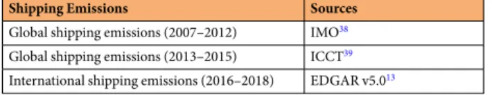
Ships. We collected international CO2 shipping emissions for 2016–2018 based on EDGAR’s international
emis-sions. We also collected global shipping emissions during the period of 2007–2015 from IMO38 and ICCT39.
According to the Third IMO GHG Study38, CO
2 emissions from international shipping accounted for 88% of
global shipping emissions, and domestic and fishing emissions accounted for 8% and 4%, respectively. We cal-culated international CO2 shipping emissions from 2007–2015 from global shipping emissions and the ratio of
international to global shipping emissions. We extrapolated emissions from linear fits from 2007–2018 to estimate the emissions in 2019. The data sources of shipping emissions are listed in Table 5. We obtained emissions for the first half year of 2019 byassuming the equal distribution of monthly shipping CO2 emissions. The equations are
as follows:
α
= × ×
Monthly Emisinternational shipping,2019 Yearly Emisinternational shipping,2019 Rmonth (18) α is the increasing rate of international shipping emissions in 2019 based on the linear extrapolation of data from the period 2007–2018, estimated to be 3.01%. Rmonth represents the ratio of the months to be calculated in
Country/
Region Sector Data Data source
China
Steel industry Crude steel production World Steel Association website (worldsteel.org/) https://www.
Cement industry Cement and clinker production National Bureau of Statistics (gov.cn/english/) http://www.stats.
Chemical industry Sulfuric acid, caustic soda, soda ash, ethylene, chemical fertilizer, chemical pesticide, primary plastic and synthetic rubber
National Bureau of Statistics (http://www.stats. gov.cn/english/)
Other industry
Crude iron ore, phosphate ore, salt, feed, refined edible vegetable oil, fresh and frozen meat, milk products, liquor, soft drinks, wine, beer, tobaccos, yarn, cloth, silk and woven fabric, machine-made paper and paperboards, plain glass, ten kinds of nonferrous metals, refined copper, lead, zinc, electrolyzed aluminum, industrial boilers, metal smelting equipment, and cement equipment
National Bureau of Statistics (http://www.stats. gov.cn/english/)
India / Industrial Production Index (IPI)
Ministry of Statistics and Programme Implementation (http://www.mospi. nic.in) Trading Economics (https:// tradingeconomics.com)
US / Industrial Production Index (IPI) Federal Reserve Board (federalreserve.gov) https://www.
EU & UK / Industrial Production Index (IPI) Eurostat (home) Trading Economics (https://ec.europa.eu/eurostat/https:// tradingeconomics.com)
Russia / Industrial Production Index (IPI) Federal State Statistics Service (gks.ru) https://eng. Japan / Industrial Production Index (IPI) Ministry of Economy, Trade and Industry (https://www.meti.go.jp)
Brazil / Industrial Production Index (IPI) Brazilian Institute of Geography and Statistics (https://www.ibge.gov.br/en/institutional/ the-ibge.htm)
the whole year. Given this, we estimated the shipping emissions for the first half year of 2019 using Rmonth equal to
181/365.
We assumed that the change in shipping emissions was linearly related to the change in ship traffic volume. The change in international shipping emissions for the first half year of 2020 was calculated according to the following equation:
= ×
Emisperiod,2020 Emisperiod,2019 Cindex (19)
where cindex represents the ratio of the change in shipping emissions, estimated to the end of April as −25% com-pared to the same period last year according to the news report40.
residential sector: residential and commercial buildings.
Fuel consumption daily data from this sector are not available. Several studies41,42 showed that the main source of daily and monthly variability in thissector is climate, namely, heating emissions increase when temperature falls below a threshold that depends on the region, building type and people’s habits. We calculated emissions by assuming annual totals unchanged from 2019 and using daily climate information in three steps: 1) estimate population-weighted heating degree days for each country and for each day based on the ERA543 reanalysis of 2-meter air temperature, 2) split residential
emissions into two parts: cooking emissions and heating emissions based on the EDGAR database29 and using the
EDGAR estimates of 2018 residential emissions as the baseline. Emissions from cooking were assumed to remain independent of temperature, and those from heating were assumed to be a function of the heating demand. Based on the change in population-weighted heating degree days in each country in 2019 and 2020, we downscaled annual EDGAR 2018 residential emissions to daily values for 2019 and 2020 as described by Eqs. 20–22:
= × ∑ ∑ Emis Emis HDD HDD (20) c m c m c d c d , , ,2018 m , m,2018 , = × × ∑ + × − ×
Emis Emis Ratio HDD
HDD Emis (1 Ratio ) N 1 (21) c d c m heating c m c d c d c m heating c m m , , , , , m , , , ,
∑
∑
= ×(
−)
HDD Pop T Pop ( 18 ) ( ) (22) c d grid grid c d grid , , ,where c is country, d is day, m is month, Emisc m, is the residential emissions of country c in month m of year 2019
or 2020, Emisc m, ,2018is the emissions of country c in month m of year 2018, HDDc d, is the population-weighted
heating degree day in country c in day d, Emisc d, is the residential emissions of country c in day d of year 2019 or
2020, Ratioheating c m, , is the percentage of residential emissions from heating demand in country c in month m, Nm is the number of days in month m, Popgrid is gridded population data derived from Gridded Population of the World, Version 444, T is the daily average air temperature at 2 meters derived from ERA543, and 18 is a HDD
ref-erence temperature13 of 18 °C.
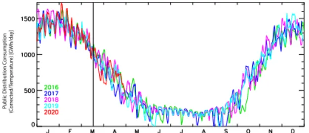
The main assumption in this approach is that residential emissions did not change based on factors other than heating degree day variations in 2020, although people’s time at home dramatically increased during the lock-down period. To test the validity of this assumption, we compiled natural gas daily consumption data by residen-tial and commercial buildings for France (https://www.smart.grtgaz.com/fr/consommation) (unfortunately, such data could not be collected in many countries) during 2019 and 2020 (Fig. 3). Natural gas consumption in kWh per day was transformed to CO2 emissions using an emission factor of 10.55 kWh per m3 and a molar volume of
22.4 10−3 m3 per mole.
First, we verified that the temporal variation in those ‘true’ residential CO2 emissions was similar to that given
by Eqs. 20–22. Second, after fitting a piecewise model to those natural gas residential emission data using ERA5 air temperature data, we removed the effect of temperature to obtain emissions corrected for temperature effects. Even if the lockdown was very strict in France, we found no significant emissions anomaly, meaning that although nearly the entire population was confined at home, it did not increase or decrease emissions. This complementary analysis tentatively suggests that residential emissions can be well approximated in other countries by Eqs. 20–22
based only on temperature during the lockdown period.
Parameter Value
a 100.87
b 671.06
c 1.98
d 6.49
Table 4. Regression parameters of the sigmoid function of Eq. 14 that describes the relationship between car counts (Q) and TomTom congestion level (X).
Data Records
Currently, there are 36,177 data records provided in this dataset, which can be downloaded at our website (https:// carbonmonitor.org) and Figshare45:
• A total of 270 records are daily mean CO2 emissions (from fossil fuel combustion and cement production
processes) 1751–2020.
• A total of 4,923 records are the daily emissions for 9 countries/regions (i.e. China, India, US, EU27 & UK, Russia, Japan, Brazil, ROW and World) and 547 days (from January 1, 2019 to June 30th, 2020).
• A total of 3,829 records are the daily emissions for 6 sectors and the global total (i.e. power, industry, residen-tial, ground transportation, aviation (including domestic aviation and international aviation), international shipping and Globe) and 547 days (from January 1, 2019 to June 30th, 2020).
• A total of 27,155 records are daily emissions of 9 countries/regions (i.e. China, India, US, EU27 & UK, Russia, Japan, Brazil, ROW and World) in the power sector and industrial sector and the global total in the interna-tional shipping sector for 547 days (from January 1, 2019, to June 30th, 2020), and ground transport sector,
residential sector and aviation sector (China, India, US, EU27 & UK, Russia, Japan, Brazil, ROW, domestic aviation total, international aviation, and total aviation) for 578 days (from January 1, 2019, to July 31st, 2020).
technical Validation
Uncertainty estimates.
We calculate daily emissions directly from daily activity data in most sectors, thus the daily uncertainties are explained by the specific uncertainty of daily sectoral activity data itself and uncertain-ties in the (empirical) models used to convert activity to emissions. Here we should distinguish between error and uncertainty. Errors being defined the difference to the truth cannot be estimated because we do not know the true values. Uncertainty could be estimated if we had different activity datasets, by looking at the spread of these different datasets, but this is also not possible as most of our activity data are unique. The main issue is that we do not know if the uncertainty of activity data would be a systematic uncertainty (e.g. all days are biased low using our activity dataset compared to another activity dataset) or a random error (in which case, there could be posi-tive bias one day compensated by negaposi-tive bias another day and the uncertainty would be small e.g. on monthly values derived from daily values). We do acknowledge that we cannot estimate daily uncertainties. In the future, this could be done by trying to collect different activity data. This uncertainty analysis was also presented in our related paper recently published at Nature Communications28.Thus, we followed the 2006 IPCC Guidelines for National Greenhouse Gas Inventories to conduct an uncer-tainty analysis of the data. First, the uncertainties were calculated for each sector (See Table 6 for uncertainty ranges of each sector):
• Power sector: the uncertainty is mainly from inter-annual variability of coal emission factors and changes in mix of generation fuel in thermal production. The uncertainty of power emission from fossil fuel is within (±14%) with the consideration of both inter-annual variability of fossil fuel based on the UN statistics and the variability of the mix of generation fuel (the ratio of electricity produced by coal to thermal production). • Industrial sector: The uncertainty of CO2 from industry and cement production comes from monthly
pro-duction data. CO2 from industry and cement production in China accounts for more than 60% of world total
industrial CO2, and the uncertainty of emissions in China is 20%. Uncertainty from monthly statistics was
derived from 10,000 Monte Carlo simulations to estimate a 68% confidence interval (1 sigma) for China. We calculated the 68% prediction interval of the linear regression models between emissions estimated from monthly statistics and official emissions obtained from annual statistics at the end of each year to deduce the one-sigma uncertainty involved when using monthly data to represent the change for the whole year. The squared correlation coefficients are within the range of 0.88 (e.g., coal production) and 0.98 (e.g., energy import and export data), which indicates that only using the monthly data can explain 88% to 98% of the whole year’s variation32; the remaining variation is not covered but reflects the uncertainty caused by the
frequent revisions of China’s statistical data after they are first published.
• Ground Transportation: The emissions from the ground transportation sector are estimated by assuming that the relative magnitude in car counts (and thus emissions) follow a similar relationship with TomTom conges-tion index in Paris. This model calibrated in Paris was cross checked to match traffic fluxes of two other cities. Future work will focus on additional cross-validation and calibration with more traffic data from other cities. • Aviation: The uncertainty in the aviation sector comes from the difference in daily emission data estimated
based on the two methods. We calculate the average difference between the daily emission results estimated based on the flight route distance and the number of flights and then divide the average difference by the aver-age daily emissions estimated by the two methods to obtain the uncertainty in CO2 from the aviation sector.
• Shipping: We used the uncertainty analysis from IMO as our uncertainty estimate for shipping emissions. According to the Third IMO Greenhouse Gas study 201438, the uncertainty in shipping emissions was 13%
based on bottom-up estimates.
Shipping Emissions Sources
Global shipping emissions (2007–2012) IMO38
Global shipping emissions (2013–2015) ICCT39
International shipping emissions (2016–2018) EDGAR v5.013
• Residential: The 2-sigma uncertainty in daily emissions is estimated as 40%, which is calculated based on a comparison with daily residential emissions derived from real fuel consumption in several European coun-tries, including France, Great Britain, Italy, Belgium, and Spain.
The uncertainty in the emission projection for 2019 is estimated as 2.2% by combining the reported uncer-tainty of the projected growth rates and the EDGAR estimates in 2018.
Then, we combine all the uncertainties by following the error propagation equation from the IPCC. Equation 23 is used to derive the uncertainty of the sum and could be used to combine the uncertainties of all sectors:
∑
∑
µ µ = ⋅ U (U ) (23) total s s swhere Us and µs are the percentage and quantity (daily mean emissions) of the uncertainty of sector s,
respectively.
Equation 24 is used to derive the uncertainty of the multiplication, which in turn is used to combine the uncertainties of all sectors and of the projected emissions in 2019:
∑
=
Uoverall Ui2 (24)
Code availability
The generated datasets are available from https://doi.org/10.6084/m9.figshare.12685937.v4 and https://github. com/zhudeng94/dailyCO2. Codes for industrial emission calculation and summary table generation are available on the GitHub repository presented as worksheets. Also the raw data of power generation in U.S., EU27 & UK, India, Russia, Japan and Brazil are available on the GitHub repository. Other raw data and codes for emission estimation in other sectors are only available upon reasonable requests.
Received: 10 June 2020; Accepted: 17 September 2020; Published: xx xx xxxx
References
1. Janssens-Maenhout, G. et al. EDGAR v4.3.2 Global Atlas of the three major Greenhouse Gas Emissions for the period 1970–2012.
Earth Syst. Sci. Data 11, 959–1002 (2019).
2. Marland, G. & Rotty, R. M. Carbon dioxide emissions from fossil fuels: a procedure for estimation and results for 1950–1982. Tellus
Ser. B-Chem. Phys. Meteorol. 36, 232–261 (1984).
Fig. 3 Residential and commercial building daily natural gas consumption (linearly related to CO2 emissions
from this sector) in France for the last 5 years. Temperature effects have been removed from emissions using a linear piecewise model fitted to daily data. When the effect of variable winter temperature was removed, no significant change is seen in 2020 during the very strict lockdown period except for a small dip by end of March.
Items Uncertainty Range
Power ±14.0% Ground transport ±9.3% Industry ±36.0% Residential ±40.0% Aviation ±10.2% International shipping ±13.0% Projection of emissions growth rate in 2019 ±0.8% EDGAR emissions in 2018 ±5.0%
Overall ±7.2%
3. Intergovernmental Panel on Climate Change (IPCC). Revised 1996 IPCC Guidelines for National Greenhouse Gas Inventories. (Intergovernmental Panel on Climate Change, 1997).
4. Eggleston, S., Buendia, L., Miwa, K., Ngara, T. & Tanabe, K. 2006 IPCC guidelines for national greenhouse gas inventories. Vol. 5 (Institute for Global Environmental Strategies Hayama, Japan, 2006).
5. Gregg, J. S., Andres, R. J. & Marland, G. China: Emissions pattern of the world leader in CO2 emissions from fossil fuel consumption
and cement production. Geophys. Res. Lett. 35, GL032887 (2008).
6. Andres, R. J., Boden, T. A. & Higdon, D. A new evaluation of the uncertainty associated with CDIAC estimates of fossil fuel carbon dioxide emission. Tellus Ser. B-Chem. Phys. Meteorol. 66 (2014).
7. Fridley, D., Zheng, N. & Qin, Y. Inventory of China’s Energy-Related CO2 Emissions in 2008. (Lawrence Berkeley National Laboratory,
2011).
8. Andres, R. J., Gregg, J. S., Losey, L., Marland, G. & Boden, T. A. Monthly, global emissions of carbon dioxide from fossil fuel consumption. Tellus Ser. B-Chem. Phys. Meteorol. 63, 309–327 (2011).
9. Le Quéré, C. et al. Global carbon budget 2018. Earth Syst. Sci. Data 10, 2141–2194 (2018).
10. BP. Statistical Review of World Energy, https://www.bp.com/en/global/corporate/energy-economics/statistical-review-of-world-energy.html (2020).
11. International Energy Agency (IEA). CO2 Emissions from Fuel Combustion 2019,
https://www.iea.org/reports/co2-emissions-from-fuel-combustion-2019 (2019).
12. Hong, C. et al. Variations of China’s emission estimates: response to uncertainties in energy statistics. Atmos. Chem. Phys. 17, 1227–1239 (2017).
13. Crippa, M. et al. High resolution temporal profiles in the Emissions Database for Global Atmospheric Research. Sci. Data 7, 121 (2020).
14. Zhao, Y., Zhou, Y., Qiu, L. & Zhang, J. Quantifying the uncertainties of China’s emission inventory for industrial sources: From national to provincial and city scales. Atmos. Environ. 165, 207–221 (2017).
15. Andres, R. J. et al. A synthesis of carbon dioxide emissions from fossil-fuel combustion. Biogeosciences 9, 1845–1871 (2012). 16. Olivier, J. G., Janssens-Maenhout, G. & Peters, J. A. Trends in global CO2 emissions: 2013 report. Report No. 9279253816, (PBL
Netherlands Environmental Assessment Agency, 2013).
17. Liu, Z. et al. Reduced carbon emission estimates from fossil fuel combustion and cement production in China. Nature 524, 335–338 (2015).
18. Choudhury, A., Roy, J., Biswas, S., Chakraborty, C. & Sen, K. Determination of carbon dioxide emission factors from coal combustion. In Climate Change and India: Uncertainty Reduction in Greenhouse Gas Inventory Estimates (Universities Press, 2004). 19. Roy, J., Sarkar, P., Biswas, S. & Choudhury, A. Predictive equations for CO2 emission factors for coal combustion, their applicability
in a thermal power plant and subsequent assessment of uncertainty in CO2 estimation. Fuel 88, 792–798 (2009).
20. Sarkar, P. et al. Revision of country specific NCVs and CEFs for all coal categories in Indian context and its impact on estimation of CO2 emission from coal combustion activities. Fuel 236, 461–467 (2019).
21. OlivierJ. G. J. & Peters, J. A. H. W. Trends in global CO2 and total greenhouse gas emissions; 2019 Report. (PBL Netherlands
Environmental Assessment Agency, The Hague, 2019).
22. Andres, R. J., Boden, T. A. & Higdon, D. M. Gridded uncertainty in fossil fuel carbon dioxide emission maps, a CDIAC example.
Atmos. Chem. Phys. 16 (2016).
23. Asefi‐Najafabady, S. et al. A multiyear, global gridded fossil fuel CO2 emission data product: Evaluation and analysis of results. J.
Geophys. Res.: Atmos. 119, 10,213–210,231 (2014).
24. Friedlingstein, P. et al. Global carbon budget 2019. Earth Syst. Sci. Data 11, 1783–1838 (2019).
25. Oda, T., Maksyutov, S. & Andres, R. J. The Open-source Data Inventory for Anthropogenic CO2, version 2016 (ODIAC2016): a
global monthly fossil fuel CO2 gridded emissions data product for tracer transport simulations and surface flux inversions. Earth
Syst. Sci. Data 10, 87–107 (2018).
26. Gregg, J. S. & Andres, R. J. A method for estimating the temporal and spatial patterns of carbon dioxide emissions from national fossil-fuel consumption. Tellus Ser. B-Chem. Phys. Meteorol. 60, 1–10 (2008).
27. Cui, D., Deng, Z. & Liu, Z. China’s non-fossil fuel CO2 emissions from industrial processes. Appl. Energy 254, 113537 (2019).
28. Liu, Z., Ciais, P., Deng, Z. et al. Near-real-time monitoring of global CO2 emissions reveals the effects of the COVID-19
pandemic. Nat Commun 11, 5172 (2020).
29. Crippa, M. et al. Fossil CO2 and GHG emissions of all world countries - 2019 Report. (Publications Office of the European Union,
2019).
30. National Bureau of Statistics. China Energy Statistical Yearbook. (China Statistical Press, 2019).
31. National Bureau of Statistics. Statistical Communiqué of the People’s Republic of China on the National Economic and Social
Development, http://www.stats.gov.cn/tjsj/tjgb/ndtjgb/ (2020).
32. Liu, Z., Zheng, B. & Zhang, Q. New dynamics of energy use and CO2 emissions in China. Preprint at https://arxiv.org/abs/1811.09475
(2018).
33. Korsbakken, J. I., Andrew, R. & Peters, G. Guest post: Why China’s CO2 emissions grew less than feared in 2019, https://www.
carbonbrief.org/guest-post-why-chinas-co2-emissions-grew-less-than-feared-in-2019 (2020).
34. Ji-Cheng, H. & Yu-Qing, X. Estimation of the Aircraft CO2 Emissions of China’s Civil Aviation during 1960–2009. Adv. Clim. Chang.
Res. 3, 99–105 (2012).
35. Turgut, E. T., Usanmaz, O. & Cavcar, M. The effect of flight distance on fuel mileage and CO2 per passenger kilometer. Inter. J.
Sustain. Transp. 13, 224–234 (2019).
36. Graver, B., Zhang, K. & Rutherford, D. CO2 emissions from commercial aviation, 2018. (International Council on Clean
Transportation, 2019).
37. International Air Transport Association (IATA). Slower but Steady Growth in 2019, https://www.iata.org/en/pressroom/pr/2020-02-06-01/ (2020).
38. Smith, T. W. P. et al. Third IMO Greenhouse Gas Study 2014. (International Maritime Organization, London, UK, 2015).
39. Olmer, N., Comer, B., Roy, B., Mao, X. & Rutherford, D. Greenhouse Gas Emissions From Global Shipping, 2013–2015. (International Council on Clean Transportation, 2017).
40. Kinsey, A. Coronavirus Intensifies Global Shipping Risks, https://www.maritime-executive.com/editorials/coronavirus-intensifies-global-shipping-risks (2020).
41. Spoladore, A., Borelli, D., Devia, F., Mora, F. & Schenone, C. Model for forecasting residential heat demand based on natural gas consumption and energy performance indicators. Appl. Energy 182, 488–499 (2016).
42. VDI. Berechnung der Kosten von Wärmeversorgungsanlagen (Economy calculation of heat consuming installations) (VID-Gesellschaft Bauen und Gebäudetechnik. 1988).
43. Copernicus Climate Change Service (C3S). ERA5: Fifth generation of ECMWF atmospheric reanalyses of the global climate.
Copernicus Climate Change Service Climate Data Store https://cds.climate.copernicus.eu (2019).
44. Doxsey-Whitfield, E. et al. Taking advantage of the improved availability of census data: a first look at the gridded population of the world, version 4. Appl. Geogr. 1, 226–234 (2015).
45. Deng, Z. et al. Daily updated dataset of national and global CO2 emissions from fossil fuel and cement production. figshare https://
acknowledgements
Authors acknowledged reviews comment to improving the manuscript. Zhu Liu acknowledges funding from Qiushi Foundation, the Resnick Sustainability Institute at California Institute of Technology, Natural Science Foundation of Beijing (JQ19032) and the National Natural Science Foundation of China (grant 71874097 and 41921005).
author contributions
Zhu Liu and Philippe Ciais designed the research, and Zhu Deng coordinated the data processing. Zhu Liu, Philippe Ciais and Zhu Deng contributed equally to this research, and all authors contributed to data collection, analysis and paper writing.
Competing interests
The authors declare no competing interests.
additional information
Correspondence and requests for materials should be addressed to Z.L., P.C. or S.J.D. Reprints and permissions information is available at www.nature.com/reprints.
Publisher’s note Springer Nature remains neutral with regard to jurisdictional claims in published maps and institutional affiliations.
Open Access This article is licensed under a Creative Commons Attribution 4.0 International License, which permits use, sharing, adaptation, distribution and reproduction in any medium or format, as long as you give appropriate credit to the original author(s) and the source, provide a link to the Cre-ative Commons license, and indicate if changes were made. The images or other third party material in this article are included in the article’s Creative Commons license, unless indicated otherwise in a credit line to the material. If material is not included in the article’s Creative Commons license and your intended use is not per-mitted by statutory regulation or exceeds the perper-mitted use, you will need to obtain permission directly from the copyright holder. To view a copy of this license, visit http://creativecommons.org/licenses/by/4.0/.
The Creative Commons Public Domain Dedication waiver http://creativecommons.org/publicdomain/zero/1.0/
applies to the metadata files associated with this article. © The Author(s) 2020