HAL Id: halshs-00368422
https://halshs.archives-ouvertes.fr/halshs-00368422
Submitted on 16 Mar 2009
HAL is a multi-disciplinary open access archive for the deposit and dissemination of sci-entific research documents, whether they are pub-lished or not. The documents may come from teaching and research institutions in France or abroad, or from public or private research centers.
L’archive ouverte pluridisciplinaire HAL, est destinée au dépôt et à la diffusion de documents scientifiques de niveau recherche, publiés ou non, émanant des établissements d’enseignement et de recherche français ou étrangers, des laboratoires publics ou privés.
How Do Spouses Share their Full Income in Russia?:
Identification of the Sharing Rule Using Self-reported
Income
Ekaterina Kalugina, Natalia Radtchenko, Catherine Sofer
To cite this version:
Ekaterina Kalugina, Natalia Radtchenko, Catherine Sofer. How Do Spouses Share their Full Income in Russia?: Identification of the Sharing Rule Using Self-reported Income. Review of Income and Wealth, Wiley, 2009, 55 (2), pp.360-391. �10.1111/j.1475-4991.2009.00323.x�. �halshs-00368422�
How Do Spouses Share their Full Income in Russia?:
Identification of the Sharing Rule Using Self-reported Income
Ekaterina Kalugina1 (University of Paris 1-Panthéon-Sorbonne, CNRS, and HCE, Moscow)Natalia Radtchenko2 (University of Paris 1-Panthéon-Sorbonne, CNRS, & CREST-LMI) Catherine Sofer3 (University of Paris 1-Panthéon-Sorbonne, CNRS, and Paris School of
Economics) January 2007
The paper applies the collective model to the analysis of intra-household inequality using self-reported income scales and provides a test for its assumptions. We assume a correspondence between the income level that household members report and their true income sharing. Using Russian data, we first show that this assumption is supported by the data, and then use couples who report the same level of income to identify the full sharing rule for the whole sample. From simulations for an average couple living in the Urals, we find that a full income share of 45% is allocated to the wife.
JEL Classification: D1, J22, C3.
Keywords: Collective model, Within-household income comparisons, Subjective data,
Russia, Sharing rule.
1 CES, Maison des Sciences Economiques, 106-112, bd de l'Hôpital, 75647 PARIS cedex 13, France. Tel:
0033-1-44-07-82-52. E-mail: Ekaterina.Kalugina@malix.univ-paris1.fr
2 CES, Maison des Sciences Economiques, 106-112, bd de l'Hôpital, 75647 PARIS cedex 13, France. Tel:
0033-1-44-07-82-52. E-mail: Natalia.Radtchenko@malix.univ-paris1.fr
3 CES, Maison des Sciences Economiques, 106-112, bd de l'Hôpital, 75647 PARIS cedex 13, France. Tel:
INTRODUCTION
One central issue in applications of the economics of the household to policy analysis is that of within-household welfare comparisons and, in particular, of intra-family inequality. The current article examines this issue in the framework of a collective model of household behavior.
We provide an application of the collective model to the analysis of intra-household inequality, using self-reported income scales. The collective model based on the sharing rule (Chiappori, 1988, 1992 and 1997, Apps and Rees, 1997)) is used to determine empirically the intra-household allocation of resources formally represented by the sharing rule. Most of empirical applications are limited to identify the sharing rule up to a constant. This constraint comes from the non observation of the private consumption. We propose to use self-reported income scale as an additional source of identification allowing the full sharing rule retrieval.
. We interpret intra-household equality as the equal4 distribution of self-reported full income between the (main two adult) members of the household. Following recent models by Apps and Rees (1997), Chiappori (1997), Rapoport, Sofer and Solaz (2003 and 2006), and Bourguignon and Chiuri (2005), not only labor and non-labor income but also the output of household production are included in the household resources to be shared. We consider that such an approach better reflects the true consumption of leisure by both members of the household than that found in more standard collective models.
Using the framework of the collective model including household production under the assumption of marketable domestic goods (Rapoport, Sofer and Solaz, 2003 and 2006), we make a number of assumptions linking self-reported income and the theoretical results of the model. More precisely, we assume that the answers to a question in the data about
reported income reflect the true division of income within the family. This assumption is tested and we show that it is not refuted by the data. Then from the results obtained for the sub-sample of couples reporting the same level of income, we calculate the constant of the sharing rule for the whole sample: we thus propose a new method for deriving not only the derivatives, but also the sharing rule itself (see Browning, Chiappori and Lewbel, 2004).
In recent years a large number of empirical papers have analyzed self-reported income and poverty (Ferrer-i-Carbonell and Frijters, 2004). In this paper we assume that the main reason why two members of the same family report different incomes is that they do actually end up with unequal incomes as a result of household income-sharing. Empirically, and as predicted by non-unitary models (bargaining as well as collective models), in the RLMS survey data many husbands and wives report different values of income.
After briefly presenting the collective model with household production, and setting out the predicted relationship between the sharing rule from the collective model and self-reported income data, we show that the values of the latter self-reported by husbands and wives are significantly different. The data come from the Russian Longitudinal Monitoring Survey (RLMS, Rounds V to VIII, 1994-1998). We test a number of alternative explanations of these discrepancies, and conclude that the data provide support to our hypothesis that differences in these subjective responses reflect real differences in income sharing. More specifically, we estimate an ordered probit model in order to explain the differences in husbands’ and wives’ answers. This estimation is based on the collective model with household production; as such we have to take into account the endogenous profit from household production. We estimate the model using full information maximum likelihood (FIML) and find, as expected, that the more “bargaining power” a woman has (as measured by her wage relative to her husband’s,
for example), the more likely she is to self-report a level of income higher than that reported by her husband. These results provide an original test of the collective model.
In a second stage, we estimate the total labor supplies of household members (market work plus domestic work) using 3SLS. We first use the sub-sample of households who report equal income-sharing to derive the labor supply parameters. The parameters of the sharing rule are then identified in a second stage using the whole sample. We are thus able to calculate the marginal effects of wages and non-labor income on the sharing rule: these show, in particular, that the female income share is more sensitive to female wages than to male wages. The full identification of the sharing rule allows simulating full income-sharing. For an average couple, with the husband aged 41, with one child, and living in the Urals, we find that a full income share of 45% is allocated to the wife.
The paper is organized as follows. Section 1 outlines the collective model of household labor supply with household production, based upon Rapoport, Sofer and Solaz (2003 and 2006). We then apply this model to intra-household inequality and provide a test of its main assumptions. Section 2 presents the data. In section 3, we present the method used to fully identify the sharing rule. Section 4 presents the results.
1. THE MODEL
In this section we derive conditions for the equal sharing of full income, starting from the collective model including household production (Apps and Rees, 1997, Rapoport, Sofer and Solaz, 2003 and 2006). Rapoport et al. propose a method for estimating the derivatives of the sharing rule under the assumption of marketable domestic goods. We extend these results to provide a method which allows the identification of the sharing rule itself.
1.1. The Collective Model with Household Production.
Consider two individuals (i = f,m). Each has a utility function depending on leisure (assignable and observed), Li, the consumption of a Hicksian composite good (unobserved),
Ci, with a normalized price of 1, and a vector of domestic goods Y.
Besides the composite good, Ci, purchased in the market, the household produces the vector of domestic goods, Y. Let the production function of the kth domestic good5 be
Yk= gk(tk
f, tkm; z), k= 1, …K,
where tki, (i=f, m) is member i’s household work devoted to the production of domestic good
k, and z is an N-vector representing household heterogeneity. We assume that all goods are
privately consumed. Individual utility can be written as: Ui =Ui(Li,Ci,Yi;z), where Yi is the vector of member i’s consumption of domestic goods.
Let ti, =
∑
k k i
t (i = f, m) be the total time that household member i devotes to the
production of domestic goods, and T the total time available. Let s be an R-vector of
distribution factors6, y the household’s non-labor income, and wf, and wm the wage rate of f and m respectively.
1.1.1. The Household Maximization Problem.
In the collective model with household production, the Pareto-efficient solution results from program (P1):
(
(.) ( , , ,...; ) (.) ( , , ,...; ))
, , , , ,C Y L C Y f f f f Yf z m m m m Ym z Lf fMaxf m m m µ U L C +µ U L C5 We assume that there is no joint production in the household production sector.
6 Distribution factors are variables which influence the bargaining power of household members, but neither
subject to (P1) ) , , Π( p pY pYf m f f m m f m f m m f C L w L w Tw Tw y w w C + + + + + ≤ + + +
where µi =µi(wf,wm,y,s,z) are continuously differentiable weighting factors contained in
[0, 1] such that µf +µm =1 with s being a vector of distribution factors7. ( , ,p)
m
f w
w
Π is the
profit from household production. Assume that domestic goods are marketable: they have market substitutes and can be freely exchanged in the market. The price vector of domestic goods p is thus exogenous and the same for all households. Also note that, as household
production can be bought or sold in the market, the total consumption of household goods by household members does not necessarily sums up to total household production
1.1.2. Decentralization and the Sharing Rule.
As in Apps and Rees (1997) and Chiappori (1997), the second theorem of welfare economics implies that the equilibrium corresponding to program (P1) can be decentralized and the solution obtained in two stages.
First, the household determines the optimal allocation of time of each member in domestic production, using the criterion of the maximization of profit or net value of domestic production. This imputed profit is added to the other income flows. In the second stage, consumption is decentralized by the appropriate choice of shares Φi (i = f, m) of total full income. Program (P1) can thus be reformulated as (P2.1) and (P2.2):
m m f f t t w t w t Max m f, Π=pY− − (P2.1) ) ,...; , , ( , ,L Y i i i Yi z CMaxi i iU L C , i = f, m
7 Distribution factors are variables which influence the bargaining power of household members, but neither
subject to budget and time constraints: (P2.2) i i i i i Lw C +pY + ≤Φ Li + hi + ti = T,
where the sharing rule Φi(wf,wm,p y, ;s,z)represents the part of full income allocated to
member i, with:
Φ =Φf + Φm = (wf + wm)T + y + Π
1.1.3. The Demands for Leisure.
Solving program (P3) below, which is a reformulation of (P2), yields the Marshallian demands (1.2) and (1.3) for leisure. We have:
m m f f t t w t w t Max m f, Π=pY− − (P3.1) ) ,...; , , ( , ,L Y i i i Yi z CMaxi i iU L C , i = f, m subject to: (P3.2) f f f f f w T h C +pY + ( − )≤Φ m m m m m w T h C +pY + ( − )≤Φ
where hi is member’s i working time on the market, i = m,f
m
Φ + Φf = Φ
Li +hi + ti = T,
Lf=Lf(wf,Φf (wf,wm,y,s,z);z) (1.2)
Lf and Lm are the Marshallian demands for leisure. As the price vector p is fixed, it is
omitted from the endogenous functions of the model.
1.2. Intra-household Income Comparisons.
1.2.1. Intra-household Equality and the Sharing Rule.
Intra-household equality can be defined in a number of different ways. Assuming inter-personal utility comparisons, for example, we can consider the equality of utility between the two household members. In this paper we interpret intra-household equality as an equal distribution of the total household income defined by the collective model as the sum of monetary and non-monetary incomes (leisure being valued at the opportunity cost of work).
We use data which contain the answer to a subjective question about income. Respondents situate their income on a 9-step ladder. Making the usual assumption of no systematic bias in these replies, we directly relate their subjective answer to the income they objectively receive within the family. The assumption made here is that people’s answers to this question provide information about the income share allocated to them within the household. We will discuss this assumption in depth in the next section. Assume for the time being that intra-household equality is defined as equality in the sharing of full income, which in turn is indicated by both husband and wife giving the same answer to the income question8. More precisely, we assume that:
m f >Φ
Φ , if the wife reports a higher value of income than her husband
m f <Φ
Φ , if she reports a lower value of income than her husband
m
f =Φ
Φ , if husband and wife report the same level of income.
8 The definiton we use for equality in the empirical work is slightly more complicated, as it allows for
The definitions of Φf and Φm yield the following system describing intra-household inequality: f Φ <
[
(wm+wf)T+ y+Π]
2 1 , if m f <Φ Φ f Φ = 12[
(wm +wf)T +y+Π]
, if Φf =Φm (1.4) f Φ >[
(wm +wf)T +y+Π]
2 1 , if m f >Φ Φ2. DO SUBJECTIVE ANSWERS REFLECT TRUE
INCOME-SHARING?
In this section, we provide more details about the assumptions that we make. We first present the data, and then concentrate on the answers to the self-reported income question and the assumptions we make. In the last paragraph, we carry out some estimations which aim to test these assumptions.
2.1 The data
The data used in the econometric analysis come from the Russian Longitudinal Monitoring Survey (RLMS). This database is jointly collected by UNC Chapel Hill (USA), the Russian Academy of Sciences and the Russian Institute of Nutrition.
The survey has two phases: during the first phase of the project (1992-1994), the RLMS collected four rounds (I – IV) of data on 5900 households on average; since 1994 the RLMS has collected eight further rounds (V - XII) of data in the second phase of the project. Since the RLMS switched partners in Russia for the second phase, the second phase data were
drawn anew from the population. The second phase sample size is approximately 4000 households. The samples in the two phases do not concern the same individuals.
Two questionnaires are given to survey respondents: a household questionnaire and an individual questionnaire. The first asks about household structure, expenditure, income, housing conditions, land use, and so on. The second covers employment, labor income, educational, satisfaction with economic conditions, etc. The individual questionnaire for rounds I – VIII (1992-1998) included a section on "Use of Time", containing questions on the amount of time devoted to household occupations in the seven days preceding the interview. These occupations are working on the individual land plot, dacha, or garden plot, excluding farm plots or a personal subsidiary farm; looking for and purchasing food items; preparing food and washing dishes; cleaning the apartment; doing laundry, ironing; looking after the children; caring for any (other) children – ones own or others’– aged 12 or under, who don’t live with the interviewee and caring for whom is not part of the interviewee’s job; looking after one’s father who is aged over 50 (for example, going to the store, helping with cleaning, or washing clothes); looking after one’s mother who is aged over 50; and helping relatives or acquaintances who are aged over 50.
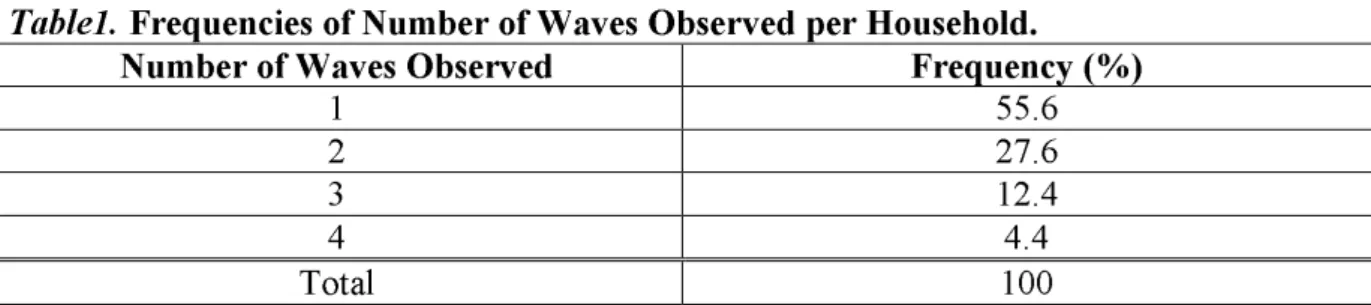
We use data from rounds V– VIII (1994-1998) of phase II as we will need the time use questionnaire to include household production in the empirical analysis. The sample used for the econometric analysis consists of couples where both partners are employed and the household head is of working age. That is, men are between 16 and 59 years old and both partners work. This yields an unbalanced panel of 1480 households (household heads) with 2419 observations, as some households are observed several times. After excluding households with missing values on key variables we are left with 2144 observations. Table 1 reports the percentage of households observed for 1, 2, 3 or 4 waves. More than half of households are observed only in one wave, and only 16.8% of households are observed more
than twice. Due to the small size of the panel, we pool the data and do not control for any invariant household effects in what follows. These effects can produce biases, but given the characteristics of the data these are expected to be insignificant. By contrast, we control for the period of observation in order to take into account common aggregate time-specific shocks due to the instability of the Russian economy during transition, and in particular instability in the Russian labor market.
Table1.
Frequencies of Number of Waves Observed per Household.
Number of Waves Observed
Frequency (%)
1 55.6
2 27.6
3 12.4
4 4.4
Total 100
Table 2 shows the sample means of the variables used in the econometric analysis.
Table 2.
Sample Means of Variables.
Women Men
Variable Round VIII
Means Round VII Means Round VI Means Round VIII Means Round VII Means Round VI Means Market time per
week (hi), hrs (15.38) 38.78 (14.68) 38.41 (12.23) 39.5 (17.25) 44.72 (16.84) 44.75 (12.99) 45.22 Domestic time per week (hhi), hrs 46.87 (29.8) (30.7) 45 (30.4) 42.9 (16.47) 14.72 (19.36) 15.71 (17.52) 13.74 Total working time per week (Hi), hrs 85.66 (31.92) (31.49) 83.23 (31.53)82.36 (22.69) 59.39 (24.93) 60.43 (22.48) 58.95 Hourly wage (wi), roubles (10.9) 3.87 (14.5) 6.12 (17) 7 (45) 7.8 10.46 (36) (55.5) 12.7 Household total monthly income (Y), roubles 2196 (14484) (5878) 2696 (6145) 2887 (14484) 2196 (5878) 2696 (6145) 2887
Source: RLMS. (standard errors in parentheses).
The difference in total working time between men and women is particularly striking: though women work slightly fewer hours in the market (as is the case in many countries), the total amount of domestic work performed by women is substantial, as is the difference between men’s and women’s total work hours.
2.2 Self-reported income and its interpretation
To measure individual income, we use the following Subjective Economic Ladder question from the RLMS: “Please imagine a 9-step ladder where on the bottom, the first step, stand the poorest people, and on the highest step, the ninth, stand the rich. On which step are you today?" We analyze the intra-family correlation in the answers to this question. Here we make the assumption that household members give the same answer to this question if they receive the same share (one half) of full household income, which includes monetary (market and domestic) as well as non-monetary income.
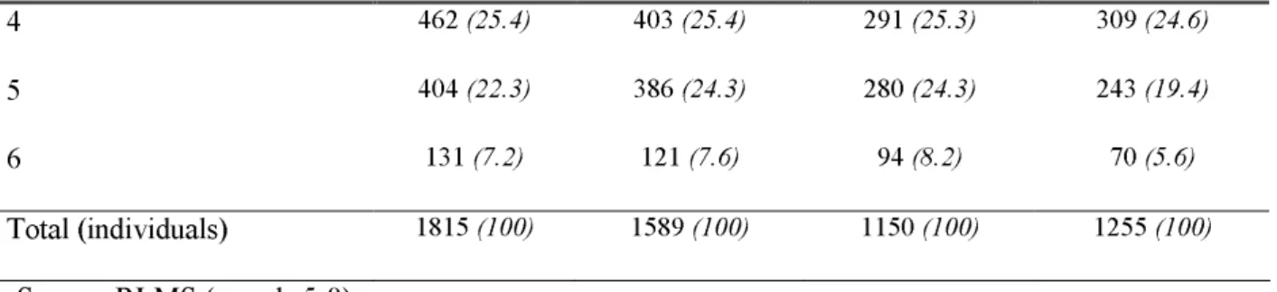
For the descriptive statistics we include all couples in which individuals both gave answers to the above question and provided wage information. To analyze self-rated income, we collapse the highest ranks (6, 7, 8, and 9) of the ladder into one category: few respondents considered themselves as amongst the richest. Table 3 summarizes the distribution of self-rated economic welfare. The vast majority of individuals feel poor: if we take the poorest two rungs to be the subjectively poor, the subjective poverty rate rose from 19.12% in 1994 to 23.91% in 1998. Most individuals say they are on steps 3, 4 and 5 of the 9-rung ladder.
Table 3.
Income Levels.
Economic Ladder Question 1- the poorest; 6 – the richest
Round 5 (1994) Number (%) Round 6 (1995) Number (%) Round 7 (1996) Number (%) Round 8 (1998) Number (%) 1 109 (6.0) 145 (9.1) 72 (6.3) 102 (8.1) 2 238 (13.1) 184 (11.6) 147 (12.8) 198 (15.8) 3 471 (25.9) 350 (22.0) 266 (23.1) 333 (26.5)
4 462 (25.4) 403 (25.4) 291 (25.3) 309 (24.6)
5 404 (22.3) 386 (24.3) 280 (24.3) 243 (19.4)
6 131 (7.2) 121 (7.6) 94 (8.2) 70 (5.6)
Total (individuals) 1815 (100) 1589 (100) 1150 (100) 1255 (100) Source: RLMS (rounds 5-8).
In this paper we are interested in income differences within a given household. Table 4 presents the differences in the Economic Ladder replies of husbands and wives. We consider married household heads, and compare their answer to that of their spouse. In over half of households men and women give different answers to the subjective question, as shown in Table 4. Almost 18% of men feel one step poorer than their wives and 10% differ by more than 2 steps. On average, women report lower incomes than men in the same households: in 1998, in over 34% of households the wife reports lower income, versus only 28% of households in which husbands reported being poorer. Our interpretation of the difference is that, as income sharing is the result of a bargaining process, income is not necessarily equally shared between husband and wife. This assumption is widely discussed and tested below.
Table 4.
Within household discrepancies in self-reported income
Wife’s score minus Husband’s score Round 5 (1994) Number (%) Round 6 (1995) Number (%) Round 7 1996) Number (%) Round 8 (1998) Number (%) -2 87 (10.8) 61 (9.4) 53 (11.3) 60 (11.8) -1 139 (17.3) 126 (19.4) 101 (21.6) 112 (22.1) 0 339 (42.2) 283 (43.5) 188 (40.3) 192 (37.9) 1 142 (17.7) 127 (19.5) 80 (17.1) 95 (18.7) 2 97 (12.1) 53 (8.1) 45 (9.6) 48 (9.5) Total households 804 (100) 650 (100) 467 (100) 507 (100)
Source: RLMS (rounds 5-8).
0- there is no difference between husband’s and wife’s responses. -1 – the wife is situated one step lower than her spouse, -2 –the wife is situated 2 or more steps lower than her spouse. 1- the wife is situated one step higher than her spouse, 2 – the wife is situated 2 or more steps higher than her spouse.
We use these income differences to construct an index of intra-household inequality for the empirical analysis.
2.3. Are subjective answers reliable?
We first provide some evidence to support the assumption that subjective data contain useful information. Ravallion and Lokshin (2001, 2002), for example, argue that though "the welfare inferences drawn from answers to subjective survey questions are clouded by concerns about measurement errors and how latent psychological factors influence observed respondent characteristics", subjective measures of income and poverty can be used as complements to standard socio-economic poverty measures. The use of subjective data, launched by the Leyden school in the 1970's for subjective poverty measurement, has developed rapidly since the late 1990's (Senik, 2005). Many nationally-representative household surveys such as the British Household Panel Survey (BHPS), the German Socio-Economic Panel (GSOEP) or the data used in this paper – the Russian Longitudinal Monitoring Survey (RLMS) – contain subjective questions related to general well-being, satisfaction with income, job, health and so on, or individuals' attitudes towards variables such as inequality or unemployment. These questions are generally used as proxies for welfare and well-being. In this reading, individuals themselves define their own level of welfare and provide information that would not be otherwise available, at least in large-scale surveys.
The main justification for the use of subjective data comes from the limitation of the axiom of revealed preferences (Senik, 2005). The traditional approaches to individual
behavior can be complemented by the use of data on individual perceptions in the cases when use of the former is restricted by the presence of externalities, social interactions, and so on. For example, subjective information is often used to reveal the non-pecuniary costs of unemployment (Clark and Oswald, 1994; Winkelmann and Winkelmann, 1998) and individuals' attitudes towards inequality can help to design redistributive policies (Ng, 1996; Ravallion and Lokshin, 2000). In general, these analyses provide consistent results that agree with our common sense. However, two key assumptions are necessary for the analysis of subjective data: that individuals are able to evaluate their own situation, and that responses can be compared between individuals (Ferrer-i-Carbonell, 2002). The reliability and validity of individual answers have been extensively studied in the recent literature (Diener, 1984; Diener et al., 1999; Veenhoven, 1993), and Easterlin (2001) has pointed out that "the general conclusion of such assessments is that subjective indicators,…, though not perfect, do reflect respondents' substantive feelings of well-being". Keeping these reflections in mind, we appeal to subjective data in a relatively new sphere: the analysis of intra-household inequality9.
A number of critics have worried about the comparison of income scales: people live in different social environments, so their answers about income may merely reflect their position relative to their own social environment rather than to a common scale. The argument is not totally convincing in our context, as we can assume that two individuals living together and sharing, at least partly, their income, have the same scale for self-positioning on the income ladder. We show below (Table 5) that both spouses have in mind an income including within household transfers when answering the question. Thus, for none of them would the often quoted reference group of work colleagues, for example, be relevant. Instead, here, the relevant reference group would rather be other households they know 9
As far as we know, the only other application of subjective information to intra-household distribution of welfare is Bonke and Browning (2003), in which they use a measure of self-perceived economic well-being).
(which could, of course, include colleagues of both sides). As husbands and wives share a similar social environment, they should thus share the same reference points regarding their income relative to that of other individuals in households that they know. Such reasoning is also supported by the finding of Plug and Van Praag (1998), who report that both adult partners appear to answer almost identically to subjective questions of the Leyden-type.
Another issue is that we may define equal sharing too narrowly. We are aware that interpreting small differences in the answers to subjective questions as revealing true inequality in income sharing may imply too high a level of confidence in interpersonal comparisons of subjective answers. We thus allow for some heterogeneity between partners by interpreting a difference of one in replies as indicating no difference in income (one being optimistic, the other one pessimistic, for example, or one being in an especially good mood on the day of the interview).
We construct an index which takes the value of 0 if the within household response difference equals -2 or less (the wife feels poorer than her husband); 1 if the difference between wife’s and husband’s replies is no greater than 1 in absolute value (the two partners report more or less the same income); and 2 if the wife reports higher economic welfare than her husband (a difference on the scale of at least 2)10.
A final objection concerns the question asked in the data: “on which step are you today?”. Although this is clearly asked on an individual basis within the individual questionnaire, it does not explicitly refer to household income-sharing. To test whether people, when answering this question, could have in mind their own earnings, rather than their share of household full income, we compute the simple correlations shown in table 5 below.
10We also ran the estimations with equal sharing corresponding to strict equality in the answers. The results were
Table 5
. Correlations between wages and household members’ replies to the income
question
Woman’s reply Man’s reply
wfhf 0.16 0.12
wmhm 0.18 0.23
Table 5 shows that household members clearly refer to a kind of household income, i.e. including within household transfers, rather than to their own earnings only when answering the income question. Couples agree that their income is more strongly correlated with the husband’s labor earnings (which generally contributes a larger share to total household monetary income), and more weakly correlated with the wife’s labor earnings (the wife’s monetary contribution being generally lower). Also note that, though a higher correlation is found for both with the husband’s earnings, the correlation with one own’s contribution to earnings is also found higher for both genders, than that given by the spouse for his/her spouse’s earnings. This is consistent with our interpretation in terms of a sharing rule. If a higher labor income increases my bargaining power, then, if my wage increases, I’ shall answer a higher value to the income question, for two reasons: first, because of a positive income effect, which exerts the same positive influence upon my spouses’ income, and, second, because of a “negotiation effect”, which increases my income share, but, conversely, decreases my spouse’s. Because of the negotiation effect, a stronger positive correlation is thus expected for each spouse with their own labor income than the correlation with the spouse’s labor income found for the opposite gender.
Having assumed that the data provide reliable information on the individual shares of full income, Φf and Φmwe can directly test the usual assumptions made regarding the
sharing rule.
The empirical model describing intra-household inequality (equation 1.4 above), can be formulated as an endogenous ordered probit, derived from the sharing rule. As the allocation of time is endogenous in this model, introducing household production requires that the profit from household production, Π, be endogenized. This is carried out here by adding two simultaneous equations of labor supply in domestic production, for husbands and wives. Note that, as the sharing rule itself is generally assumed to be a function of monetary characteristics (wages and non-labor income), but not directly of non-monetary variables, such as household productivity, the theoretical model implies that the only channel between the variables of the ordered probit and the two latter equations is via the profit from domestic production.
The model is estimated by full information maximum likelihood (FIML).
2.4.1 The econometric model
Let I be an index function taking values 0, 1 or 2 depending on whether the difference observed between female and male levels of income is negative, zero or positive.
0, if Φf <Φm
I= 1, if Φf =Φm (2.1)
2, if Φf >Φm
Let Φf * be a criterion function associated with an unobservable sharing rule: f
where Z is a vector of household-specific characteristics and distribution factors which are
assumed to influence the sharing rule. In particular, Z contains the difference in
wages(wm−wf) and non-labor income y. Note that here household exogenous income y can
be individualized, which also implies that individual exogenous incomes can be used as distribution factors.
The index function can then be written as: 0, if Φf *≤κ1,
I= 1, ifκ1 <Φf *≤κ2, (2.2)
2, if Φf *>κ2,
where k1 and k2 are unknown parameters to be estimated.
Recall that the sharing rule Φf depends on the profit from domestic production Π,
which is endogenous as household production depends on the time devoted to household work and wage rates. As such, system (2.2) needs to be completed by equations describing household work. The resulting system (2.3) is the econometric representation of the theoretical model (1.4): 0, if Φf *≤κ1, I= 1, if κ1 <Φf *≤κ2, 2, if Φf *>κ2, (2.3) and : tf = αfXf + u1 tm = αmXm + u2
where αi are the parameter vectors, Xi are the vectors of individual i specific characteristics and household-specific productivity factors. The error terms ε,u1andu2 are assumed to have
a trivariate standard normal distribution with zero mean and covariance matrix Σ:
1 σεu1 σεu2 Σ = 1 u ε σ 2 1 σ σu1u2 2 u ε σ σu1u2 σ22
with σεuj = cov (ε,uj), j=1, 2, σu1u2 = cov (u1,u2), σ12=Var(u ) 1 and σ22=Var(u ). 2
2.4.2 Maximum Likelihood Estimation
The model is estimated by full information maximum likelihood (FIML). This estimation method implements the full information ML procedure to estimate simultaneously the ordered and continuous parts of the model in order to provide consistent standard errors.
The likelihood function for the system of equations (2.3) is:
( )
(
)
[
]
∏
= × × − = 0 : 1 1 2 1 2 ) , ( , ' I i i i i i i i u u f u u F L κ γ Z ( )(
)
(
( ))
(
)
[
− − − ×]
× ×∏
=1 : 2 1 2 1 1 2 1 2 ) , ( , ' , ' I i i i i i i i i i u u f u u F u u F κ γ Z κ γ Z ( )(
)
[
]
∏
= × − − × 2 : 2 1 2 1 2 ) , ( , ' 1 I i i i i i i i u u f u u F κ γ Zwhere i denotes the ith observation, andF
(
.u1i,u2i)
is the conditional cumulative distributionThe variable εu1,u2 follows a normal distribution. Denoting = Σ ~ 2 1 σ σu1u2 2 1u u σ 2 2 σ
we can calculate its mean µ and variance σ² as follows (Greene, 2000):
( ) ( )
[
]
(
2)
1 1 2 2 2 1 2 2 2 1 1 1 2 1 1( , )' / / / / 1 ~ ) , (σ 1 σ 2 ρ σ ρ σ ρ ρ σ ρ σ ρ µ = ε ε Σ− u u = u + u − u + u − u u[
]
(
2)
2 1 2 2 2 1 1 2 1 ( , )~ ( , )' 1 2 1 2 1 2 1 σ σ σ ρ ρ ρρ ρ ρ σ σ = − εu εu Σ− εu εu = − + − − ,where ρ1, ρ2, and ρ are the coefficients of correlation between ε and u1, ε and u2, and u1 and u2 respectively.
The log of the likelihood function can be defined in terms of the cumulative standard normal distribution as below:
( )
∑
(
( ) ( )
)
∑
= × + = − × + = 1 : 1 2 1 0 2 0 0 : 1 2 1 0 ( , ) ln ( , ) ln ln I i i i i i I i F zi f ui u i F z F z f u u L( )
(
1)
( , ) ln 1 2 0 : 2 0 i i I i F zi f u u × − +∑
=with F0 standing for the cumulative standard normal distribution function and
σ µ) ' ( − − = j i i j i k z γ Z , (j=1, 2). 2.4.3. The results
The dependent variables are the natural logarithms of male and female monthly domestic labor supply in hours, and the index of intra-household inequality. All of the independent variables are here assumed to be exogenous. We include the wage rates of both husband and wife, individual demographic characteristics (age, age-squared and education),
household characteristics (number of children, assets and possession of durables) and type and region of settlement. The estimates are reported in Table 6 below.
Relatively few variables are significantly correlated with domestic labor supply. The partner’s wage rate is an important determinant of women’s domestic working time: higher male wages are associated with greater domestic labor supply by the wife, while higher female wages have no significant effect on males’ domestic work. Other significant variables in both equations are the number of young children (0-7 years old) and older children (7-18 years old) in the household: as expected, more children increase both spouses’ domestic work especially when the children are younger. Non labor-market variables are not significant here. Living space, durables possession or owning an individual plot do not influence the hours of domestic work of either husband or wife. Household work does vary by region and type of settlement. Both partners work less in Moscow and St-Petersburg, and in the Urals and Eastern and Western Siberia women's domestic labor supply is lower than in the other regions. As might be expected, both men and women living in rural areas work more at home than do those living in urban areas.
We have included in the ordered probit equation variables, such as non-labor income11, which we may expect to be correlated with the spouses’ bargaining power. As noted above, this index takes a value of 0 if the within household difference in replies is less than or equal to -2 (the wife feels poorer than her husband); 1 if this difference is no greater than 1 in absolute value (the two partners thus giving more or less the same answer to the income question); and 2 if the wife reports a higher level of income than her husband (with the difference on the scale being at least 2). The wage difference in these equations is expressed as the natural logarithm of the difference between female and male wages.
11 For each household, the data give information upon the different sources of income. Household non-labor
Table 6.
ML Estimation of Woman and Man's Domestic Labor Supply and the Index of
Intra-Household Inequality
a.
Woman's domestic labor supply Man's domesticlabor supply Index
a Marginal effects for the ordered probit
Coefficient Coefficient Coefficient dP(0)/dX3 dP(1)/dX3 dP(2)/dX3
Ln of man's wage rate 0.044*** 0.014 0.1*** 0.0007 -0.00004 -0.0006 Ln of woman's wage rate -0.006 0.015 -0.002 0.00011 0.002
Wage differenceb 0.17*** -0.022 0.0014 0.021
Man's age -0.014
Man's age squared 0.014
Woman's age 0.025**
Woman's age squared -0.026***
Age differencec -0.013** 0.002 -0.0001 -0.002
Woman has technical or higher education -0.032
Man has technical or higher education 0.054
Male education (years) -0.01 0.00004 -0.000003 -0.00003
Woman has higher degree of education than man 0.06 -0.015 0.03 -0.015 Household non-labor income -0.0002 -0.003 -0.0002 0.003 Number of children 0-7 years old 0.44*** 0.455*** 0.017 -0.011 -0.0007 0.01 Number of children 7-18 years old 0.19*** 0.171*** 0.06* -0.014 0.0008 0.013 Number of elderly persons in the household 0.021 0.121** 0.08 0.007 0.0004 -0.006 Ln of living space (sq. meters) -0.020 -0.063 -0.04 0.004 -0.0002 -0.003
Automobile owned 0.024 -0.053
Washing machine owned -0.030 0.003
Family is working on an individual plot 0.016 0.015 -0.02 0.004 -0.009 0.004
Rural 0.146** 0.22***
North Caucasian -0.030 0.03
Volga-Vaytski and Volga Basin -0.034 0.010
Moscow - St-Petersburg -0.09* -0.16** -0.02 -0.004 -0.008 0.004 Northern and North Western -0.072 0.135
The Urals -0.184** -0.06
Western Siberia -0.108* 0.01
Eastern Siberia and Far Eastern -0.15*** 0.034
Round 5 0.075* 0.162** 0.09 -0.02 0.04 -0.02 Round 6 0.006 0.019 0.044 -0.01 0.02 -0.01 Round 8 -0.06 -0.062 0.025 -0.006 0.011 -0.006 Constant 4.21*** 3.82*** Ancillary parameters k1 -1.2*** k2 1.34***
ρ1 (correlation between woman's domestic labor
supply and the sharing rule) -0.06* ρ2 (correlation between man's domestic labor
supply and the sharing rule) -0.03 ρ (correlation between man's and woman's supply) 0.27***
σ1 0.615***
σ2 0.985***
Number of observations 1916
Log likelihood -6462.59
* significant at the 10% level; ** significant at the 5% level; *** significant at the 1% level a The dependent variable is the index of intra household inequality: 0 – the wife reports being poorer than her husband; 1 – there is no difference, 2 – the wife reports being richer than her husband. b Wage difference: the difference between ln of woman's real wage rate and ln of man's real wage rate. c Age difference: the difference between woman's age and man's age
The reference categories are: Urban versus Rural, Central and Central Black-Earth for region, Round 7 for wave. Source: RLMS (rounds 5-8)
The results in Table 6 are in line with those predicted by the theory: the wage difference is highly significant with the "correct" sign.
We thus find, as expected, that the higher is the woman's wage compared to her husband’s, the greater is the probability that the woman's response to the income question is higher than her husband’s. This conclusion is confirmed by the marginal effects analysis in the right-hand panel of Table 6. The marginal effects are almost the same in absolute value for the first and third categories of the dependent variable, so the result is symmetric. The wage ratio is therefore a powerful determinant of the outcome of intra-household bargaining. Another variable which influences the distribution of full income among household members is the age difference, here the wife's age minus her husband's age. The estimated coefficient on this variable is negative and significant: the older the woman is relative to her husband, the lower the probability of the woman's higher response. The effect of the age difference can be interpreted as showing the greater bargaining power of women who are relatively younger compared to their husband. On the other hand, we find no significant effect of the difference in partners’ education levels on the distribution of income within the household.
These results are in accordance with the collective model predictions and strongly support the assumption made throughout the paper that the answers given to the income question do correspond to individual income shares, which themselves are the result of a bargaining process. Note that in the case of the unitary model of household behaviour, the total individual income of each partner would be the same and the discrepancies in self reported levels would be random and thus not related to the wages or to age differences as it is found here.
The correlations between domestic labor supplies and the sharing rule are low (see Table A1 in the Appendix for the values of ρ1 and ρ2). This result provides some support for our further assumption that the surplus from domestic production (profit Π in the theoretical
model) is negligible compared to other sources of household income. This is equivalent to assuming that household production is evaluated at its market price, i.e. using the level of wages.
The results of our estimation show that the wage and age differentials are important determinants of intra-household inequality. These results support the choice of the collective model to analyze the intra-household allocation of income.
We now turn to the second main objective of the paper, namely the identification of the sharing rule.
3. IDENTIFYING THE SHARING RULE: A NEW METHOD
Rapoport, Sofer and Solaz (2003) show that, if the allocations of household members’ time between domestic work, market work and leisure are observable, and if there exists at least one observable distribution factor, then the sharing rule can be recovered up to a constant.
Here, additional information on the income levels of household members provides us with a supplementary constraint allowing to completely identifying the sharing rule.
The derivatives of the sharing rule can be computed using the estimated parameters of the simultaneous estimation of total labor supply (market plus domestic work):
Hf =
β
fQ
+ v1 (3.1)Hm =
β
mQ
+ v2 with Hi = hi + ti,i = f,mwhere
β
i are the parameter vectors,Q
=(wf,wm,yf,ym,s,z) is a vector whose componentsare the individuals’ specific characteristics and household-specific distribution factors, and v1 and v2 are distributed bivariate normally. We call this result R1
The next step is to identify the constant of the sharing rule, as well as its derivatives12. To do this, assume that Π is observable (which is not the case), Φf (wf,wm,yf,ym,s,z) can
be recovered from the sample of households who share full income (approximately) equally. For this sample, we have:
f
Φ = Φm =12
[
(wm+wf)T+ y+Π]
(3.2)Unfortunately, Π never can be observed. We thus assume in addition that, empirically, the surplus from domestic production is negligible compared to other sources of household income. This is equivalent to assuming that household production is evaluated at its market costs, i.e. wages.
The empirical justification for this assumption is the low values found for the correlations between domestic labor supply and the sharing rule equations (ρ1 and ρ2 in equations (2.3) above). The correlation between men’s hours of domestic work and the index of intra-household inequality is negative, small (-0.03) and insignificant. For women, the correlation is also small, negative (-0.06) but significant at the 10% level. As, for households where both members participate in the labor market, Π is the only channel in the theoretical model through which domestic work and the sharing rule could be correlated, these findings support the assumption that we make above.
Here, we propose a direct identification method, based on the additional condition provided by the index of intra-household equality. For this, we use a two-stage estimation.
12 Note that Rapoport, Solaz and Sofer, 2005, gives a method for estimating the derivatives of the sharing rule
3.1 A Two-stage estimation approach
In theory, the estimation of the total labor supplies of the two household members on the sub-sample of the couples for whom full income shares are fully “observed” should allow us to identify the individual shares of full income for the rest of the sample. One problem, we face, though, is that of over-identification: the estimates of individual full income shares should sum up to the (observed) full income, which is generally not the case. We thus chose the strategy of estimating rather the ratio of full income shares. We use three equations:
+ + Φ + = + + Φ + = m m m m m m m f f f f f f f e H e H X γ X γ ln ln β α β α (3.6) and λ + = Φ Φ δX f m ln , (3.7)
where (αf,αm,βf,βm),γf,γm,δ are the parameter vectors; Xf and Xm are respectively the
vectors of female and male individual characteristics; X=(wf,wm,yf,ym,s,z); e ,f em and
λ are the error terms which are assumed to have a joint normal distribution with zero means. To this we add the budget constraint: Φ=Φf +Φm =(wf +wm)T+ y
Using the sub-sample S1 of households who are assumed to share full income equally,
i.e. here the sub-sample of couples for whom the index value calculated above is 1 (the same
answer, plus or minus one, to the subjective ladder question), we obtain:
m
f =Φ
Φ =
[
(wm +wf)T +y+Π]
2 1
Or, assuming Π to be only small, m f =Φ Φ =
[
(wm +wf)T +y]
2 1 (3.8)The system (3.6) can then be estimated using this sub-sample.
In this first stage the vectors of parameters (αf,αm,βf,βm),γ ,f γm can be identified.
Note that the probability mass corresponding to the index value of 1 is continuously spread over the interval
[
Φ*f −k1;Φ*f −k2]
rather than being concentrated at the pointm
f =Φ
Φ =1 2
[
(wm +wf)T+ y]
. Thus for those individuals belonging to the sub-sample S1 the hypothesized equality between partners’ full incomes holds only approximately: we have made this choice (see section 2 above) in order to make our formal definition of equality at the same time less restrictive and more realistic. According to our interpretation, our measures of Φf and Φm as 12[
(wm +wf)T +y]
are subject to error, implying that the estimators arebiased towards zero (Greene, 2000). This bias can be corrected by using the results obtained from the ordered probit model.13
Another source of bias is sample selection when we use the sub-sample of couples for whom the index value is 1. We correct for this selection bias by using the results from the ordered probit model. The method and demonstration are contained in Appendix A.
The vector of parameters δ is identified in the second stage by estimating (3.7) and using the whole sample of households.
lnRˆ =δX+i (3.9)
where lnRˆ is the predicted logarithm of the ratio between the man’s and the woman’s shares:
f f f f f m m m m m H H R lnˆ =( −α −γ X )⋅β −( −α −γ X )⋅β (3.10)
and the error term i follows a normal distribution with zero mean:
f f m m e e i=λ+ /β − /β
Finally the shares Φf and Φm are calculated using the predicted sharing ratio
f m R Φ Φ = ˆ and
their sum equalized to (observed) full income: Φ=Φf +Φm =(wf +wm)T +y.
Due to the poor quality of our measure of non-labor income, which cannot be individualized correctly in the RLMS data, the latter strategy is followed in the empirical analysis. The method of estimation is 3SLS in the first stage and OLS in the second stage.
3.2. The estimation results
3.2.1. Labor Supply Estimations
The explanatory variables used in the total labor supply estimations (market plus domestic work) are the natural logarithm of the individual’s full income calculated using (3.8), individual characteristics (age, age squared, number of years of education), household characteristics (number of children, presence of elderly persons, possession of durables such as a car, a washing machine etc.), and type and region of housing.
The dependent variable in the sharing rule equation is the predicted ratio between the male and female shares of full income, Rˆ. The vector of explanatory variables includes the
natural logarithms of the wage rates and their squares, and the same individual and household characteristics as in section 2. The estimates are reported in Table B (Appendix B).
The main results are as follows. The total labor supply of both household members is positively correlated with their individual full incomes and is negatively correlated with their wage rates. This implies a negative relationship between (true) leisure and wages, which, in turn, can be interpreted as incomes being so low that leisure is a very expensive good: the substitution effect dominates the income effect.
3.2.2. Restrictions on the Slutsky Matrix
The Slutsky condition for the labor supply model implies that the wage response of the compensated supply of labor is non-negative:
0 ≥ ∂ ∂ i c i w H or 0 ln ) ( ln ∂ Φ ≥ ∂ − Φ + ∂ ∂ i i i i i i i Hw T H H w
Given the outcomes of the coefficients estimates in Table C (Appendix C), the latter condition is satisfied for both female and male labor supply for the whole sample of observations as well as at the mean wages, labor supply and full incomes.
3.2.3. Sharing Rule Estimation
Due to the nonlinearity of the estimated equation in terms of wages, the elasticity of the dependent variable with respect to wages is defined by both a constant term and a term
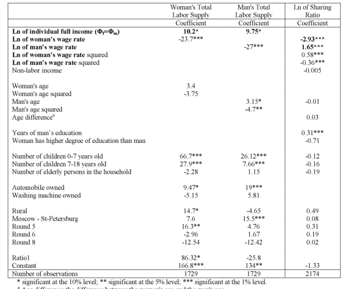
which depends on the corresponding wage14. The constant term of the sharing ratio elasticity with respect to wages is in each case large and significant: -2.93 for women’s wages and 1.65 for men’s. That is, the direct effect of women’s wages on the sharing ratio is negative, so that the effect of women’s wages on the woman’s share is positive, and negative on the men’s share. Symmetrically, the direct effect of men’s wages on the sharing ratio is positive, so that the effect of male wages on the woman’s share is negative, and the effect on the man’s share is positive. The direct effect of women’s wages is stronger than that of men’s wages. This finding is consistent with the presence of intra-household bargaining. The elasticities of the sharing ratio with respect to both wages calculated at their mean level, are given in Table 7. This table also includes the effect of non-labor income and various household characteristics, allowing us to compare the size of the effect of the different variables on income sharing. R
refers to the sharing ratio of full income: R = Φm/Φf.
The effect of non-labor income is small and insignificant. However, this result is not totally convincing due to the poor quality of the non-labor income variable. The sharing ratio increases with the man’s education and is sharply lower if the woman’s level of education is higher than her husband’s (although then the latter effect is not significant). Hence, differences in education have a large impact on full-income sharing in the household. The number of children and of elderly people has a negative impact on this ratio, and hence exerts a positive effect on the woman’s share but these effects are not significant.
Table 7.
Marginal Effects of Wage Rates and other Explanatory Variables on the
Sharing Rule (R).
14 i w k k w R ln ln ln 2 1+ = ∂ ∂ , i = f, m; where kMarginal Effect
(in roubles). ∂lnR/∂lnwf -0.33*** ∂lnR/∂lnwm -0.13*** ∂R/∂wf -0.2*** ∂R/∂wm -0.005*** ∂R/y 0 ∂R/∂(Man's age) -0.01 ∂R/∂(Agef– Agem) 0.02∂R/∂(Years of man’s education) 0.3***
∂R/∂(Woman has higher degree) -0.6
∂R/∂(Number of children 0-7 years old) -0.18
∂R/∂( Number of children 7-18 years old) -0.13
∂R/∂( Number of elderly persons in the household) -0.52
* significant at the 10% level; ** significant at the 5% level; *** significant at the 1% level.
The elasticity as well as the marginal effects of wages show that, at mean wages, the sharing ratio falls when the wages of both household members increases. The effect is much stronger, though, for women’s wages than for men’s. That is, a raise in any wage benefits women more than it does men. However, this effect is much stronger in the case of an increase in the woman’s own wages than for an increase in male wages.
3.2.1. Simulating the sharing rule
The results above can be summarized by a numerical example. Consider an average Russian household, represented by a 39-year old woman earning 8 roubles per hour, whose husband is 41 years old earning 13 roubles per hour. Assume that they have a 7-year old child (or older), that both received 13 years of education, that the family lives in a city in the Urals, and that the wave chosen for this exercise is round 7. The variables used in these calculations for the shares and transfers refer to monthly incomes.
The model yields an estimated probability of 79% that husband and wife report equality in the sharing of income as measured by our index, I, with the full incomes of the household members amounting to 10920 roubles for the woman and 13156 for the man.
Now assume that woman’s wages are the same as her husband’s. The probability that the wife receives a lower share decreases to 10 % and predicted income sharing approaches equality, with a ratio between shares of 1.06.
A one rouble increase in the woman’s wage rate leads to a slightly less unequal sharing of household full income, with 11344 roubles allocated to the wife and 13404 allocated to the husband. A one rouble increase in the man’s wage rate leads to equal sharing of the extra income (about 335 roubles for each partner) with consequently a slightly less unequal sharing of full income (11258 for the woman and 13490 for the man).
Assume now that the family has another child, aged between 7 and 18, then the probability of the wife receiving a larger share increases to 10.4% and full income would be reallocated with about 1000 roubles passing from husband to wife. The same reallocation is predicted if the second child is younger or is replaced by an elderly person. Therefore, the presence of children and of elderly persons increases the woman’s bargaining power.
The wife’s education being higher than her husband’s (for example higher education versus technical studies) has a strong effect on the sharing of full income, with the woman now receiving 60%.
The impacts of these various changes on the sharing rule are summarized in Table 8 below.
Table 8.
Predicted Impact of Various Changes in the Covariates on the Probability of
Equal Full Income Sharing and on the Shares of the Two Partners
P0
∆
wf = 1 rouble 11344 13404 1.18 424 247∆
wm = 1 rouble 11258 13490 1.198 337 334∆
wf = wf - wm 10 79 11 13608 14499 1.06 2688 1343A second
younger child
10 79 11 11623 12453 1.07 703 -703A second older
child
9.6 79 11.4 11887 12189 1.03 967 -967An elderly
person
12 79 9 12063 12012 1 1143 -1143Woman’s
higher degree
9.5 82 8.5 15097 8978 0.6 4177 -4177P0
: Probability of the index taking a value of 0 (wife reports being poorer)P1
: Probability of the index taking a value of 1 (equality)P2
: Probability of the index taking a value of 2 (wife reports being richer)∆
Φf: Change in woman’s share.∆
Φm: Change in man’s share.∆
wf: Woman’s wage rate change with respect to the control value∆
wm: Man’s wage rate change with respect to the control valueCONCLUDING REMARKS
In this paper we have proposed an application of the collective model to the analysis of intra-household inequality using self-reported income scales. We use a collective model taking into account household production. The results support the assumptions of the collective model. The wage difference within the household is found to be a strong determinant of the intra-household sharing of resources.
We then set out a new method of identification of the sharing rule. Using the results obtained from couples who report the same level of income, and interpreting this as equal income-sharing, we are able to identify the sharing rule for the whole sample. The results are consistent with those predicted by the model: as expected, wages and education level exert a strong influence on the sharing rule, with an increase in female wages increasing women’s share more strongly than does an increase in male wages. Perhaps more unexpected is the positive effect of children and of elderly persons on the wife’s share. This seems to indicate that variables other than those related to market wages or non-labor income can influence
intra-household bargaining. Exploring this result further should be the aim of future research, from both an empirical as well as a theoretical point of view.
REFERENCES
APPS, PATRICIA F., and REES, RAY (1997) "Collective Labor Supply and Household Production", Journal of Political Economy, 105, pp. 178-190.
BONKE, J. AND BROWNING, M. (2003), "The distribution of well-being and income within the household", University of Copenhagen. Department of Economics, Centre for Applied Microeconometrics Working Paper n° 2003-01.
BOURGUIGNON, F. and CHIURI, M.C. (2005), “Labor Market Time and Home Production: a new test for collective models of intra-household allocation”, CSEF Working Paper 131. BROWNING, M. and CHIAPPORI, P-A. (1998) "Efficient Intra-Household Allocations: A
General Characterization and Empirical Tests", Econometrica, 66, pp. 1241-1278.
BROWNING, M., CHIAPPORI, P-A. and LEWBEL, A. (2004) "Estimating Consumption Economies of Scale, Adult Equivalence Scales, and Household Bargaining Power",
mimeo.
CHIAPPORI, PIERRE-ANDRÉ (1998) "Rational Household Labor Supply", Econometrica, 56, pp. 63-89.
CHIAPPORI, PIERRE-ANDRÉ (1992) "Collective Labor Supply and Welfare", Journal of Political Economy, 100, pp. 437-467.
CHIAPPORI, PIERRE-ANDRÉ (1997) "Introducing Household Production in Collective Models of Labor Supply", Journal of Political Economy, 105, pp. 191-209.
CHIAPPORI, P-A., FORTIN, B. and LACROIX, G. (2002) "Marriage Market, Divorce Legislation and Household Labor Supply", Journal of Political Economy, 110, pp.37-72.
CLARK, A.E., and OSWALD, A.J. (1994). "Unhappiness and Unemployment". Economic Journal, 104, 648-659.
DIENER, E. (1984) "Subjective wellbeing”. Psychological Bulletin, 93, pp. 542-575;
DIENER, E., E.M. SUH, R.E. LUCAS and H.L. SMITH (1999) "Subjective wellbeing: Three decades of progress", Psychological Bulletin, 125, pp. 276-302;
EASTERLIN, R.A. (2001) "Income and Happiness: Towards a Unified Theory", Economic Journal, 111(July), pp.465-484;
FERRER-I-CARBONELL, A. "Subjective Questions to Measure Welfare and Well-being",
Tinbergen Institute Discussion Paper, 2002-020/3.
FERRER-I-CARBONELL, A. and FRIJTERS, P. (2004) "How important is methodology for the Estimates of the determinants of happiness?", Economic Journal, July, pp. 641-659. GREENE, W. H.(2000), Econometric Analysis, Fourth Edn., Englewood Cliffs, Prentice-Hall. NG, Y-K. (1996) "Happiness surveys: Some comparability issues and an exploratory survey
based on just perceivable increments", Social Indicators Research, 38(1), pp.1-27;
PLUG, E.J.S., VAN PRAAG, B.M.S. (1998), "Similarity in response behavior between household members: An application to income evaluation". Journal of Economic Psychology, 19, 497- 513.
RAPOPORT, B., SOFER, C., and SOLAZ, A. (2003), “Household Production in a Collective Model: Some New Results”, TEAM Working Paper, Université Paris 1-Panthéon-Sorbonne.
RAPOPORT, B., SOFER, C., and SOLAZ, A. (2005), “La production domestique dans les modèles collectives", Actualité Economique, forthcoming;
RAVALLION, M. and LOKSHIN, M. (2000) "Who wants to redistribute? The tunnel effect in 1990s Russia", Journal of Public Economics, 76, pp.87-104
RAVALLION, M. and LOKSHIN, M. (2001) "Identifying Welfare Effects from Subjective Questions", Economica, N°68, pp. 335-357.
RAVALLION, M. and LOKSHIN, M. (2002) "Self-Rated Economic Welfare in Russia",
European Economic Review, N°46, pp. 1453-1473.
SENIK, C. (2004) “When Information Dominates Comparison. Learning from Russian Subjective Panel Data”, Journal of Public Economics, 88, p. 2099-2133.
SENIK, C. (2005) "What Can we Learn from Subjective Data? The Case of Income and Well-Being", Journal of Economic Surveys, 19 (1), pp. 43-63.
VEENHOVEN, R. (1993). Happiness in Nations, Subjective Appreciation of Life in 56 Nations 1946-1992. Rotterdam: Erasmus University.
WINKELMANN, L. and WINKELMANN, R. (1998) "Why are the Unemployed So Unhappy? Evidence from Panel Data", Economica, 65, pp. 1-15.
APPENDIX A
The correction term Ratio1 of the selection bias in the labor supply equations is constructed as follows: ) = | = ) = | ) = = 1) E (E(e | ε Ι 1 M1(σ )E(ε Ι 1 | I E(ei i eiε ,
where M2(σeiε) is a coefficient depending on the covariance between ε and ei to be estimated,
i = 1,2. Ratio1 = ) ( ) ( ) ( ) ( 1 1 2 12 21 z F z F z f z f z ε z (ε E Ι (ε E − − = ) < < | = ) = | ,
APPENDIX B
Table B.
3SLS Estimation of Woman’s and Man's Total Labor Supply and Sharing
Ratio.
Woman's Total
Labor Supply Labor Supply Man's Total Ln of Sharing Ratio Coefficient Coefficient Coefficient
Ln of individual full income (Φf=Φm) 10.2* 9.75*
Ln of woman's wage rate -23.7*** -2.93***
Ln of man's wage rate -27*** 1.65***
Ln of woman's wage rate squared 0.58***
Ln of man's wage rate squared -0.36***
Non-labor income -0.005
Woman's age 3.4
Woman's age squared -3.75
Man's age 3.15* -0.01
Man's age squared -4.7**
Age differencea 0.03
Years of man’s education 0.31***
Woman has higher degree of education than man -0.71 Number of children 0-7 years old 66.7*** 26.12*** -0.12 Number of children 7-18 years old 27.9*** 7.66*** -0.16 Number of elderly persons in the household -2.28 1.15 -0.19
Automobile owned 9.47* 19***
Washing machine owned -5.15 5.81
Rural 14.7* -4.65 0.49 Moscow - St-Petersburg 7.6 15.5*** 0.08 Round 5 16.3** 4.76 0.31 Round 6 -2.96 1.67 0.19 Round 8 -12.54 -12.42 0.02 Ratio1 86.32* -25.8 Constant 166.8*** 134** -1.33 Number of observations 1729 1729 2174
* significant at the 10% level; ** significant at the 5% level; *** significant at the 1% level. a Age difference: the difference between the woman's age and the man's age.
The reference categories are: Urban versus Rural, region other than Moscow and St Petersburg, Round 7 for round of observation.