HAL Id: hal-02968755
https://hal.archives-ouvertes.fr/hal-02968755
Submitted on 19 Oct 2020
HAL is a multi-disciplinary open access
archive for the deposit and dissemination of
sci-entific research documents, whether they are
pub-lished or not. The documents may come from
teaching and research institutions in France or
abroad, or from public or private research centers.
L’archive ouverte pluridisciplinaire HAL, est
destinée au dépôt et à la diffusion de documents
scientifiques de niveau recherche, publiés ou non,
émanant des établissements d’enseignement et de
recherche français ou étrangers, des laboratoires
publics ou privés.
William Gray, Robert Wills, James Rae, Andrea Burke, Ruza Ivanovic,
William Roberts, David Ferreira, Paul Valdes
To cite this version:
William Gray, Robert Wills, James Rae, Andrea Burke, Ruza Ivanovic, et al.. Wind-Driven
Evolu-tion of the North Pacific Subpolar Gyre Over the Last DeglaciaEvolu-tion. Geophysical Research Letters,
American Geophysical Union, 2020, 47 (6), �10.1029/2019GL086328�. �hal-02968755�
William R. Gray1,2 , Robert C. J. Wills3 , James W. B. Rae2 , Andrea Burke2 , Ruza F. Ivanovic4 , William H. G. Roberts5 , David Ferreira6 , and Paul J. Valdes7
1Laboratoire des Sciences du Climat et de l'Environnement (LSCE/IPSL), Université Paris‐Saclay, Université Paris-Saclay,
Gif‐sur‐Yvette, France,2School of Earth and Environmental Science, University of St Andrews, Saint Andrews, UK, 3Department of Atmospheric Sciences, University of Washington, Seattle, WA, USA,4School of Earth and Environment,
University of Leeds, Leeds, UK,5Geography and Environmental Sciences, Northumbria University, Newcastle, UK, 6Department of Meteorology, University of Reading, Reading, UK,7School of Geographical Sciences, University of Bristol,
Bristol, UK
Abstract
North Pacific atmospheric and oceanic circulations are key missing pieces in our understanding of the reorganization of the global climate system since the Last Glacial Maximum. Here, using a basin‐wide compilation of planktic foraminiferal δ18O, we show that the North Pacific subpolar gyre extended ~3° further south during the Last Glacial Maximum, consistent with sea surface temperature and productivity proxy data. Climate models indicate that the expansion of the subpolar gyre was associated with a substantial gyre strengthening, and that these gyre circulation changes were driven by asouthward shift of the midlatitude westerlies and increased wind stress from the polar easterlies. Using single‐forcing model runs, we show that these atmospheric circulation changes are a nonlinear response to ice sheet topography/albedo and CO2. Our reconstruction indicates that the gyre boundary (and thus
westerly winds) began to migrate northward at ~16.5 ka, driving changes in ocean heat transport, biogeochemistry, and North American hydroclimate.
Plain language summary
Despite the North Pacific's importance in the global climate system, changes in the circulation of this region since the last ice age are poorly understood. Today, the North Pacific Ocean has distinct properties north and south of ~40°N: To the south, the warm surface waters form a circulation cell that moves clockwise (the subtropical gyre); to the north, the cold surface waters form a circulation cell that moves anticlockwise (the subpolar gyre). This difference in surface ocean circulation north and south of ~40°N is determined by the wind patterns. Here, using a compilation of oxygen isotopes measured in the carbonate shells of fossil plankton from sediment cores across the basin, which tracks changes in the spatial pattern of temperature, we reconstruct how the position of the boundary between the gyres changed since the last ice age. Our results show that the boundary between the gyres was shifted southward by ~3° during the last ice age; this indicates that the westerly winds were also shifted southward at this time. Using numerical simulations of the climate, wefind that this ice age shift in the westerly winds is primarily due to the presence of a large ice sheet over North America.1. Introduction
Despite the North Pacific's importance in the global climate system, the reorganization of the atmosphere and surface ocean in this region during the Last Glacial Maximum (LGM, ~20 ka) and the last deglaciation (~10–20 ka, “the deglaciation” from here on) remains poorly constrained. Changes in atmospheric and near‐surface ocean circulation within the North Pacific are potentially important drivers of observed changes in the overturning circulation and biogeochemistry of the North Pacific during the LGM and deglaciation, suggested to play a role in regulating atmospheric CO2(Gray et al., 2018; Keigwin, 1998;
Okazaki et al., 2010; Rae et al., 2014). The overturning and gyre circulations are also important influences on poleward ocean heat transport.
Large changes in the hydroclimate of western North America during the LGM and the deglaciation (e.g., Ibarra et al., 2014; Kirby et al., 2013; Lyle et al., 2012; McGee et al., 2012; Nelson et al., 2005; Oviatt et al., 1999) have been suggested to result from the reorganization of North Pacific atmospheric circulation (e.g.,
©2020. American Geophysical Union. All Rights Reserved.
Key Points:
• Planktic foraminiferal δ18O data indicate that the North Pacific subpolar gyre expanded southward by ~3° during the Last Glacial Maximum
• Climate models show that changes in gyre extent/strength are driven by a nonlinear response of the westerlies to ice sheet albedo/topography and CO2 • Proxy data and model simulations
indicate that the gyre boundary and westerlies began to migrate northward at ~16.5 ka, during Heinrich Stadial 1 Supporting Information: • Supporting Information S1 • Table S1 • Data Set S1 • Figure S1 Correspondence to: W. R. Gray, william.gray@lsce.ipsl.fr Citation:
Gray, W. R., Wills, R. C. J., Rae, J. W. B., Burke, A., Ivanovic, R. F., Roberts, W. H. G., et al. (2020). Wind‐driven evolution of the North Pacific subpolar gyre over the last deglaciation. Geophysical Research Letters, 47, e2019GL086328. https://doi.org/ 10.1029/2019GL086328
Received 22 NOV 2019 Accepted 24 FEB 2020
Lora, 2018; Lora et al., 2017; Oster et al., 2015; Wong et al., 2016), with early modeling work suggesting a southward displacement of the westerly jet with the presence of the Laurentide Ice Sheet (Bartlein et al., 1998; Manabe & Broccoli, 1985). However, evidence for this atmospheric reorganization has not yet been identified in marine records.
Driven by opposite signs in the climatological wind stress curl (∇ × τ), the subtropical and subpolar gyres of the North Pacific Ocean have vastly different physical and chemical properties (Boyer et al., 2013; Key et al., 2015). The boundary between the gyres (defined as the point between the gyres at which the barotropic stream function [Ψbarotropic] = 0) is determined by Sverdrup balance and occurs where∇ × τ integrated from the eastern boundary
of the basin is 0 (Deser et al., 1999; Sverdrup, 1947). Today, the gyre boundary (which broadly determines the posi-tion of the subarctic front) is nearly zonal and lies at ~40°N, approximately following the local∇×τ = 0 line. South of ~40°N, anticyclonic wind stress curl in the subtropical gyre (STG) results in surface convergence and Ekman pumping (downwelling), allowing warm, nutrient‐poor, surface waters to accumulate. North of ~40°N, cyclonic wind stress curl in the subpolar gyre (SPG) results in surface divergence and Ekman suction (upwelling), bringing cold, nutrient‐rich, waters from the oceans interior to the surface. Surface ocean chlorophyll concentrations are an order of magnitude higher in the SPG than in the STG. The gyre circulation also dominates ocean heat transport in the Pacific (Forget & Ferreira, 2019). The relative extent and the strength of the gyres therefore exert a large influence over basin‐wide ecology, biogeochemistry, and climate.
Coupled climate models predict an ~60% increase in wind stress curl within the subpolar North Pacific under glacial forcings compared to preindustrial forcings (Gray et al., 2018). By Sverdrup balance (Sverdrup, 1947), this should result in a large and predictable response in the gyre circulation. Despite some early work sug-gesting that the subarctic front may have shifted southward during glacial times (Sawada & Handa, 1998; Thompson & Shackleton, 1980), little is known about gyre circulation over the deglaciation. Here, we use meridional profiles of planktic foraminiferal δ18O to reconstruct the position of the gyre boundary over the deglaciation. Given the relatively simple dynamical link between gyre circulation and wind stress, our gyre boundary reconstruction also helps constrain the deglacial reorganization of the atmospheric circula-tion. We use an ensemble of climate models forced by a range of boundary conditions to further explore the causes and implications of our gyre boundary reconstruction for the atmospheric and near‐surface ocean circulations within the North Pacific.
2. Methods
2.1. δ18O as a Tracer of Gyre Circulation
Theδ18O of planktic foraminiferal calcite (δ18Ocalcite) is a function of both theδ18O of seawater (δ18Owater)
and temperature dependent fractionation (δ18Ocalcite‐water; supporting information); however, at the basin
scale the effect of temperature is far greater than the effect ofδ18Owater. The large (~20 °C) sea surface
tem-perature (SST) difference between the gyres (Boyer et al., 2013) drives a calcite‐water fractionation that is ~5.5‰ greater in the SPG than in the STG (Figure 1d; supporting information). Therefore, although the δ18O of seawater is ~1‰ lighter in the SPG compared to the STG due to its lower salinity (~1.5 PSU,
Boyer et al., 2013; Figure 1c),δ18Ocalciteis ~4.5‰ higher in the SPG than the STG (Figure 1e). The two gyres
are thus clearly delineated in theδ18O of planktic foraminiferal calcite predicted using modern temperature and δ18Owater (Figure 1e), with the steepest meridional gradient in δ18Ocalcite at the gyre boundary
(Figure 1f). The meridional profiles of SST and thus δ18
Ocalciteare set by the gyre circulation (Yuan &
Talley, 1996; Figure S1), allowing us to use meridional profiles of planktic foraminiferal δ18Ocalciteto identify
the gyre boundary. While there are likely to be localδ18Owaterchanges across the basin over the deglaciation,
a salinity difference of ~12.5 PSU (using the North Pacific salinity‐δ18Owaterrelationship from LeGrande &
Schmidt, 2006) would be required to overcome the temperature signal between the gyres. As no mechanism exists to drive such a salinity/δ18Owaterdifference, temperature will always dominate the meridional pattern
ofδ18Ocalcite(Figure 1f) and we can use meridional profiles of δ18Ocalciteto track the position of the gyre
boundary through time.
We compiled previously published planktic foraminiferalδ18Ocalciterecords from near‐surface dwelling
spe-cies G. ruber, G. bulloides, and N. pachyderma, spanning the last deglaciation from the North Pacific Ocean (Figure 1; supporting information). The gyre boundary is clearly defined by the steepest meridional gradient
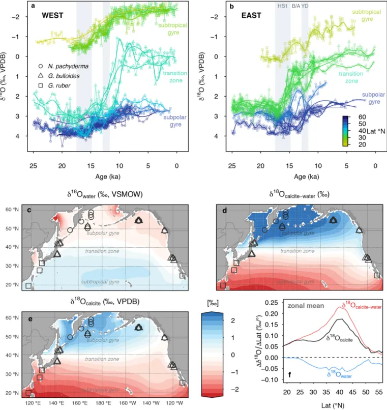
Figure 1. Planktic foraminiferalδ18O versus age with core site latitude represented by color. Data are divided east (b) and west (a) of 180°. HS1, B/A, and YD are Heinrich Stadial 1 (14.8–17.5 ka), Bølling‐Allerød (12.9–14.8 ka), and the Younger Dryas (11.8–12.9 ka), respectively. (c) Gridded δ18Owaterfrom LeGrande and
Schmidt (2006). (d) Calcite‐water fractionation calculated using WOA13 mean annual temperature (Boyer et al., 2013) and the temperature‐fractionation relationship of Kim and O'Neil (1997). (e) Predictedδ18Ocalciteusing griddedδ18Owaterfrom LeGrande and Schmidt (2006) and calcite‐water fractionation calculated using WOA13 mean annual temperature (Boyer et al., 2013) and the temperature‐fractionation relationship of Kim and O'Neil (1997) (note that the color scale is the same for all three panels). (f) Slope of the zonal mean meridional gradient inδ18Owater,δ18Ocalcite‐water, andδ18Ocalcite, as shown in (c), (d), and (e).
(Δδ18Ocalcite/ΔLatitude) in the Holocene planktic foraminiferal δ18Ocalcite data (Figure 2; supporting
information). The difference in meridional temperature gradient between the east and west of the basin is also evident in the Holoceneδ18Ocalcitedata, with a steeper gradient in the west of the basin (Figure 2b).
To reconstruct the position the of gyre boundary over the deglaciation, wefirst model the δ18Ocalcitedata as a
function of latitude, using a generalized additive model (GAM) in the mgcv package in R (Simpson, 2018; Wood, 2011; Wood et al., 2016) at 100 yr time steps from 18.5 to 10.5 ka (supporting information; Figures S2–S4). The smoothing term was calculated using restricted maximum likelihood (Reiss & Ogden, 2009; Wood et al., 2016). We then calculate the change in gyre boundary position over the deglaciation as the latitudinal shift (x°) that minimizes the Euclidean distance (L2) between the Holocene (taken as 10.5 ± 0.5 ka, 1σ) δ18Ocalcite(Lat) GAMfit and the GAM fit at each time step, computed within a 5° latitudinal
band around the maximum meridionalδ18Ocalcitegradient in the Holocene data (supporting information;
Figure S5). The width of this latitudinal band has a negligible effect on our results (Figure S6).
We account for the effect of whole ocean changes in sea level (i.e.,δ18Owater) and SST onδ18Ocalciteby
sub-tracting the 1‰ whole ocean change in δ18Owater(Schrag et al., 2002) and the 1.8 °C global mean change in
Figure 2. (a) Holocene (10.5 ka, open symbols, dashed line) and LGM (18.5 ka,filled symbols, solid line) foraminiferal δ18
O data versus latitude—symbols reflect species of planktic foraminifera (see panel a). Foraminiferal δ18O values have been corrected for whole ocean changes inδ18Owaterdue to changes in terrestrial ice volume and the mean change in
SST from the PMIP3 ensemble (δ18Oivc; see section 2). The data arefit with a generalized additive model (see section 2),
with the 68% and 95% Bayesian credible intervals shown (b) as in (a), however, with data separated east and west of 180°. (c) Compiled LGM‐Holocene SST differences versus latitude, based on Mg/Ca and Uk’37: Gray/dashed line is LGM
proxy SST minus modern climatological SST. Red/solid line is LGM proxy SST minus Holocene proxy SST. (d) Compiled % Opal (a productivity proxy) from Kohfeld and Chase (2011) data (supporting information), shown as a ratio of LGM/Holocene versus latitude, with a value of greater than 1 indicating a glacial increase. In (c) and (d) the data arefit with a generalized additive model, with the 68% and 95% Bayesian credible intervals shown.
SST (converted toδ18Ocalciteusing Kim and O'Neil, 1997) from a climate model ensemble (see below), scaling
the anomalies through time in proportion to the sea level curve of Lambeck et al. (2014). This scaling is most robust forδ18Owaterdue to its direct correlation with global terrestrial ice volume, but the correction for global
SST has very little effect (removing the correction entirely results in the reconstructed gyre boundary position being <0.5° further south during the LGM) and is not therefore a significant source of error. We opt to make this global mean SST correction in order to minimize differences inδ18Ocalciteat different time steps relating to whole
ocean SST changes (i.e., global warming), rather than local SST anomalies from circulation. The calculated changes in gyre boundary position (ΔLat) are given in Table S2; we calculate the uncertainty in ΔLat via boot-strapping (Efron, 1979), with 10,000 realizations of the data accounting for the uncertainties in the age (±500 yr, 1σ) and δ18
Ocalcite(±0.04‰, 1σ) of the records, as well as the whole ocean change in δ18Owater(±0.1‰, 1σ)
and the global mean change in SST (±0.6 °C, 1σ) with Monte Carlo simulation. The R code to perform the analysis (https://github.com/willyrgray/npac_gyres) and the compiled planktic foraminiferalδ18O data (https://doi.pan-gaea.de/10.1594/PANGAEA.912229) are availabe online.
2.2. General Circulation Models
We analyzed an ensemble of general circulation models forced with preindustrial and glacial boundary con-ditions from the Coupled Model Intercomparison Project phase 5 (Taylor et al., 2012) and the Paleoclimate Model Intercomparison Project phase 3 (PMIP3, Braconnot et al., 2012; supporting information). We include all four models for which both wind stress and barotropic stream function are available in the LGM simulations (supporting information). We also analyze results from a single model (HadCM3) where LGM greenhouse gases, ice sheet topography (“green mountains”), and ice sheet albedo (“white plains”) forcing were changed individually (Roberts & Valdes, 2017), as well as a series of HadCM3 runs where all forcings and boundary conditions are changed progressively over the deglaciation in 500 yr“snapshots” (as used by Morris et al., 2018), broadly following the PMIP4 protocol (see Ivanovic et al., 2016 and supporting information).
3. Results and Discussion
3.1. LGM Planktic Foraminiferalδ18O, SST, and Productivity
While sites that today are located well within either the modern SPG or STG display an LGM difference in δ18
Ocalciteof ~1–1.5‰, sites located within the transition zone between the gyres display a much greater
change of up to ~3‰ (Figure 1). This anomalously large glacial increase in δ18Ocalciteis observed in
transi-tion zone sites in the east and west of the basin. The Holoceneδ18Ocalciteof sites located in today's transition
zone typically falls about halfway between theδ18Ocalciteof the SPG and STG. In contrast, during the LGM
theδ18Ocalciteof these same sites is almost identical to theδ18Ocalciteof sites located well within the SPG. This
pattern is indicative of a southward shift in the boundary between the SPG and STG, such that sites that are located within the transition zone today were located in (or felt a much greater influence of) the SPG during the LGM.
Analyzing all data from across the basin together indicates that the gyre boundary was positioned 3.2° (2.2° to 4.8°, 95% confidence interval) further south during the LGM compared with its position in the Holocene (Figure 2a). Analyzing the data from east and west of 180° separately results in a smaller change in the west of 1.9° (1.4° to 2.5°, 95% CI) and a greater change in the east of 6.1° (5.1° to 7.0°, 95% CI) (Figure 2b). To assess if the larger change in the east of the basin may be an artifact of changes in coastal upwelling, a process which could also influence the local SST (and thus δ18Ocalcite) anomaly, we compare the PMIP3 ensemble
mean SST near the eastern boundary of the basin to the zonal mean and zonal mean east of 180° (supporting information; Figure S10). This analysis demonstrates no anomalous cooling at the eastern margin of the basin relative to the zonal average and zonal average east of 180° in the models. A further argument against a strong influence of upwelling on the data in the east is that sites that are ~15° apart from each other lati-tudinally, such that they are in different upwelling regimes today and thus are likely to have undergone very different changes in upwelling since the LGM, display very similar patterns of change inδ18Ocalciteover
deglaciation, with no differences in timing (Figure 1). We note that it is more difficult to track the position of the gyre boundary in the east because of the gentler slope of the meridional temperature gradient and fewer number of sites (as reflected by the larger uncertainties in the east relative to the west). However, Sverdrup balance implies that the gyre boundary in the west of the basin should respond to the integrated
wind stress curl across the entire basin; therefore, the observation of a southward shift in the gyre boundary in the west signifies a basin‐wide shift in the gyre boundary, regardless of how we interpret changes in the east of the basin.
Next we look at SST and productivity proxy data to see if these other proxies qualitatively support a south-ward extension of the SPG during the LGM. Compiling all available Mg/Ca and Uk′37SST data (supporting
information) reveals a very similar pattern of temperature changes to the foraminiferalδ18O data (Figure 2c). At the LGM, the SPG shows a slight warming or no change and the STG shows a slight cooling, while transi-tion zone sites on both the east and west of the basin show an anomalously large cooling, in agreement with a southward extension of cold subpolar waters during glacial times.
Analyzing the North Pacific %Opal (a productivity proxy) compilation of Kohfeld and Chase (2011) over the last deglaciation reveals that, while the SPG and STG show a decrease in %Opal during the LGM, sites in the transition zone show an ~25% increase in %Opal on both sides of the basin (Figure 2d). This pattern is con-sistent with nutrient‐rich subpolar waters moving further south during the LGM and increasing local pro-ductivity. The southward extension of the SPG provides a solution to the long‐standing question of why, while productivity decreased throughout the SPG during LGM, it increased in the modern day location of the transition zone between the gyres (Kienast et al., 2004), leading to an antiphased pattern of productivity between the SPG and transition zone over glacial‐interglacial cycles (Figure S8).
3.2. LGM General Circulation Model Simulations
Every model within the PMIP3 ensemble analyzed exhibits a southward shift of the gyre boundary under glacial forcings relative to preindustrial, with an ensemble mean change of 2.7° in the zonal mean position ofΨbarotropic= 0 (Figures 3 and 4), in excellent agreement with our reconstruction. Consistent with the proxy
data, most models show a greater shift in the east of the basin, with a model mean southward shift of 3.4° and a smaller change in the west of 2.3° (Figure 4c). In the models this southward shift in the southern boundary of the SPG is caused by an overall expansion of the gyre; there is no change in the location of the northern edge of the gyre, which remains at the northern boundary of the basin. In addition to the expansion of the gyre, the models show a substantial increase in gyre strength, with an ensemble meanΨbarotropicincrease of
8.2 Sv (maximum north of 40°N). The expansion and strengthening of the SPG circulation appear tightly coupled across all models and forcings (Figure 4b). This coupling of the expansion and strengthening of the gyre arises as both effects are driven by concurrent changes in wind stress curl, rather than through a mechanistic link based on gyre dynamics.
The PMIP3 ensemble demonstrates a 2.8° southward shift in the latitude of maximum westerly wind stress in the east of the basin but little change in the west of the basin (Figure 3); this southward shift of the westerly winds is in keeping with early modeling work which demonstrated a southward displacement of the westerly jet during the LGM (e.g., Bartlein et al., 1998; Li & Battisti, 2008; Manabe & Broccoli, 1985). A southward shift in the position of the easterlies—such that they blow over the northern boundary of the North Pacific during the LGM, rather than over the Bering Straits and Sea as they do today (Gray et al., 2018)—drives a large increase in the zonal wind stress over the SPG (50% increase in the west of the basin and 100% increase in the east of the basin). The combined effect of the increase in easterly wind stress and the southward shift and increase in westerly wind stress is a large increase in wind stress curl across the SPG (Gray et al., 2018), with a southward expansion in positive wind stress curl in the east of the basin. This southward expansion in positive wind stress curl in the east drives the southward expansion of the SPG across the entire basin because the circulation is, to a good approximation, in Sverdrup bal-ance and therefore reflects the zonal integral of ∇ × τ from the eastern boundary of the basin (Deser et al., 1999; Hautala et al., 1994; Sverdrup, 1947; Wunsch, 2011).
To investigate which forcing(s) ultimately drive the wind stress and gyre circulation changes during the LGM, we analyzed HadCM3 model runs with individual LGM forcings from greenhouse gases, ice sheet albedo, ice sheet topography, and combined ice sheet albedo and topography (Figure 4). Substantial changes in the wind stress and gyre circulation are only seen with the combined effects of ice sheet topography and albedo; ice sheet topography or ice sheet albedo alone have little effect, as do greenhouse gases (Figure 4; supporting information). This result illustrates a nonlinearity in the response of atmospheric circulations to ice sheet forcing; this is the result of the distinct and differing seasonality in the response of the atmo-sphere over the Pacific to ice sheet forcing, with albedo having the greatest effect in summer and
topography having the greatest effect in winter (Roberts et al., 2019). Note that a further shift in the gyre boundary is seen when greenhouse gas forcing is included in addition to the ice sheet forcing (Figure 4). This shift again exceeds that expected from the sum of the individual responses, suggesting a further nonlinear response to the combined ice sheet and greenhouse gas forcings (e.g., Broccoli & Manabe, 1987). The expansion of the SPG, and associated cold waters, drives a large cooling in the midlatitudes south of the modern day gyre boundary. The contraction and expansion of the gyre therefore act to amplify temperature changes in the midlatitudes over glacial‐interglacial cycles. The strengthening of the SPG would increase poleward heat transport and may play a role in driving the relative warmth of the SPG during the LGM (Figures 2 and 3). A modern analog is the Pacific Decadal Oscillation “warm” phase, which results from a strengthening of the SPG in response to a deepening of the Aleutian Low due to stochasticfluctuations (Wills et al., 2019). The gyre strengthening thus acts to dampen temperature changes in the high latitudes over glacial‐interglacial cycles.
The glacial increase in wind stress curl seen within the model ensemble would drive a large increase in Ekman suction within the SPG (Gray et al., 2018). Given the close association of the wind stress curl changes driving the expansion and strengthening of the SPG, we suggest that the proxy evidence for a ~3° southward
Figure 3. PMIP3 ensemble mean of (a) LGM‐PI zonal wind stress (τu), with the PI climatology indicated by contours (contour interval of 0.04 N m−2; dashed is negative and solid is positive). (b) Zonal average and averages east and west of 180° of zonal wind stress in LGM and PI. (c) LGM‐PI barotropic stream function (Ψbarotropic), with the PI climatology indicated by contours (contour interval of 10 Sv; dashed is negative and solid is positive). (d) Zonal average and averages east and west of 180° of the barotropic stream function in LGM and PI, (e) LGM‐PI SST anomaly from global mean, with the PI climatology indicated by the contours. (f) Zonal average and averages east and west of 180° of the SST anomaly from global mean in the LGM and PI.
shift in the gyre boundary is also an indirect evidence for a glacial increase in Ekman suction within the SPG. This increased Ekman suction helped drive a large outgassing of CO2 from the North Pacific over
deglaciation (Gray et al., 2018), which likely contributed to the deglacial rise in atmospheric CO2(Bereiter
et al., 2015). Increased Ekman suction would also increase the salinity of the SPG via increased upwelling of salty subsurface waters (e.g., Warren, 1983). Furthermore, both the strengthening of the gyre circulation (via increased eddy transport from the salty STG gyre and the reduced residence time of water in the SPG; Emile‐Geay et al., 2003) and the reorganization of the atmosphere (lower precipitation in the SPG due to the southward shift in the jet stream and atmospheric river events; e.g., Laîné et al., 2009; Lora et al., 2017) would increase the salinity of the SPG. The reorganization of the atmosphere and gyre circulation in response to ice sheet forcing may therefore play an important role in preconditioning basin for the enhanced overturning circulation observed within the North Pacific during glacial periods (e.g., Keigwin, 1998; Knudson & Ravelo, 2015; Matsumoto et al., 2002; Max et al., 2017) and points toward a weakening of the North Pacific halocline, rather than a strengthening, under glacial climates (c.f. Haug et al., 1999).
Figure 4. (a) LGM‐PI change in latitude of zonal mean Ψbarotropic= 0 versus change in longitudinally weighted mean
∇ × τ across the southern boundary of the subpolar gyre (38–50°N) (Δτcurlboundarylonweighted). (b) LGM‐PI change in
latitude of zonal meanΨbarotropic= 0 versus change inΨbarotropicwithin the subpolar gyre (maximum north of 40°).
(c) LGM‐PI change in latitude of zonal mean Ψbarotropic= 0 east and west of 180°. green mountains = LGM ice sheet
topography with PI albedo; white plains = LGM ice sheet albedo with PI topography; white mountains = LGM ice sheet topography and albedo.
3.3. Deglaciation
Considering all of theδ18O data from east and west of 180° together, our reconstruction shows that the gyre boundary begins to migrate northward beginning at ~16.5 ka, during Heinrich Stadial 1 (HS1) (Figure 5d). The boundary then appears relatively constant during the Bølling‐Allerød (14.8–12.9 ka; B/A) with a second major shift north at ~12.5 ka, during the latter part of the Younger Dryas. There is reasonable agreement between the timing of the gyre migration in the data and the deglacial model runs, which show the majority of the change occurring between ~16.5 and 12 ka (Figure 5e); however, the model shows a steady change, rather than the two‐step change in the data. We speculate that this is due to the lack of routed freshwater into the North Atlantic within these model runs, via its effects on hemispheric temperature asymmetry through heat transport. The timing also agrees with evidence of lake level changes in western North America (Figure 5c; see below) and other Pacific‐wide changes in atmospheric circulation during the deglaciation (Jones et al., 2018; McGee et al., 2014; Russell et al., 2014).
However, assessing theδ18O data from the east and west of the basin sepa-rately reveals a large difference in timing; the majority of the change occurs earlier in the deglaciation in the east of the basin (~16.5–14 ka), whereas the majority of the change occurs later in the deglaciation in the west of the basin (~12.5–10.5 ka). This east‐west difference in timing can be seen in the rawδ18Ocalcitedata (Figure 1) and is too large to be
explained by age model uncertainty. Contrary to the data, HadCM3 shows no difference in the timing of the northward shift of the gyre boundary between the east and west.
The northward migration of the gyre boundary in the east of the basin beginning at ~16.5 ka indicates that the westerly winds in the east of the basin began to shift northward at this time, concomitant with the reces-sion of the Laurentide Ice Sheet (Lambeck et al., 2014). Such a change in atmospheric circulation within the east of the basin at this time is in good agreement with records of hydroclimate in southwestern North America (Figure 5c; Bartlein et al., 1998; Bhattacharya et al., 2018; Ibarra et al., 2014; Lyle et al., 2012; Lora et al., 2016; McGee et al., 2012; McGee et al., 2018; Oviatt, 2015; Shuman & Serravezza, 2017) and sug-gests a clear role for dynamics in driving the observed changes in hydro-climate. However, given Sverdrup balance, changes in wind stress curl within the east of the basin should propagate across the basin and drive changes in the position of the gyre boundary in the west, and, as noted above, only a small change is seen in the west of the basin at this time. One possible dynamical explanation for the observed difference in the timing between the east and west of the basin is that the jet stream became less zonal (i.e., more tilted) during this period, and as such, the northward shift in the westerlies in the east did not result in a substantial change to the integrated wind stress curl across the basin, resulting in a less zonal (i.e., more tilted) gyre. A more tilted jet stream does not seem unreason-able given the large changes in the size of the North American ice sheets beginning at this time (e.g., Lambeck et al., 2014) and is in good agree-ment with terrestrial proxy records and paleoclimatic simulations of this time period (Lora et al., 2016; Wong et al., 2016). Increased heat transport from a more tilted gyre could help explain the anomalous warmth of the SPG during the Bølling‐Allerød (e.g., Gray et al., 2018) and may help
Figure 5. (a) Sea level curve of Lambeck et al. (2014) and sea level equiva-lent of global and North American ice sheet volume in the ICE6Gc ice sheet reconstruction. (b) Atmospheric pCO2record of Bereiter et al. (2015)
and pCO2forcing used in model. (c) North‐westward progression of lake
high stands in southwestern North America (McGee et al., 2018). (d) Reconstructed change in gyre boundary position with 68% and 95% confidence intervals (east and west is east and west of 180°). (e) modeled change in gyre boundary position. (f) Modeled change in subpolar gyre strength (maximum north of 40°). (g) Modeled change in westerly position (determined as latitude of maximum zonal wind stress,τu). (h) Modeled change in wind stress strength exerted by the easterlies (determined as mean τu between 50°N and 60°N). For model results solid lines denote a change in position, and the dashed lines denote a change in strength. See Figure S8 for meridional profiles of SST, barotropic stream function, and zonal wind stress.
drive wider Northern Hemisphere warming and ice sheet collapse at this time. We note that the tilt of the gyre in the modern North Atlantic is poorly simulated by climate models (Zappa et al., 2013), and thus, it may also be poorly simulated in the North Pacific. We also note that the other models (besides HadCM3) better simulate the larger gyre boundary shift in the east relative to the west under glacial forcing (Figure 4c) and thus may better simulate gyre tilt.
4. Conclusions
Using a basin‐wide compilation of planktic foraminiferal δ18O data, we show that the boundary between the North Pacific subpolar and subtropical gyres shifted southward by 3.2° (2.2° to 4.4°, 95% confidence interval) during the LGM relative to the Holocene, consistent with SST and productivity proxy data. This expansion of the North Pacific SPG is evident within all available PMIP3 climate models forced with glacial boundary conditions. The models suggest that this expansion is associated with a substantial strengthening of the SPG. The strengthening of the SPG is driven by an increase in wind stress curl within the SPG resulting from a southward shift and strengthening of the midlatitude westerlies in the east of the basin and a southward shift in the polar easterlies across the basin. The expansion of the gyre is driven by a southward expansion of the area of positive wind stress curl within the east of the basin, due to the southward shift in the wester-lies. Using model runs with individual forcings, we demonstrate that the wind stress curl changes, and asso-ciated expansion and strengthening of the SPG, are a response to the combined effects of ice sheet albedo, ice sheet topography, and CO2. Changes are small in climate model simulations where albedo, topography, and
CO2are forced separately, compared to their combined effects, illustrating the highly nonlinear nature of the
response of atmospheric circulation to ice sheet forcing (e.g., Löfverström et al., 2014; Roberts et al., 2019). The expansion and contraction of the SPG acts as a mechanism to amplify temperature changes in the midlatitudes over glacial‐interglacial cycles. On the contrary, the strengthening of the SPG would increase poleward heat transport, warming the north of the basin and dampening temperature changes in the high latitudes over glacial‐interglacial cycles. The strengthening of the gyre circulation, in conjunction with increased Ekman suction (Gray et al., 2018), and reduced precipitation (Lora et al., 2017), would also make the SPG saltier, weakening the halocline under glacial climates (c.f. Haug et al., 1999) and preconditioning the basin for enhanced overturning circulation during glacial periods (e.g., Keigwin, 1998).
Our gyre boundary reconstruction offers a constraint on the position of the midlatitude westerly winds over the last deglaciation and suggests that the westerly winds began to shift northward at ~16.5 ka, during Heinrich Stadial 1, as the Laurentide Ice Sheet receded. This reorganization of atmospheric circulation likely drove the large changes in hydroclimate within southwestern North America (e.g., Lora et al., 2016) and may be related to other changes in atmospheric circulation seen at this time across the Pacific and throughout the tropics and Southern Hemisphere (e.g., D'Agostino et al., 2017; Jones et al., 2018).
References
Bartlein, P. J., Anderson, K. H., Anderson, P. M., Edwards, M. E., Mock, C. J., Thompson, R. S., et al. (1998). Paleoclimate simulations for North America over the past 21,000 years: Features of the simulated climate and comparisons with paleoenvironmental data. Quaternary Science Reviews, 17, 549–585.
Bereiter, B., Eggleston, S., Schmitt, J., Nehrbass‐Ahles, C., Stocker, T. F., Fischer, H., et al. (2015). Revision of the EPICA dome C CO2
record from 800 to 600 kyr before present. Geophysical Research Letters, 42(2), 542–549. https://doi.org/10.1002/2014GL061957 Bhattacharya, T., Tierney, J. E., Addison, J. A., & Murray, J. W. (2018). Ice sheet modulation of deglacial North American monsoon
intensification. Nature Geoscience, 11, 848–852.
Boyer, T. P., Antonov, J. I., Baranova, O. K., Coleman, C., Garcia, H. E., Grodsky, A., et al. (2013). World ocean database 2013, NOAA Atlas NESDIS 72 (p. 208). Silver Spring, MD: NOAA Printing Officce. https://hdl.handle.net/11329/357
Braconnot, P., Harrison, S. P., Kageyama, M., Bartlein, P. J., Masson‐Delmotte, V., Abe‐Ouchi, A., et al. (2012). Evaluation of climate models using palaeoclimatic data. Nature Climate Change, 2(6), 417–424.
Broccoli, A. J., & Manabe, S. (1987). The influence of continental ice, atmospheric CO2, and land albedo on the climate of the last glacial
maximum. Climate Dynamics, 1, 87–99.
D'Agostino, R., Lionello, P., Adam, O., & Schneider, T. (2017). Factors controlling Hadley circulation changes from the Last Glacial Maximum to the end of the 21st century. Geophysical Research Letters, 44, 8585–8591. https://doi.org/10.1002/2017GL074533 Deser, C., Alexanders, M. A., & Timlin, M. S. (1999). Evidence for a wind‐driven intensification of the Kuroshio Current extension from the
1970s to the 1980s. Journal of Climate, 12, 1697–1706.
Efron, B. (1979). Computers and the theory of statistics: Thinking the unthinkable. SIAM Review, 21, 460–480. https://doi.org/10.1137/ 1021092
Acknowledgments
We are grateful to Lloyd Keigwin for imparting the wisdom“If the signal is big enough, you'll see it in the 18‐O of calcite.” We thank Gavin Simpson for discussions regarding Generalized Additive Models. We acknowledge the World Climate Research Programme's Working Group on Coupled Modelling for the coordination of CMIP and thank the climate modeling groups for producing and making available their model output (https://esgf‐node.llnl. gov/search/cmip5/). Insightful and constructive comments from four anonymous reviewers very much improved a previous version of this manuscript. W. R. G, J. W. B. R., and A. B. were funded by the Natural Environment Research Council (NERC) Grant NE/N011716/1 awarded to J. W. B. R. and A. B. R. C. J. W. was funded by the Tamaki Foundation, NASA (Grant NNX17AH56G) and NSF (Grant AGS‐1929775). R. F. I. was funded by a NERC Independent Research Fellowship NE/K008536/1. The planktic foraminiferalδ18O compilation used in this study is available on Pangea(https://doi. pangaea.de/10.1594/
PANGAEA.912229), and the R code to perform the analysis will be available online (https://github.com/willyrgray/ npac_gyres).
Emile‐Geay, J., Cane, M. A., Naik, N., Seager, R., Clement, A. C., & van Geen, A. (2003). Warren revisited: Atmospheric freshwater fluxes and‘Why is no deep water formed in the North Pacific’. Journal of Geophysical Research, 108(C6), 3178. https://doi.org/10.1029/ 2001JC001058
Forget, G., & Ferreira, D. (2019). Global ocean heat transport dominated by heat export from the tropical Pacific. Nature Geoscience, 12(5), 351–354. https://doi.org/10.1038/s41561‐019‐0333‐7
Gray, W.R., Rae, J.W.B, Wills, R.C.J., Shevenell, A.E., Taylor, B., Burke, A., et al. (2018). Deglacial upwelling, productivity and CO2
out-gassing in the North Pacific Ocean. Nature Geoscience 11, 340–344.
Haug, G. H., Sigman, D. M., Tiedemann, R., Pedersen, T. F., & Sarnthein, M. (1999). Onset of permanent stratification in the subarctic Pacific Ocean. Nature, 40, 779–782.
Hautala, S. L., Roemmich, D. H., & Schmitz, W. J. (1994). Is the North Pacific in Sverdrup balance along 24°N? Journal of Geophysical Research, 99, 16,041–16,052.
Ibarra, D. E., Egger, A. E., Weaver, K. L., Harris, C. R., & Maher, K. (2014). Rise and fall of late Pleistocene pluvial lakes in response to reduced evaporation and precipitation: Evidence from Lake Surprise, California. Geological Society of America Bulletin, 126, 1387–1415. https://doi.org/10.1130/B31014.1
Ivanovic, R. F., Gregoire, L. J., Kageyama, M., Roche, D. M., Valdes, P. J., Burke, A., et al. (2016). Transient climate simulations of the deglaciation 21–9 thousand years before present (version 1) PMIP4 Core experiment design and boundary conditions. Geoscientific Model Development, 9, 25632587. https://doi.org/10.5194/gmd‐9‐2563‐2016
Jones, T. R., Roberts, W. H. G., Steig, E. J., Cuffey, K. M., Markle, B. R., & White, J. W. C. (2018). Southern Hemisphere climate variability forced by Northern Hemisphere ice‐sheet topography. Nature, 554(7692), 351–355. https://doi.org/10.1038/nature24669
Keigwin, L. (1998). Glacial‐age hydrography of the far northwest Pacific Ocean. Paleoceanography, 13, 323–339.
Key, R.M., Olsen, A., van Heuven, S., Lauvset, S.K., Velo, A., Lin, X., et al., (2015). Global ocean data analysis project, version 2 (GLODAPv2). ORNL/CDIAC‐162, ND‐P093. Carbon Dioxide Information Analysis Center, Oak Ridge National Laboratory, US Department of Energy, Oak Ridge, Tennessee. https://doi.org/10.3334/CDIAC/OTG.NDP093_GLODAPv2. http://cdiac.ornl.gov/ oceans/GLODAPv2/NDP_093.pdf.
Kienast, S. S., Hendy, I. L., Crusius, J., Pedersen, T. F., & Calvert, S. E. (2004). Export production in the subarctic North Pacific over the last 800 kyrs: No evidence for iron fertilization? Journal of Oceanography, 60, 189–203.
Kim, S., & O'Neil, J. (1997). Equilibrium and nonequilibrium oxygen isotope effects in synthetic carbonates. Geochimica et Cosmochimica Acta, 61, 3461–3475.
Kirby, M. E., Feakins, S. J., Bonuso, N., Fantozzi, J. M., & Hiner, C. A. (2013). Latest Pleistocene to Holocene hydroclimates from Lake Elsinore, California. Quaternary Science Reviews, 76, 1–15.
Knudson, K. P., & Ravelo, A. C. (2015). North Pacific intermediate water circulation enhanced by the closure of the Bering Strait. Paleoceanography, 30(10), 1287–1304. https://doi.org/10.1002/2015PA002840
Kohfeld, K. E., & Chase, Z. (2011). Controls on deglacial changes in biogenicfluxes in the North Pacific Ocean. Quaternary Science Reviews, 30, 3350–3363.
Laîné, A., Kageyama, M., Salas‐Mélia, D., Voldoire, A., Rivière, G., Ramstein, G., et al. (2009). Northern hemisphere storm tracks during the last glacial maximum in the PMIP2 ocean‐atmosphere coupled models: Energetic study, seasonal cycle, precipitation. Climate Dynamics, 32, 593–614.
Lambeck, K., Rouby, H., Purcell, A., Sun, Y., & Sambridge, M. (2014). Sea level and global ice volumes from the Last Glacial Maximum to the Holocene. Proceedings of the National Academy of Sciences of the United States of America, 111, 15,296–15,303.
LeGrande, A. N., & Schmidt, G. A. (2006). Global gridded data set of the oxygen isotopic composition in seawater. Geophysical Research Letters, 33, L12604. https://doi.org/10.1029/2006GL026011
Li, C., & Battisti, D. S. (2008). Reduced Atlantic storminess during Last Glacial Maximum: Evidence from a coupled climate model. Journal of Climate, 21, 3561–3579. https://doi.org/10.1175/2007JCLI2166.1
Löfverström, M., Caballero, R., Nilsson, J., & Kleman, J. (2014). Evolution of the large‐scale atmospheric circulation in response to chan-ging ice sheets over the last glacial cycle. Climate of the Past, 10, 1453–1471.
Lora, J. M. (2018). Components and mechanisms of hydrologic cycle changes over North America at the Last Glacial Maximum. Journal of Climate, 31, 7035–7051.
Lora, J. M., Mitchell, J. L., Risi, C., & Tripati, A. E. (2017). North Pacific atmospheric rivers and their influence on western North America at the Last Glacial Maximum. Geophysical Research Letters, 44, 1051–1059. https://doi.org/10.1002/2016GL071541
Lora, J. M., Mitchell, J. L., & Tripati, A. E. (2016). Abrupt reorganization of North Pacific and western North American climate during the last deglaciation. Geophysical Research Letters, 43, 11,796–11,804. https://doi.org/10.1002/2016GL071244
Lyle, M., Heusser, L., Ravelo, C., Yamamoto, M., Barron, J., Diffenbaugh, N. S., et al. (2012). Out of the Tropics: The Pacific, Great Basin Lakes, and Late Pleistocene water cycle in the Western United States. Science, 337(6102), 1629–1633. https://doi.org/10.1126/ science.1218390
Manabe, S., & Broccoli, A. J. (1985). The influence of Continental Ice Sheets on the climate of an Ice Age. Journal of Geophysical Research, 90, 2167–2190.
Matsumoto, K., Oba, T., & Lynch‐Stieglitz, J. (2002). Interior hydrography and circulation of the glacial Pacific Ocean. Quaternary Science Reviews, 21, 1693–1704.
Max, L., Rippert, N., Lembke‐Jene, L., Mackensen, A., Nürnberg, D., & Tiedemann, R. (2017). Evidence for enhanced convection of North Pacific Intermediate Water to the low‐latitude Pacific under glacial conditions. Paleoceanography, 32(1), 41–55. https://doi.org/10.1002/ 2016PA002994
McGee, D., Donohoe, A., Marshall, J., & Ferreira, D. (2014). Changes in ITCZ location and cross‐equatorial heat transport at the Last Glacial Maximum, Heinrich Stadial 1, and the mid‐Holocene. Earth and Planetary Science Letters, 390, 69–79.
McGee, D., Moreno‐Chamarro, E., Marshall, J., & Galbraith, E. D. (2018). Western U.S. lake expansions during Heinrich stadials linked to Pacific Hadley circulation. Science Advances, 4, eaav0118.
McGee, D., Quade, J., Edwards, R. L., Broecker, W. S., Cheng, H., Reiners, P. W., & Evenson, N. (2012). Lacustrine cave carbonates: Novel archives of paleohydrologic change in the Bonneville Basin (Utah, USA). Earth and Planetary Science Letters, 351‐352, 182–194. Morris, P. J., Swindles, G. T., Valdes, P. J., Ivanovic, R. F., Gregoire, L. J., Smith, M. W., et al. (2018). Global peatland initiation driven by
regionally asynchronous warming. PNAS, 201717838. https://doi.org/10.1073/pnas.1717838115
Nelson, S. T., Wood, M. J., Mayo, A. L., Tingey, D. G., & Eggett, D. (2005). Shoreline tufa and tufaglomerate from Pleistocene Lake Bonneville, Utah, USA: Stable isotopic and mineralogical records of lake conditions, processes, and climate. Journal of Quaternary Science, 20, 3–19.
Okazaki, Y., Timmermann, A., Menviel, L., Harada, N., Abe‐Ouchi, A., Chikamoto, M., et al. (2010). Deepwater formation in the North Pacific during the last glacial termination. Science, 329, 200–204.
Oster, J. L., Ibarra, D. E., Winnick, M. J., & Maher, K. (2015). Steering of westerly storms over western North America at the Last Glacial Maximum. Nature Geoscience, 8, 201–205.
Oviatt, C. G. (2015). Chronology of Lake Bonneville, 30,000 to 10,000 yr B.P. Quaternary Science Reviews, 110, 166–171.
Oviatt, C. G., Thompson, R. S., Kaufman, D. S., Bright, J., & Forester, R. M. (1999). Reinterpretation of the Burmester Core, Bonneville Basin, Utah. Quaternary Research, 52, 180–184.
Rae, J. W. B., Sarnthein, M., Foster, G. L., Ridgwell, A., Grootes, P. M., & Elliott, T. (2014). Deep water formation in the North Pacific and deglacial CO2rise. Paleoceanography, 29(6), 645–667. https://doi.org/10.1002/2013PA002570
Reiss, P. T., & Ogden, R. T. (2009). Smoothing parameter selection for a class of semiparametric linear models. Journal of the Royal Statistical Society B, 71, 505–523.
Roberts, W. H. G., Li, C., & Valdes, P. J. (2019). The mechanisms that determine the response of the Northern Hemisphere's stationary waves to North American ice sheets. Journal of Climate. https://doi.org/10.1175/JCLI‐D‐18‐0586.1
Roberts, W. H. G., & Valdes, P. J. (2017). Green mountains and white plains: The effect of Northern Hemisphere ice sheets on the global energy budget. Journal of Climate, 30, 3887–3905. https://doi.org/10.1175/JCLI‐D‐15‐0846.1
Russell, J. M., Vogel, H., Konecky, B. L., Bijaksana, S., Huang, Y., Melles, M., et al. (2014). Glacial forcing of central Indonesian hydro-climate since 60,000 yr BP. Proceedings of the National Academy of Sciences of the United States of America, 111, 5100–5105. Sawada, K., & Handa, N. (1998). Variability of the path of the Kuroshio ocean current over the past 25,000 years. Nature, 392, 592–595. Schrag, D. P., Adkins, J. F., McIntyre, K., Alexander, J. L., Hodell, D. A., Charles, C. D., & McManus, J. F. (2002). The oxygen isotopic
composition of seawater during the Last Glacial Maximum. Quaternary Science Reviews, 21, 331–342.
Shuman, B. N., & Serravezza, M. (2017). Patterns of hydroclimatic change in the Rocky Mountains and surrounding regions since the last glacial maximum. Quaternary Science Reviews, 173, 58–77.
Simpson, G. L. (2018). Modelling palaeoecological time series using generalised additive models. Frontiers in Ecology and Evolution, 6, 149. https://doi.org/10.3389/fevo.2018.00149
Sverdrup, H. U. (1947). Wind‐driven currents in a baroclinic ocean: With application to the equatorial currents of the Eastern Pacific. PNAS, 33(11), 318–326. https://doi.org/10.1073/pnas.33.11.318
Taylor, K. E., Stouffer, R. J., & Meehl, G. A. (2012). An overview of CMIP5 and the experiment design. Bulletin of the American Meteorological Society, 93(4), 485–498.
Thompson, P., & Shackleton, N. (1980). North Pacific palaeoceanography: Late Quaternary coiling variations of planktonic foraminifer Neogloboquadrina pachyderma. Nature, 287, 829–833.
Warren, B. A. (1983). Why is no deep water formed in the North Pacific? Journal of Marine Research, 41, 327–347.
Wills, R. C. J., Battisti, D. S., Proistosescu, C., Thompson, L., Hartmann, D. L., & Armour, K. (2019). Ocean circulation signatures of North Pacific decadal variability. Geophysical Research Letters, 46(3), 1690–1701. https://doi.org/10.1029/2018GL080716
Wong, C. I., Potter, G. L., Montañez, I. P., Otto‐Bliesner, B. L., Behling, P., & Oster, J. L. (2016). Evolution of moisture transport to the western U.S. during the last deglaciation. Geophysical Research Letters, 43, 3468–3477. https://doi.org/10.1002/2016GL068389 Wood, S. N. (2011). Fast stable restricted maximum likelihood and marginal likelihood estimation of semiparametric generalized linear
models. Journal of the Royal Statistical Society (B), 73, 3–36.
Wood, S. N., Pya, N., & Säfken, B. (2016). Smoothing parameter and model selection for general smooth models. Journal of the American Statistical Association, 111(516), 1548–1563. https://doi.org/10.1080/01621459.2016.1180986
Wunsch, C. (2011). The decadal mean ocean circulation and Sverdrup balance. Journal of Marine Research, 69, 417–434.
Yuan, X., & Talley, L. D. (1996). The subarctic frontal zone in the North Pacific: Characteristics of frontal structure from climatological data and synoptic surveys. Journal of Geophysical Research, 101, 16,491–16,508.
Zappa, G., Shaffrey, L. C., & Hodges, K. I. (2013). The ability of CMIP5 models to simulate North Atlantic extratropical cyclones. Journal of Climate, 26, 5379–5396. https://doi.org/10.1175/JCLI‐D‐12‐00501.1