HAL Id: hal-00458659
https://hal.archives-ouvertes.fr/hal-00458659
Submitted on 13 Nov 2012
HAL is a multi-disciplinary open access
archive for the deposit and dissemination of
sci-entific research documents, whether they are
pub-lished or not. The documents may come from
teaching and research institutions in France or
abroad, or from public or private research centers.
L’archive ouverte pluridisciplinaire HAL, est
destinée au dépôt et à la diffusion de documents
scientifiques de niveau recherche, publiés ou non,
émanant des établissements d’enseignement et de
recherche français ou étrangers, des laboratoires
publics ou privés.
Critical dimensions of biperiodic gratings determined by
spectral ellipsometry and Mueller matrix polarimetry
Martin Foldyna, Antonello de Martino, Enric Garcia-Caurel, Razvigor
Ossikovski, C. Licitra, François Bertin, Kamil Postava, Bernard Drévillon
To cite this version:
Martin Foldyna, Antonello de Martino, Enric Garcia-Caurel, Razvigor Ossikovski, C. Licitra, et al..
Critical dimensions of biperiodic gratings determined by spectral ellipsometry and Mueller matrix
po-larimetry. European Physical Journal: Applied Physics, EDP Sciences, 2008, 42, pp.351.
�10.1051/ep-jap:2008089�. �hal-00458659�
P
HYSICAL
J
OURNAL
A
PPLIEDP
HYSICSCritical dimension of biperiodic gratings determined by spectral
ellipsometry and Mueller matrix polarimetry
M. Foldyna1, a , A. De Martino1, E. Garcia-Caurel1, R. Ossikovski1, C. Licitra2, F. Bertin2,
K. Postava3, and B. Drevillon1
1 Laboratoire de Physique des Interfaces et Couches Minces, UMR 7647, E´ cole Polytechnique, 91128 Palaiseau Cedex, France 2 CEA LETI – MINATEC, 17 rue des Martyrs, 38054 Grenoble Cedex 9, France
3 Department of Physics, Technical University of Ostrava, 17. listopadu 15, 70833 Ostrava, Czech Republic
Received: 12 November 2007 / Received in final form: 28 January 2008 / Accepted: 2nd April 2008 Published online: 4 June 2008 – ×c EDP Sciences
Abstract. We characterized two samples consisting of photoresist layers on silicon with square arrays of
square holes by spectroscopic ellipsometry (SE) and Mueller matrix polarimetry (MMP). Hole lateral dimensions and depths were determined by fitting either SE data taken in conventional planar geometry or MMP data in general conical diffraction configurations. A method for objective determination of the optimal measurement conditions based on sensitivity and parameter correlations is presented. When applied to MMP, this approach showed that for one of the samples the optimal incidence angle was 45◦ , much below the widely used 70◦ value. The robustness of the dimensional characterisation based on MMP is demonstrated by the high stability of the results provided by separated fits of the data taken at different azimuthal angles.
PACS. 42.79.Dj Gratings – 07.60.Fs Polarimeters and ellipsometers – 95.75.Hi Polarimetry – 42.62.Eh
Metrological applications; optical frequency synthesizers for precision spectroscopy
1 Introduction
Critical dimension (CD) monitoring by optical methods evolved into the development of fast, non-destructive char- acterization tools with a low cost of ownership. Nowadays, spectral ellipsometry (also called “scatterometry”) is al- ready widely used in semiconductor industry for dimen- sional characterization of mono-, and to a lesser extent,
bi-periodic structures [1]. In the last few years, spec-
trally resolved Mueller matrix polarimetry (MMP) has
also demonstrated a great potential in this field [2,3].
The characterization procedure is based on the solu- tion of an inverse problem by fitting the data measured in specular reflection with a multiparameter model. Its overall performance, in terms of reproducibility and accu- racy, heavily depends on the quality of the measured data and its sensitivity to the fitting parameters. Sensitivity can be improved by optimising the experimental configu-
ration, as it has been emphasized in previous works [4].
The importance of proper configuration selection is even more important for Mueller polarimetric measurements than for conventional SE, owing to the additional informa- tion provided by complete Mueller matrices when not only
a e-mail: marfol@gmail.com
incidence, but also azimuthal angle is varied, i.e. when the most general conical diffraction configuration is consid- ered.
A recent study of the dependence of parameter vari-
ances and correlations [5] for MMP in conical diffraction
showed that Mueller matrices taken for different azimuthal angles can lead to different precision of the estimated parameters. Moreover, it was shown that some configu- rations have significantly smaller correlations between pa- rameters, which has a positive impact on the fit.
Characterization of biperiodic samples significantly in- creases computation requirements on modeling. These re- quirements are the main slowdown of current progress in modeling 2D gratings. Therefore any possible insight into the issues related to decreasing the calculation time while keeping the same precision would be welcome. In this work we show that this problem can be addressed by two basic methods: (a) optimization of the numerical calculations either by some physical insight, advanced mathematical methods or simply by introducing parallelism, or (b) by a proper choice of the experimental configurations allow- ing to decrease number of iterations during fitting and possibly also the number of spectral points, without los- ing certainty of fitted results. Particular methods used to
calculate diffraction problem are presented in Section 4.
352 The European Physical Journal Applied Physics
λ λ
We propose to choose azimuthal and incidence angles with respect to theoretical calculations revealing combina- tion of small correlations between parameters and small parameters estimation errors. Considering only correla- tions between parameters would not lead to the optimal choice as it does not reflect parameter sensitivities to the data measured at different incidence and azimuthal angles.
In Section 5 we show how to use “virtual measurements”
(modelled data with white noise) to obtain correlations between parameters and ideal statistical errors of the pa- rameters. This information is then used to suggest mea- surement configuration suitable for given type of grating.
In Section 6 we present measured data and fits of
2D periodic square holes produced by UV lithography in
photoresist deposited on a silicon substrate (see Figs. 2
and 3). Consistency of our model is checked by fitting
in-dependently wide range of incident and azimuthal angles separately. Note that data taken at different conical con-figurations brings independent information and as such it can be further statistically evaluated. That is, realistic error of the fitted parameters can be estimated from the values obtained from different experimental configurations dispersed around an average.
2 Experimental setup
The grating samples were characterized by Horiba Jobin-Yvon Spectroscopic Phase Modulated Ellipsometer (UVISEL) in planar diffraction geometry in the spectral range from 0.8 eV to 4.7 eV. The UVISEL in the standard PMSA configuration incorporates a photo-elastic device to modulate the illumination beam polarization and a linear analyser after the sample. The measurement itself involves a lock-in processing of the detector signal at both the photo-elastic driving frequency and its first harmonic and
to provide two quantities, Is and Ic . With the modulator
at 45◦ and the analyzer at 0◦ these quantities are
noth-ing else but the follownoth-ing elements of normalized Mueller matrix:
Fig. 1. Scheme of the Liquid Crystal Mueller Matrix Polarime-
ter in reflection configuration. Light source is halogen lamp and blue LED providing together unpolarized light from 425 to 850 nm. The Polarization State Generator (PSG) and An- alyzer (PSA) are each composed of an linear polarizer, quartz quarter-wave plate (QWP), and two ferroelectric liquid crystal devices (FLC).
polarimeter in reflection configuration is shown in Fig-
ure 1. The Polarization State Generator (PSG) consists
of a linear polarizer, a quartz retardation plate QWP), and two ferroelectric liquid crystal devices (FLCs), each of which can be switched between two different states. As a result, the PSG can generate four different polarization states for the illumination beam. The PSA comprises the same elements in reverse order, and is used to analyse the polarization of the emerging beam over another set of four different polarization states. Finally, the polarimeter sub- sequently measures a set of 16 raw spectra, each of which is taken with a known state of the PSG and the PSA.
This instrument is calibrated by using the Eigenvalue
Calibration Method [7], which is general and
self-consistent method for the calibration of polarization modulators, polarimeters and Mueller-matrix ellipsome-ters. The aim of calibration is to find modulation and analysis matrices W and A which describe the polarization states actually generated by the PSG and PSA. These ma-trices are obviously wavelength dependent, and for each
wavelength the Mueller matrix Mλ of the sample is de-
duced from the 16 raw intensities Bλ as:
Is = sin 2ψ sin Δ = M43, (1)
Ic = sin 2ψ cos Δ = M33, (2)
Mλ = A− 1BλW− 1 . (3)
where ψ and Δ are ellipsometric angles [6].
In its current configuration, the ellipsometer does not have access to off-diagonal block elements of the Mueller matrix. Moreover, on this setup the incidence angle was
fixed at 70◦ and we could not vary azimuthal angle with
sufficient accuracy. Therefore, with the UVISEL the sam-ple was measured only in planar configuration, with the plane of incidence parallel to the edge of square holes. This azimuth could be found precisely by geometric alignment of higher diffraction orders into one plane.
Measurements of the samples in the most general con- figurations (i.e. with various incidence and azimuthal an- gles) were done by Horiba Jobin-Yvon Liquid Crystal Mueller Matrix Polarimeter (MM16) operating in the vis- ible range (450–825 nm). A schematic figure of the MM16
The PSG and PSA are designed in order to make the modulation and analysis matrices as close as possible to unitary matrices, by minimizing their condition numbers over the measured spectrum. This design is aimed at
minimising the noise in the final Mueller matrices Mλ
for a given additive noise in the raw intensity
measure-ments Bλ . Moreover, with this optimised design, it can
be shown [8] that the noise is equally distributed among
the various elements of Mλ , as all raw data elements do
contribute with comparable weights in each element of the final Mueller matrix. More detailed description of MM16 polarimeter including the method of calibration can be
found in [9].
In contrast with our UVISEL, which was operated at
fixed 70◦ incidence and zero azimuthal angle, the MM16
=
0
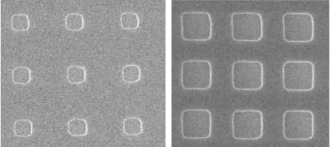
Fig. 2. Electron microscope images of 250 × 250 nm and 500
× 500 nm holes in 400 nm thick photoresist. Periods in both
directions are 1 μm.
The real part of the dielectric function is determined
in a closed form from ε2 using Kramers-Kro¨nig integra-
tion [11]. The model dielectric function employs five fit-
ting parameters: the non-dispersive term ε∞ = 1.80, the
band gap energy Eg = 1.26, the amplitude A = 5.17, the
Lorentz resonant frequency E0 = 6.53, and the broadening
parameter C = 0.11.
Reference values of CDs were taken from fit of the ellipsometric data obtained by UVISEL for spectral range
from 1 eV to 3.5 eV and typical incidence angle 70◦. The
wider spectral range of the ellipsometer provided better sensitivity to the grating depth, when compared to the polarimeter.
top CD (H) hole photoresist
top CD (H)
depth (d)
silicon
4 Optical modeling
Optical response of grating is modeled by a 2D version
of standard rigorous coupled-waves method (RCWM) [12]
based on a pro jection of Maxwell equations to a Fourier basis and reducing them to a set of ordinary differential equations.
Implementation is extended by using factorization of
permittivity tensor based on the Li inverse rules [13] and
boundary conditions on each interface are treated by
scat-Fig. 3. Schematic picture of the grating profile. Critical di-
mension of the grating is hole width denoted by H . Depth of the hole in resist layer is denoted by d.
azimuth, the former from 45◦ to 70◦ (limited by the spot
size) and the latter over all possible values from 0◦ to 360◦.
tering matrix (S-matrix) algorithm [14]. RCWA with these
two extensions is nowadays standard approach to the 1D lamellar and 2D dot gratings. It leads to very fast calcu- lations, where only relatively small number of the Fourier harmonics is necessary and also avoids numerical insta- bility otherwise appearing in the cases of deeper gratings. Further, eigenvalue problem was tweaked the way, that
In this work, the azimuth was varied from −90◦ to 90◦ in
steps of 5◦. only about 50−
their signific 75% of modes were used depending onThis alone allowed to further decrease
3 Sample characteristics
Samples of 2D periodic gratings were prepared in CEA – LETI by using UV lithography process. These gratings consisted of square arrays of square holes in 400 nm thick layers of photoresist deposited on crystalline silicon. Grat-ing period was 1 μm in both directions, while nominal dimensions of holes were 250 × 250 and 500 × 500 nm. Critical dimension (CD) to be determined by fitting the data are hole width and depth. Electron microscopy
im-ance.
calculation time by about a factor of two, while the preci-sion of the calculations did not exhibit significant changes. The code provides the complex Jones matrix of zero diffraction order of the grating
J = J11 J12
l
. (5)
J21 J22
The corresponding Mueller matrix M can be calculated from the Jones matrix J and expressed in the form of four block matrices:
⎡ M
11 M12 M13 M14 ⎤
ages and schematic picture of the sample are shown in
Figures 2 and 3.
Optical function of photoresist was determined from ellipsometric measurement on a non-patterned part of the
M = ⎢ M21 M22 M23 M24 ⎢ ⎣ M31 M32 M33 M34 ⎦ M41 M42 M43 M44 B11 B12 B21 B22 l , (6)
sample and material parameters of crystalline silicon were
taken from Palik [10]. Photoresist is transparent in lower
where the expressions for the block matrices follows:
I 2 I 2 − J 2 2 l
energy spectrum, but exhibits absorption in the ultra- B11 = 2 2 2 2 12 2 − J222 , (7)
violet part of the spectrum. In the selected spectral range I − J21 − J22 I − J12 − J21
1 − 3.5 eV optical function of photoresist was modeled by B
12 =
(P
1112+ P2122) −8<(P1112+ P2122) l, (8)
the Tauc-Lorentz model [11], which imaginary part of the
complex dielectric function is given by:
B21 = (P1112 − P2122 ) −8<(P1112 − P2122 ) (P 1121 + P1222 ) (P1121 − P1222 ) l , (9) ⎧ 1 AE C(E − E )2 8<(P1121 + P1222 ) 8<(P1121 − P1222 ) ⎨ 0 g (E > E g ) ε2(E) = ⎩E (E2 − E2)2 + C2 E2 0 (E ≤ Eg ) . (4) B22 = (P 1122 + P1221 ) −8<(P1122 − P1221 ) l 8<(P1122 + P1221 ) (P1122 − P1221 ) . (10)
354 The European Physical Journal Applied Physics V ) Here J 2 denotes |J ij |2, I 2 = 1 (J 2 + J 2 + J 2 + J 2 ), and ij Pijkl = J ∗ kl 2 11 12 21 22 ij J
. As the absolute reflectivity of the system is unknown, sample is characterized by a normalized Mueller
matrix Mn, which is related to M by the simple relation
Mn = I − 2M.
Block matrix B11 from (7) contains information about
reflectivities, where in our case of normalized Mueller ma-trices the total reflectivity of the system is unknown. Block
B22 in (10) is connected to the ellipsometric parameters,
where for isotropic samples the following relations hold:
Is = M43 = −M34, Ic = M33 = M44. Ellipsometric pa-
rameters Is and Ic can be written by using ellipsometric
angles ψ and Δ as in (1) and (2), respectively. Off-diagonal
blocks B12 and B21 from (8) and (9) are adherent to an
anisotropic behavior of gratings. In our case B12 and B21
are zeros when grating is in planar configuration or
ro-tated by azimuthal angle of 45◦ (due to the symmetry of
square profiles of holes). Note that our gratings are sym-
metrical to the azimuthal angle rotation by 90◦, therefore
two equal planar configurations exist.
(a) 250 nm holes (b) 500 nm holes
Fig. 4. (Color online) Error estimation ΔH of CD, plotted for
range of incidence θ and azimuthal angles φ. Errors are noted by different colours with values found in the bar on the right, values are in nanometers. Figure is obtained from simulated data calculated every 5◦ of incidence and azimuthal angle.
The variance-covariance matrix of the parameters is then
given by [15]:
5 Fitting and optimal measurement
configuration
Sensitivity of fitted parameters to the experimental data and correlations between them can be studied by using
V = σ2 (JT J)− 1· (13)
The diagonal elements Vii correspond to the squares of
standard deviations of parameters. The correlations Cij
between different parameters can be obtained from the off-diagonal elements of V (the parameter covariances) as:
Vij
rigorous modeled data with applied white noise of ampli-
tude √3σ, where σ is estimated precision of experimental
Cij =
iiVjj
· (14)
data. In our work σ is chosen equal to 0.01, which is close to the experimental precision of our measurement setup.
Used fitting parameters of the model are only two – critical dimension (H ) and grating depth (d). Merit func- tion relating our model to experimental data used in this section is defined as
In principle, these formulas are valid only in the ideal case of purely statistical additive noise, not necessarily Gaussian but with a uniform and finite RMS value σ. Moreover, the noises affecting different experimental data are supposed to be fully decorrelated. Even though these assumptions are not fulfilled in our case (as in most real situations) this procedure is the only one which can be
rea-K M meas M calc (H, d 2 sonably implemented to optimize the measurement config-f merit (H, d) = 1 ) ) ijk − 2ijk , urations and it provides useful results, as shown below.
15K − 3 k=1 i,j σijk
(11)
The variance-covariance matrices and corresponding
correlation matrices are evaluated for the range 0−70◦ of
where k denotes the spectral point from the total number
K , indexes i, j denote all Mueller matrix elements except
M11 and experimental errors σijk are taken all equal to σ = 0.01. This assumption of uniform noise over all values
of indexes i, j, k would be rigorously justified only for ideal situations, with a perfectly adequate model and a purely statistical noise with no systematic errors. As discussed below, in reality this is not the case, but this assumption is adequate enough to derive the optimal configurations from “virtual experiments” based only on simulations and on the standard evaluation of the parameter variances and correlations outlined below.
Considering a set of experimental data Mr (in our case
these would be the Mijk Mueller matrix elements, with the
three indexes i, j and k lumped into a single index r) and
a set of parameters βs (in our case H and d) we define the
(rectangular) Jacobian matrix J by
∂Mr
incidence angles θ and 0−90◦ of azimuthal angles φ with
the step of 5◦ in both. The modelled experimental data are
normalized Mueller matrices in the 450–825 nm spectral range.
The standard errors of H corresponding to 95%
con-fidence interval are plotted in Figure 4 for both grating
samples. From the figure one can immediately conclude that the grating with 500 nm holes has much better de-termined values of H and d for all possible configurations. The reason for this is the big difference between fill factors of the two gratings (1/4 and 1/16), together with the fact that 250 nm holes are smaller than all the wavelengths of incident light. Nevertheless, the trends are the same in both figures, showing decreasing errors with increasing angles of incidence. Higher values of errors for azimuthal
angles around 45◦ and incidence angles around 70◦ suggest
that experimental configurations close to planar configu- ration should be preferred.
The errors in determination of grating depth d are
Jrs = ∂β
s
ter, in some cases under 0.2. This is nice example of the fact that higher incidence angle is not always better and it also shows usefulness of presented approach to choose advantageous experimental configuration.
6 Results and discussions
(a) 250 nm holes (b) 500 nm holes
Fig. 5. (Color online) Error estimation Δd of the grating
depth, plotted for range of incidence and azimuthal angles. Statistical errors are expressed in nanometers.
(a) 250 nm holes (b) 500 nm holes
Fig. 6. (Color online) Correlation coefficient between fitted
parameters H and d plotted for range of incidence and az- imuthal angles. Values for different colours can be found in the bar on the right. Figure is plotted from data calculated every 5◦ of incidence and azimuthal angle.
precisely determined except incidence angles close to nor- mal incidence. Therefore, preferences are the same as in the case of ΔH towards the higher angles of incidence.
A very interesting situation can be observed at Fig-
ure 6, where correlation coefficient between H and d is
plotted. The plot for 250 nm holes shows smaller corre- lations between parameters for smaller incidence angles. Though, when one shall decide for more advantageous con- figuration, errors in the parameters are more important. Smaller correlation would lead to a smoother fitting, but the precision of the fitted result would not be that good. Therefore, we look for the configurations with relatively small errors with not so bad correlations. In the case of the sample with 250 nm holes an advantageous
configu-ration is at incidence angle as big as 70◦ and azimuthal
angle close to 0◦ (planar configuration). At that
configu-ration the errors of fitted parameters are the smallest and correlation coefficient is under 0.8.
Sample with 500 nm holes features a surprising re- sult. On one hand, one can naturally think of the same configuration as for the case with 250 nm holes with
inci-dence angle of 70◦ and azimuthal angle close to 0◦.
Sur-prisingly though, the better choice is incidence angle of
45◦ for almost any choice of azimuthal angle. Errors in
fitted parameters are about the same as for high incidence angles, while correlation between parameters is much
bet-Based on the results reported above, polarimetric mea- surements of the 250 × 250 nm sample were accomplished
by MM16 for incidence angle of 70◦, while azimuthal
an-gles was varied from −90◦ to 90◦ in steps of 5◦.
Polarime-ter provides normalized Mueller matrices for the spectral range of wavelengths from 450 to 825 nm. The sample with 500 × 500 nm holes was measured with the same az-
imuths, but with incidences varying from 45◦ to 70◦ in
steps of 5◦. In this work we fitted the data by using
non-linear Levenberg-Marquardt method [15], which typically
converges very fast to minimum if suitable initial condi- tions are chosen.
The results of the fits of Is and Ic data measured for
both samples in planar configuration at incidence angle of
70◦ are plotted in Figure 7. Measured data are denoted
by squares and rounds in the figure. Curves of measured data for the 250 nm holes sample are very smooth and simple and the quality of the fit is better than for 500 nm holes. During fitting only 50 points were used as inclusion of more points increases significantly computation time and does not provide much more information. Fitted pa-rameters of two samples give the values of CDs 250.3 and 497.4 nm and depths 393.5 and 406.1 nm, which will be compared with the results of the fits of polarimetric data. To compare the ellipsometric fit with polarimetric ones on the sample with 250 nm holes, data for all azimuthal angles (each one separately) with 30 spectral points were
fitted and results are plotted in Figure 8. Spectral points
are chosen equidistantly from the wavelength range of
450–850 nm shown in Figure 9. Zero azimuthal angle is
set to the planar configuration, with the incidence plane
parallel to hole walls. Incidence angle is 70◦ in all cases.
Comparison with the values from ellipsometric fit gives very good correspondence between both values – CD and grating depth.
Parameters are quite uniform over the whole range of 37 azimuthal angles, which leads to the conclusion that model describes very well the measured data. To be more quantitative, we estimated the errors of these pa-
rameters (with 95% confidence intervals) by equation (13)
with σ equal to the experimental RMS deviation between data and fits. The estimated error of the CD (H ) was 1.93 nm, which is much larger than the fluctuations of this parameter with azimuthal angle: this unexpected con-stancy may come from the influence of the initial guess (which was kept constant at 250 nm) on the final result of the Levenberg-Marquardt algorithm. Conversely, for the thickness d the estimated error was 0.15 nm, which is much smaller than the observed variations of d with the azimuth, a more common behavior which can be due to small systematic errors and/or model inadequacies.
356 The European Physical Journal Applied Physics
D e pt h [n m] T o p CD [ n m ] 1 0.5 0 −0.5 250x250 nm holes I data s I data c I fit s I fit c 252 251 250 249 −1 395 1 0.5 0 −0.5 −1 500x500 nm holes I data s I data c I fit s I fit c 394 393 392 −90 −80 −70 −60 −50 −40 −30 −20 −10 0 10 20 30 40 50 60 70 80 90 Azimuthal angle [deg]
Fig. 8. (Color online) Results of fits of of 250 nm holes in
1 1.5 2 2.5 3 3.5 Photon energy [eV]
Fig. 7. (Color online) Fits of the ellipsometric parameters Is
resist. Incidence angle was 70◦ . Data for each azimuthal angle (with step of 5◦ ) were fitted independently. Top part of figure shows fitted values of top CD, while bottom part the grating depth. Units are in nanometers.
and Ic of 250 nm (top) and 500 nm (bottom) holes in resist. Incidence angles were 70◦ in both cases. Fitted values of CDs are 250.3 and 497.4 nm and depths are 393.5 and 406.1 nm, respectively.
Typical values of the off-diagonal elements B12 and B21
of the Mueller matrix are very small, which means that this grating embodies only slight anisotropic behavior if it is rotated. This is obviously due to the high symmetry of the sample and small volume fill factor of holes (1/16). Moreover, data are basically sensitive only to fill factor of the holes and it seems impossible to distinguish any other details about profile (e.g. round corners). Example
of typical data and the fit can be found in Figure 9 for
azimuthal angle 30◦. Fit corresponds very well to data in
all elements of normalized Mueller matrix, including off-diagonal ones with small values.
The results of Section 5 shows that data taken with
1.05 1 0.95 1 0 −1 0.05 0 −0.05 0.05 0 −0.05 450 550 650 750 850 1 0 −1 1.05 1 0.95 0.05 0 −0.05 0.05 0 −0.05 450 550 650 750 850 0.05 0 −0.05 0.05 0 −0.05 1 0 −1 1 0 −1 450 550 650 750 850 0.05 0 −0.05 0.05 0 −0.05 1 0 −1 1 0 −1 450 550 650 750 850
the 500 nm holes sample is much richer, which motivated us to measure the sample at six different incidence angles:
45−70◦. The results of fitting procedures can be seen on
Figure 10, where the non-uniformity of fitted parameters
can be observed. Note that every point in the plot corre-sponds to a measurement followed by a fit.
Regarding rectangular profile of the holes, there is nec-essary symmetry with respect to the zero angle and also
−90◦ and 90◦. Also, if profile is perfectly square, there
are other symmetries with respect to the azimuthal an-
gles −45◦ and 45◦. Typical data and the fit can be found
in Figure 11 at incidence angle of 45◦ and azimuthal angle
30◦.
The average estimated errors in the CD and the grat-
ing depth for the 500 nm holes grating at 45◦ incidence
are 1.14 nm and 0.28 nm within 95% confidence interval. In contrast with the 250 nm holes sample, these values are well below the observed variation of both H and d
with the azimuth. Figure 10 shows this variation for all
Fig. 9. (Color online) Example of the data (blue points) and
fit (red lines) of the normalized Mueller matrices of the sam-ple with 250 nm holes. Wavelengths are marked on x-axis, az- imuthal angle in this case was 30◦ and angle of incidence 70◦ .
investigated incidence angles. The fits at the smallest in-
cidence angle of 45◦ are the most uniform. From Figure 6
we know that the standard errors and correlation between
parameters at 45◦ are better than for the other angles. On
the other hand, higher incidences feature decreased sensi- tivity and increased parameter correlations. Therefore, we assume that not only experimental errors are responsible for the non-uniformity of the fitted values, but also worse conditions of fits at higher incidence angles.
The residual differences between measured data and
fit are plotted in Figure 12 for the 500 nm holes
grat-ing measured at 45◦ incidence in the planar
D ept h [n m ] T o p CD [n m ] 520 510 500 490 0.03 0.015 45 0 50 −0.015 55 −0.03 60 65 0.1 70 0.05 0 −0.05 −0.1 0.1 0.05 0 −0.05 −0.1 0.03 0.015 0 −0.015 −0.03 0.03 0.015 0 −0.015 −0.03 0.03 0.015 0 −0.015 −0.03 0.03 0.015 0 −0.015 −0.03 0.03 0.015 0 −0.015 −0.03 410 408 406 404 402 400 −90 −75 −60 −45 −30 −15 0 15 30 45 60 75 90 Azimuthal angle [deg]
0.03 0.015 0 45 −0.015 50 −0.03 55 60 0.03 65 0.015 70 0 −0.015 −0.03 450 650 850 0.03 0.015 0 −0.015 −0.03 0.03 0.015 0 −0.015 −0.03 450 650 850 0.1 0.05 0 −0.05 −0.1 0.1 0.05 0 −0.05 −0.1 450 650 850 0.1 0.05 0 −0.05 −0.1 0.1 0.05 0 −0.05 −0.1 450 650 850
Fig. 10. (Color online) Fitted values of top CD and grating
depth of the sample with 500 nm holes in nanometer scale. Curve correspond to the incidence angles marked on the right side of figure. Each point corresponds to one measurement and fit.
Fig. 12. (Color online) Residual difference between measured
data and fit for 500 nm holes grating at 45◦ incidence and 0◦ azimuth. In this configuration the theoretical off-diagonal elements vanish.
measured data exhibit clear symmetry properties with
re-1.05 1 0.95 1 0 −1 0.4 0.2 0 −0.2 0.4 0.2 0 −0.2 1 0 −1 1 0.9 0.8 0.4 0.2 0 −0.2 0.4 0.2 0 −0.2 0.4 0.2 0 −0.2 0 −0.1 −0.2 1 0 −1 1 0 −1 0.4 0.2 0 −0.2 0.4 0.2 0 1 0 −1 1 0 −1
spect to matrix transposition. These symmetries are ob- viously not compatible with the statistically independent
noise properties assumed in Section 5, and are probably
due to model inadequacies rather than measurement sys- tematic errors, as such errors are not expected to preserve transposition symmetries with the calibration method used for the MM16. In any case, a rigorous treatment of such inadequacies is not available (one has only to change the model, if possible). However, the standard treatment
implemented in Section 5 seems a quite reasonable first
step to optimise the measurement configuration.
To compare virtual and real experiments, the correla- tions obtained from regression of measured data and “vir-
tual experiments” were plotted in Figure 13b. Top part of
the plot corresponds to the virtual experiment and bottom to the regression results. Very good correspondence is ob- served for all of the measured configurations. The values
450 550 650 750 850 450 550 650 750 850 450 550 650 750 850 450 550 650 750 850
of the statistical errors are in the same manner compared
Fig. 11. (Color online) Example of the data (blue points)
and fit (red lines) of the normalized Mueller matrices of the sample with 500 nm holes. Azimuthal angle is 30◦ and angle of incidence is 45◦ .
normalized Mueller matrices are expected to vanish in this configuration, we can say that non-zero signals in off- diagonal elements are due to experimental errors, such as noise and systematic errors including azimuthal position- ing. Full Mueller matrix measurements do provide some useful criteria to unveil such errors: for example the peaks observed in most elements around wavelengths of 675 nm involve a small depolarization of the emerging light, which is certainly due to measurement inaccuracies in this spec- tral region where the reflectivity drops to its lowest val- ues, of the order of 2% and less. Moreover, we see on this figure that the residual differences between model and
in Figure 13c for hole width and Figure 13d for grating
depth. The higher values from measurement regressions can be explained by the map of merit function plotted
in Figure 13a, where for some angles the values are more
than five times bigger than in virtual experiments. The observed values of the regression statistical errors in Fig-
ures 13c and 13d are smaller than parameter dispersion
in Figure 10, while inconsistent values appeared for the
azimuthal angles with higher values of merit function in
Figure 13a. At this moment, we can conclude that ideal
model of experiment can be only a starting point to the determination of the optimal configuration, but it can- not fully replace actual measurement, which in general involves some systematic errors.
To increase sensitivity of parameters to the measured data, each azimuthal was fitted separately, but this time for all the incidence angles together. As this is very
358 The European Physical Journal Applied Physics D ept h [ nm ] T op C D [ nm ]
Fig. 13. (Color online) Results of regression analysis of data
520 515 510 505 500 495 490 −90 −80 −70 −60 −50 −40 −30 −20 −10 0 10 20 30 40 50 60 70 80 90 Azimuthal angle [deg]
410 408 406 404 402 −90 −80 −70 −60 −50 −40 −30 −20 −10 0 10 20 30 40 50 60 70 80 90 Azimuthal angle [deg]
Fig. 14. (Color online) Fitted values of top CD and grating
depth for the 500 nm holes sample. Data for incidence angles from 45◦ to 70◦ with step of 5◦ were fitted simultaneously for each azimuthal angle.
measured on the sample with 500 nm holes. (a) Values of the merit function for the optimal values of parameters. (b), (c) and (d) Comparison of statistical uncertainties and correlations of the H and d parameters deduced from virtual (top plots) and actual experiments (bottom plots). Values are plotted for all measured incidence angles from 45◦ to 70◦ (y-axis) and range 0–90◦ of azimuthal angles (x-axis).
time consuming procedure, only eight points with wave- lengths from the range between 475 and 825 nm were cho- sen. To decrease calculation time, initial values for every azimuthal angle were taken from fitted values at previ- ous angle, except the first one. This does not have high influence on the results – it was compared with fits from
1.05 1 0.95 1 0 −1 0.5 0 −0.5 0.5 0 −0.5 1 0 −1 1 0.9 0.8 0.5 0 −0.5 0.5 0 −0.5 0.5 0 −0.5 0.5 0 −0.5 1 0 −1 1 0 −1 0.5 0 −0.5 0.5 0 45 −0.5 50 55 1 60 65 70 0 −1 1 0 −1
the constant initial values and no significant differences were observed. On the other hand, fitting started rela- tively close to minimum and total time was decreased by excluding some unnecessary iterations in the beginning.
Results of the fits in Figure 14 show much more uni-
form distribution of fitted values, which was expected from mixing multiple incidence angles data together. Errors in the CD and the grating depth are in the average 0.54 nm and 0.22 nm within the confidence interval of 95%, which gives better confidence of the CD values than in the sepa- rate fits. The remaining non-uniformity of the fitted values is probably caused by experimental errors and also simpli- fication of the model, which assumed square profile of the
holes. From the electron microscope images in Figure 2
one can notice rounding corners of the holes. Some imper-
fections of the fits can be seen in Figure 15, which also
indicates that the model does not perfectly correspond to the data. More complex profiles were not used in this work as this would have significantly increased calculation time, while at the end, simpler model provided sufficient accuracy. For the same reasons only eight spectral points
450 550 650 750 850 450 550 650 750 850 450 550 650 750 850 450 550 650 750 850
Fig. 15. (Color online) Example of the data (points) and fit
(lines) of the normalized Mueller matrices of the sample with 500 nm holes at azimuthal angle 30◦ . Data for the incidence angles 45–70◦ marked on the right side of plot were fitted to-gether.
were used during fitting to decrease calculation times to a manageable amount.
7 Conclusions
Two samples with square arrays of square holes in a pho- toresist layer on silicon were characterized by spectral ellipsometry and Mueller matrix polarimetry. Both tech- niques gave close values of critical dimensions. Data from UVISEL provided more precise data in planar geometry due to wider spectral range, while MM16 shows higher robustness by enabling user to choose any experimental configuration.
We showed that the sample with smaller holes exhibits very small in-plane anisotropy, which permits to determine only critical dimensions without any further information about profile. On contrary, sample with bigger holes shows slight non-uniformity of the critical dimensions, which gives a clear indication that more details about the profile can be in principle extracted from the data.
Comparison of the confidence intervals of fitted param-eters has shown correspondence between theoretical “vir-tual experiments” and the measurements on the Mueller matrix polarimeter. This result shows that theoretical cal-culations can be used to estimate optimal measurement configuration in the cases where the overall measurement precision is at least approximately known.
We have demonstrated that theoretical study to esti-mate optimal measurement configuration is very useful, sometimes even unavoidable, to get precise and reliable results from a single measurement. Statistical quantities including parameter errors and correlation coefficient were compared between “virtual experiment” and measurement regression, showing excellent agreement between parame-ter correlations. Dispersion of the optimal values for dif-ferent azimuthal angles is higher than statistical errors obtained from regressions, which means that systematic errors and and/or model inadequacies played crucial role in the final precision of the regression. Therefore, the typ-ical sensitivity calculations based on virtual experiments and a model a priori assumed to be ideal provide a good starting point to the determination of the optimal config-uration, but it cannot fully replace actual measurement.
References
1. B.J. Rice, H. Cao, M. Grumski, J. Roberts, Microelectr. Eng. 83, 1023 (2006)
2. T. Novikova, A. De Martino, P. Bulkin, Q. Nguyen, B. Dr´evillon, V. Popov, A. Chumakov, Opt. Expr. 15, 2033 (2007)
3. H.T. Huang, F.L. Terry Jr., Thin Solid Films 468, 339 (2004)
4. H.T. Huang, W. Kong, F.L. Terry Jr., Appl. Phys. Lett.
78, 3983 (2001)
5. T. Novikova, A. De Martino, S.B. Hatit, B. Dr´evillon, Appl. Opt. 45, 3688 (2006)
6. R.M.A. Azzam, N.M. Bashara, Ellipsometry and Polarized
Light, 2nd edn. (North-Holland, Amsterdam, 1987)
7. E. Compain, S. Poirier, B. Dr´evillon, Appl. Opt. 38, 3490 (1999)
8. J. Tyo, Opt. Lett. 25, 1198 (2000)
9. E. Garcia-Caurel, A. De Martino, B. Dr´evillon, Thin Solid Films 455-456, 120 (2004)
10. Handbook of Optical Constants of Solids I and II and III, edited by E.D. Palik (Academic Press, 1991)
11. G.E. Jellison Jr., F.A. Modine, Appl. Phys. Lett. 69, 371 (1996)
12. M.G. Moharam, T.K. Gaylord, J. Opt. Soc. Am. 72, 1385 (1982)
13. L. Li, J. Opt. Soc. Am. A 13, 1870 (1996) 14. L. Li, J. Opt. Soc. Am. A 13, 1024 (1996)
15. W.H. Press, S.A. Teukolsky, W.T. Vetterling, B.P. Flannery, Numerical Recipes in C++. The art of
scien-tifique computing, 2nd edn. (Cambridge, 2002)
To access this journal online: www.edpsciences.org