Conditioning, reduction, and disturbance analysis of large order integrated models for space-based telescopes

Conditioning, Reduction, and Disturbance Analysis of

Large Order Integrated Models for Space-Based Telescopes

by

Scott Alan Uebelhart

S.B. Aeronautics and Astronautics

Massachusetts Institute of Technology, 1998

Submitted to the Department of Aeronautics and Astronautics

in partial fulfillment of the requirements for the degree of

Master of Science in Aeronautics and Astronautics

at the

MASSACHUSETTS INSTITUTE OF TECHNOLOGY

February 2001

@

Massachusetts Institute of Technology 2001. All rights reserved.

A uthor ... ...

Department of Aeronautics and Astronautics

February 1, 2001

Certified by ...

...

...

David W. Miller

Associate Professor

Thesis Supervisor

A ccepted by ...

Wallace E. Vander Velde

Professor of Aeronautics and Astronautics

Chair, Committee on Graduate Students

MASSACHUSETTS INSTITUTE OF TECHNOLOGY

Conditioning, Reduction, and Disturbance Analysis of

Large Order Integrated Models for Space-Based Telescopes

by

Scott Alan Uebelhart

Submitted to the Department of Aeronautics and Astronautics on February 1, 2001, in partial fulfillment of the

requirements for the degree of

Master of Science in Aeronautics and Astronautics

Abstract

A new fleet of flexible space observatories is being prepared to follow up on the success of the Hubble Space Telescope. The Next Generation Space Telescope (NGST) and the Space Interferometry Mission (SIM) are being designed at NASA centers for launch within the decade. In addition, the on-orbit testbed Nexus was planned as a precursor mission to NGST. Because of their stringent optical requirements, detailed integrated models of these spacecraft are being assembled to simulate their performance in the presence of disturbance forces and optical control loops. The Dynamics, Optics, Controls, and Structures (DOCS) toolbox is used to model and assemble the individual components of the integrated system, and to run dynamical analyses of the spacecraft for the purpose of design iterations.

These integrated models, cast in state-space form, have grown beyond the small "stick" models used for initial disturbance studies, and may now have upwards of thousands of states. To lower the computational burden of the DOCS analyses, and to improve the numerical quality of the models as they are manipulated, this thesis concentrates on model quality management for large systems. This includes steps that can be taken to improve the numerical conditioning of large matrices, and methods to balance and reduce the state vectors in large systems. The linear algebra routines required for balancing are reviewed, and a faster method of solving the Lyapunov equation is introduced. A variation of the typical gramian balancing technique is used to successfully balance models that could not be balanced using traditional MATLAB tools. These models are then reduced to as little as one sixth of their original size.

A review of reaction wheel disturbances includes both broadband and discrete wheel speed models using power spectral density (PSD) curves and white noise shaping filters. Using these disturbances along with the reduced models, disturbance analyses are run that compare the open loop dynamics of NGST and Nexus, and examine the closed loop behavior of the latest and most complete SIM model. Prominent dynamical features are pointed out, and modes requiring further study are identified. A final comparison between multiple versions of the SIM model is included to judge the ability of smaller stick models to capture important spacecraft dynamics.

Thesis Supervisor: David W. Miller Title: Associate Professor

Acknowledgments

This research was supported by the NASA Goddard Space Flight Center, under con-tract NAG 5-7839 (Structural Dynamics and Controls Analysis and Simulation for NASA's

NGST), with Gary Mosier as Technical/Scientific Officer, and by JPL Contract #961123

(Modeling and Optimization of Dynamics and Control for the NASA Space Interferometry Mission and the Micro-Precision Interferometer Testbed), with Robert Grogan as Techni-cal/Scientific Officer and Dr. Sanjay Joshi as Contract Monitor.

I would like to thank Professor Dave Miller for his assistance and support, and for his perseverance in showing me the path for this thesis. Many people in the Space Systems Lab deserve thanks for helping me along the way. Homero Gutierrez, Greg Mallory, and Jeremy Yung all provided their time and insights to help me understand linear systems theory. I wish to particularly thank Oli de Weck for providing guidance and suggestions, and for proof-reading this entire document. Gary Mosier at NASA Goddard provided a desk for the summer and the opportunity to let me watch the actual spacecraft design process.

Becky Masterson provided waterfall plots, generous amounts of MATLAB and LATEX advice, and a guest room by the beach. Alice Liu was a kind listener who was there for all of my controls questions. Special thanks go to Laila Elias, who walked side-by-side with me through writing a thesis and earning a pilot's license. Alvar Saenz Otero was there with a patient ear and candy.

SharonLeah Brown and Peggy Edwards both keep the lab running smoothly. Marie Stuppard has provided immeasurable amounts of assistance ever since I arrived at MIT many years ago, and continues to have the warmest smile in the department.

A thanks goes to all of my friends who would talk about things other than research, including my office mates Seung Chung and Elisabeth Lamassoure, my housemate Shawn Kelly, Patrick Trapa and Tim Glenn, Alissa Clawson, and especially to Nate and Zohra Rawling, for putting up with me for so long.

And the final and warmest thanks to Granny, Lori, and Mom and Dad, for helping me get to this point in the first place, and for supporting me, together as a family.

Contents

1 Introduction

1.1 M otivation . . . .

1.2 Dynamics, Optics, Controls, Structures (DOCS)

Framework . . . .

1.3 State Space Balancing and Reduction Routines .

1.4 Thesis Overview . . . .

2 Space Telescope Descriptions

2.1 Next Generation Space Telescope (NGST) . . . .

2.1.1 NGST Mission Architecture . . . .

2.1.2 NGST Structural Finite Element Model .

2.1.3 NGST Optical Performance . . . .

2.2 N exus . . . .

2.2.1 Nexus Mission Architecture . . . .

2.2.2 Nexus Structural Finite Element Model .

2.2.3 Nexus Optical Performance Metrics . . .

2.3 Space Interferometry Mission (SIM) . . . .

2.3.1 SIM Mission Architecture . . . .

2.3.2 SIM State-Space Model . . . .

2.4 Sum m ary . . . .

3 Numerical Tools

3.1 Eigenvalues . . . .

3.2 Singular Value Decomposition . . .

3.2.1 Properties of SVD matrices 21 21 23 24 26 29 . . . . 30 . . . . 32 . . . . 33 . . . . 35 . . . . 36 . . . . 37 . . . . 38 . . . . 40 . . . . 41 . . . . 42 . . . . 45 . . . . 49 51 52 53 54

3.2.2 Condition Number of Matrices . . . . 56

3.3 Lyapunov Equation . . . . 58

3.3.1 Controllability and Observability Gramians . . . . 58

3.3.2 Analytical Solution . . . . 60

3.3.3 Fast Lyapunov Solvers . . . . 61

3.4 Summary . . . . 67

4 Methods for Maintaining Model Quality 69 4.1 Model Preparation . . . . 69

4.1.1 Rigid Body Modes . . . . 71

4.1.2 Low- and High- Frequency Modes . . . . 72

4.1.3 Input/Output Selection . . . . 73

4.2 Tracking Numerical Quality . . . . 76

4.3 Summary . . . . 78

5 Balancing and Model Reduction 81 5.1 Methods of Model Reduction . . . . 81

5.2 Balancing Routines . . . . 83

5.2.1 Gramian Transformations . . . . 84

5.2.2 Eigenvalue Approach . . . . 87

5.2.3 SVD Approach . . . . 87

5.3 Balancing Routines on Large Models . . . . 89

5.3.1 Difficulties . . . . 89

5.3.2 Balanced Truncation Method . . . . 91

5.4 Reducing the Model . . . . 94

5.5 Spacecraft Examples . . . . 100

5.5.1 NGST . . . . 100

5.5.2 SIM . . . . 105

5.6 Summary . . . . 116

6 Disturbance Sources 119 6.1 Reaction W heel Disturbances . . . . 119

6.3 Broadband Wheel Speed Model . . . .

6.4 Discrete Wheel Speed Model . . . .

6.5 Summary . . . .

7 Disturbance Analysis

7.1 Integrated Modeling . . . .

7.1.1 Structural, Optical, and Disturbance models 7.1.2 ACS and Optical Controllers . . . .

7.2 Disturbance Analysis Methodology . . . .

7.3 PSD Analysis on Nexus & NGST . . . .

7.3.1 Broadband wheel speeds . . . . 7.3.2 Discrete wheel speeds . . . .

7.3.3 Nexus/NGST Analysis Summary . . . .

7.4 Lyapunov and PSD Analysis on SIM . . . .

7.4.1 Lyapunov Analysis . . . .

7.4.2 Reaction Wheel Comparison . . . .

7.4.3 Frequency-based PSD Analysis . . . .

7.4.4 State-Space versus Tonal Comparison . . . .

7.4.5 SIM Analysis Summary . . . .

7.5 Sum m ary . . . . . . . . 136 . . . . 137 . . . . 140 . . . . 143 . . . . 143 . . . . 148 . . . . 151 . . . . 151 . . . . 152 . . . . 156 . . . . 159 . . . . 165 . . . . 167 . . . . 168 8 Model Evolution

8.1 SIM Classic Version 1.0 . . . .

8.2 M odel Com parison . . . .

8.3 Sum m ary . . . .

9 Conclusions

9.1 O verview . . . .

9.2 Recommendations for Future Work . . . .

A Nexus/NGST Disturbance Analysis Results Comparison

B SIM Lyapunov Disturbance Analysis Results C SIM PSD Disturbance Analysis Results

126 128 133 135 135 169 170 171 176 177 177 181 185 195 201

List of Figures

1-1 Overview of the DOCS framework. . . . . 24

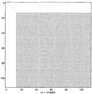
1-2 Structure of the SIM state-space A matrices . . . . 25

1-3 Thesis O utline . . . . 28

2-1 Earth-Sun Lagrangian points. . . . . 30

2-2 NGST designs proposed by the contractor candidates and GSFC [5] . . . . 31

2-3 ngst603ss FE Model . . . . 34

2-4 Original Nexus/Horizon spacecraft . . . . 37

2-5 Current Nexus design . . . . 38

2-6 Nexus stowed configuration in a Delta II fairing. . . . . 39

2-7 Nexus/Horizon Finite Element Model . . . . 40

2-8 Primary Mirror of the Reduced Nexus/Horizon FEM . . . . 41

2-9 Comparison of modal frequencies between high- and low-fidelity Nexus/Horizon m odels . . . . 42

2-10 An artist's drawing of the Space Interferometry Mission [6] . . . . 43

2-11 Basic elements of the SIM interferometer . . . . 44

2-12 SIM Finite Element Model . . . . 45

2-13 Devices used in SIM's optical train . . . . 46

3-1 Complex conjugate poles on the complex plane . . . . 52

3-2 CPU Time in minutes to solve a Lyapunov equation of size n using blocks of size m . . . . 64

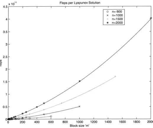
3-3 Number of flops for the sample problem, along with curves showing the flop count approximation . . . . 66

4-2 Structure of the system A matrix after appending RBMs. . . . . 72

4-3 Distribution of modal frequencies in SIM Version 2.0 . . . . 73

4-4 Sample transfer functions show the effect of units on the relative importance

of modes. ... ... 74

4-5 SIM Version 2.0 controllability gramian singular values, comparing reaction

wheel inputs alone to reaction wheel and PZT and voice coil actuators. . . 76

4-6 Transfer function of RWA F, to Star OPD #1 for SIM model v2.2 . . . . . 77

4-7 Singular values of SIM model v2.2 A matrices. . . . . 79

5-1 Hankel Singular Values for ngst603ss 200-state model . . . . 90

5-2 RWA force X to centroid X transfer function for ngst603ss 200-state model 90

5-3 Outline of the balanced truncation routine. . . . . 92

5-4 Structure of A matrices through balancing . . . . 94

5-5 Modal Frequencies of the ngst603ss 600-state and reduced 100-state models. 100

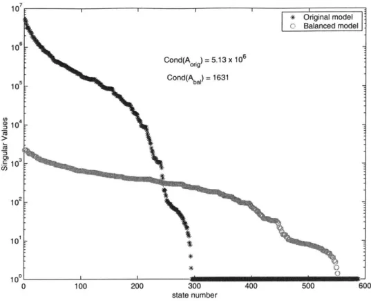
5-6 Singular Values of the NGST gramians . . . . 102

5-7 Original and balanced A-matrix singular values for ngst603ss. . . . . 103

5-8 Full order versus Balanced Transfer Function: RWA F, to Centroid X . . . 103

5-9 Transfer Function between RWA force X and centroid X, NGST 100-state

reduced m odel. . . . . 106

5-10 Transfer Function between RWA torque X and centroid X, NGST 100-state

reduced m odel. . . . . 106

5-11 Transfer Function between RWA force Y and centroid Y, NGST 100-state

reduced m odel. . . . . 107

5-12 Transfer Function between RWA force Y and the first ray's WFE, NGST

100-state reduced model . . . . . 107

5-13 A comparison of reduction methods: brutal truncation versus static

conden-sation... ... 108

5-14 Comparison of original and reduced frequencies for SIM v2.0. . . . . 109

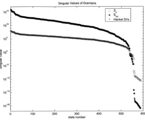
5-15 Controllability and augmented observability singular values and Hankel Sin-gular Values for SIM v2.0 . . . . 110 5-16 Singular values of the system A matrices. . . . . 110

5-17 Balanced and Reduced transfer functions of RWA Force X to Star OPD #1,

SIM v2.0 . . . . 113

5-18 Balanced and Reduced transfer Functions of RWA Force X to Star X WF1 Tilt #1, SIM v2.0 . . . . 114

5-19 Balanced and Reduced transfer Functions of RWA Torque X to Internal Metrology Opd #1, SIM v2.0 . . . . 115

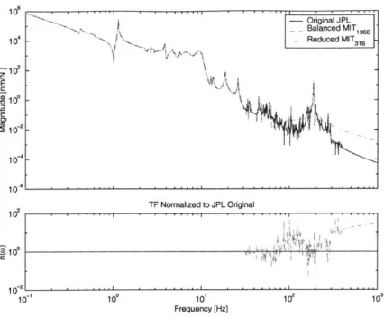
5-20 1063 state TF of RWA Force X to Star Opd #1 for SIM model v2.2 . . . . 117

5-21 608 state TF of RWA Force X to Star Opd #1 for SIM model v2.2 . . . . . 117

5-22 316 state TF of RWA Force X to Star Opd #1 for SIM model v2.2 . . . . . 118

6-1 Ithaco Type E reaction wheel [2] . . . . 120

6-2 Ithaco B-wheel waterfall plot . . . . 122

6-3 Reaction wheel frame xw, yw, z, within the spacecraft frame X,/c, Y,,, Zs/c125 6-4 Sample broadband wheel speed PSD . . . . 127

6-5 Ithaco E-wheel axial disturbance force amplitude spectra . . . . 129

6-6 Ithaco E-wheel axial disturbance force amplitude spectra: tones and state space model at 1000 RPM . . . . 132

6-7 Ithaco E-wheel axial disturbance force PSD below, and RMS above: tones and state space model at 1000 RPM . . . . 133

7-1 Effect of ACS "pseudo-controller" on Nexus/Horizon plant . . . . 138

7-2 Effect of simple ACS controller on SIM plant . . . . 139

7-3 Wave Front Error PSD and cumulative RMS plots for NGST and Nexus; broadband wheel speeds ... ... 145

7-4 Normalized Cumulative RMS WFE curves . . . . 146

7-5 Disturbance contributions to Critical WFE Frequencies . . . . 147

7-6 WFE performance PSD for Nexus/Horizon using a tonal RWA model at 1000 R P M . . . . 149

7-7 WFE performance versus wheel speed . . . . 150

7-8 Wheel harmonic numbers hi versus wheel harmonic coefficients Ci. . . . . . 153

7-9 Open and Closed Loop performance RMS versus RPM for Star OPD #1. 154

7-10 Open and Closed Loop performance RMS versus RPM for Star OPD #2. 155

7-12 Closed Loop performance RMS versus RPM for Star OPD #3 for the Ithaco

E- and B-wheels and the HST wheels. . . . . 157

7-13 Star OPD #1 open loop at 11 RPS; PSD and cumulative RMS plot. .... 161

7-14 Star OPD #1 closed loop at 36 RPS; PSD and cumulative RMS plot. . 162 7-15 Star OPD #1 closed loop at 58 RPS; PSD and cumulative RMS plot. . 163 7-16 Star OPD #1 closed loop at 66 RPS; PSD and cumulative RMS plot. . 164 7-17 Critical frequencies of Star OPD #1 at 66 RPS . . . . 166

7-18 Comparison of tonal and shaping filter PSD and RMS results for Star OPD #3 at 60 RPS. ... .. . . . ... ... . .. . . . .. .. ... . 166

8-1 SIM Version 1.0 FE model. . . . . 170

8-2 Cumulative RMS curves and PSDs for the broadband RWA disturbances . 171 8-3 Sample original and reduced transfer functions for SIM Versions 1.0 and 2.2. 172 8-4 SIM Version 1.0 cumulative RMS curve, performance PSD, and disturbance contributions for Total OPD . . . . 174

8-5 Normalized cumulative RMS curve for SIM Version 1.0, Total OPD . . . . . 175

8-6 Contributions of critical frequencies and disturbance inputs to the Total OPD RM S for SIM Version 1.0. . . . . 175

A-1 Centroid X performance PSD given a broadband wheel speed disturbance. 186 A-2 Centroid Y performance PSD given a broadband wheel speed disturbance. 187 A-3 Disturbance contribution at the critical frequencies for Centroid X. . . . . . 188

A-4 Disturbance contribution at the critical frequencies for Centroid Y. . . . . . 189

A-5 Normalized cumulative RMS performance curve for Centroid X . . . . 190

A-6 Normalized cumulative RMS performance curve for Centroid Y . . . . 191

A-7 Centroid X performance PSD given a discrete wheel speed disturbance at 1000 R P M . . . . 192

A-8 Centroid Y performance PSD given a discrete wheel speed disturbance at 1000 R PM . . . . 193

A-9 Centroid X and Y performance RMS versus Reaction Wheel Speed. . . . . 194

B-1 Star OPD open and closed loop performances . . . . 196

B-3 Star WFT open and closed loop performances. . . . . 198

B-4 FEC and External Metrology open loop performances. . . . . 199

C-1 PSD and cumulative RMS plots of Star OPD around 11 RPS . . . . 202

C-2 PSD and cumulative RMS plots of Star OPD at 19.8 RPS . . . . 203

C-3 PSD and cumulative RMS plots of Star WFT at 28.2 RPS . . . . 204

C-4 PSD and cumulative RMS plots of Star OPD and WFT at 36.0 RPS . . . . 205

C-5 PSD and cumulative RMS plots of Star OPD at 36.2 RPS . . . . 206

C-6 PSD and cumulative RMS plots of Star OPD at 58.0 RPS . . . 207

C-7 PSD and cumulative RMS plots of Star OPD at 58.6 RPS . . . 208

List of Tables

2.1 Comparison of telescopes . . . . 33

2.2 SIM v2.0 inputs for analysis . . . . 47

2.3 SIM v2.0 outputs for analysis . . . . 48

3.1 Time improvements using fast Lyapunov method . . . . 63

3.2 Improvements in flop counts using fast Lyapunov method . . . . 66

5.1 Effects of number of kept states for the NGST 600-state model . . . . 104

5.2 Effects of number of kept states on the SIM Version 2.0, 2148-state flexible model. . . . .111

6.1 Reaction Wheel Specifications [2, 14] . . . . 121

6.2 Variables to produce broadband wheel disturbance PSDs . . . . 127

7.1 Critical Frequencies in Hz . . . . 148

7.2 Summary of RMS Performances from SIM Lyapunov Analysis . . . . 158

7.3 Selection of SIM Critical RWA Speeds . . . . 160

7.4 SIM v2.2 Critical Frequencies . . . . 165

Abbreviations

ACS Attitude Control System

asec arcseconds

COBE Cosmic Background Explorer

CCA Component Cost Analysis

DOF Degree of Freedom

E03 Earth Observer 3

FE Finite Element

FEC Wave Front Tilt, Front End Camera (SIM)

FEM Finite Element Model (or Method)

FSM Fast Steering Mirrors

GEO Geosynchronous Orbit

GSFC Goddard Space Flight Center

HPF High Pass Filter

HST Hubble Space Telescope

HSV Hankel Singular Values

IMOS Integrated Modeling of Optical Systems (software package)

ISIM Integrated Science Instrument Module (NGST)

JPL Jet Propulsion Laboratory

LEO Low Earth Orbit

LOS Line-of-sight

LPF Low pass filter

MACOS Modeling and Analysis for Controlled Optical Systems (software package)

mas Milli-arcseconds

MCA Modal Cost Analysis

MSC MacNeal-Schwendler (Nastran)

MIR Mid Infrared

NGST Next Generation Space Telescope

NIR Near Infrared

ODL Optical Delay Line

OPD Optical Pathlength Difference

OTA Optical Telescope Assembly

PM Primary Mirror

PSD Power Spectral Density

PSS Precision Support Structure (SIM)

PZT Piezoelectric Translator (SIM)

RBM Rigid Body Modes

RMS Root mean square

RPM Revolutions per Minute

RPS Revolutions per Second

RSS Root Sum Squared

RWA Reaction Wheel Assembly

SIM Space Interferometry Mission

SIMTAC SIM Technical Advisory Committee

SM Secondary Mirror

SSM Spacecraft Support Module (NGST)

SVD Singular Value Decomposition

TF Transfer Function

WFE Wave Front Error

WFSC Wave Front Sensing and Control

Chapter 1

Introduction

1.1

Motivation

A decade after the launch of the Hubble Space Telescope, a new fleet of space-based obser-vatories is being prepared to look even further into the cosmos. The successors to Hubble are being designed as part of NASA's Origins Program [4], an attempt to answer the basic questions of where do we come from, and are we alone in the universe? Two of the key missions in the program are the Next Generation Space Telescope (NGST), being designed at NASA Goddard Space Flight Center, and the Space Interferometry Mission (SIM), being designed at the Jet Propulsion Laboratory. These flexible observatories will push the limits in space-based optical control. Telescope resolutions are on the order of milli-arcseconds; optical pathlengths must be controlled to within nanometers, or to within the diameters of tens of hydrogen atoms. A complete understanding of the structural dynamics of these telescopes is necessary, where even the slightest disturbance vibration could ruin science observations.

Years before any metal will be cut or mirrors polished for these instruments, their be-havior is being studied through the use of integrated computer models. All aspects of the spacecraft are examined using empirical or analytical models to simulate the expected on-orbit dynamics. Structural models are built to define the physical geometry and material properties of the spacecraft; optical models define the light paths and performance require-ments. Of particular interest are models of the disturbances; the identification of potential disturbance sources, whether from on-board reaction wheels, cryocoolers, fuel sloshing, or from external solar pressures or gravity gradients, is followed by the modeling of these

ex-citations to simulate their effects on-orbit. The basic integrated models may also contain control loops for either attitude control systems or optical light-path actuators.

The implementation of these models, whether performed using discrete time domain simulations or continuous frequency domain mathematics, invariably makes use of matrices and such common mathematical tools as transformations, eigensolvers, or a host of other routines based in linear algebra. After paying particular attention to accurately modeling the spacecraft, optical paths, or disturbance sources, it is equally important to ensure that the models themselves are properly assembled and handled, so that any of these matrix routines do not change the basic dynamics under study. Considering the old idiom of "garbage in, garbage out," it is important that the model quality be managed so that the results can be trusted.

The purpose of this work is to run through an entire disturbance to performance analysis for several spacecraft, all the while considering the effect of model quality on the results. This must also take into account the size of the models. The most typical form for the models is in first-order states-space:

x = Ax + Bu

(1.1)

y = Cx + Du

where the vector of states x represent the displacements and velocities of the individual nodes of a finite-element model, u represents the forces applied at one or several nodes, and y represents the displacements, velocities, or accelerations measured at one or several nodes. Typical linear system operations are fast and effective when x has only tens or a couple of hundred elements. Many of the spacecraft models have many more states than this, however. High fidelity structural finite element models, coupled with modern controllers and disturbance models, can grow from many hundreds to several thousands of states. The size of these systems can create numerical difficulties that either require large amounts of computational resources, or that can cause the linear system operations to fail. The goal of this work is to show computational and reduction steps that can be performed on large systems, so that they can still be analyzed using a disturbance analysis framework and produce meaningful results.

1.2

Dynamics, Optics, Controls, Structures (DOCS)

Framework

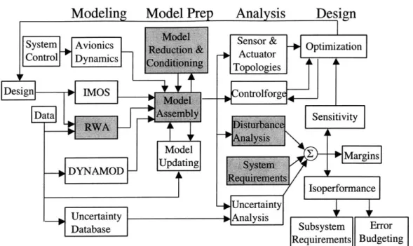
A suite of tools has been developed at the MIT Space Systems Laboratory for the pur-pose of completely analyzing the effects of disturbances on a spacecraft, and for examining the manner in which performances react to excitations. The collection of these tools is named DOCS, and describes all aspects of integrated modeling including Dynamics, Optics, Controls, and Structures (see Figure 1-1). The basic framework was developed by Gutier-rez [22] and consists of a series of MATLAB functions. Given a state-space structural system and any one of several types of disturbance models, these functions will determine the ex-pected performances, identify critical modes that contribute to performance degradation, determine the sensitivity of both modal and physical parameters to the disturbances, and follow model uncertainties through the analysis. The primary tool used in this work will be the disturbance analysis; along with determining whether or not a particular performance requirement is met, it also allows critical modes to be identified and can determine which disturbance inputs are providing the most energy to a mode. In this manner the DOCS functions provide more than just final performance results. Rather, they are designed for the purpose of iterative spacecraft design. By examining how the disturbances interact with a flexible spacecraft, and then by examining the sensitivities to determine which spacecraft parameters should be changed to most benefit the performance, exact design changes can be proposed and implemented.

Along with the basic disturbance and sensitivity functions, several other tools have been prepared at MIT to assist with spacecraft analysis and design. Identifying and modeling the disturbances is a key component of integrated modeling. The greatest contributor to spacecraft vibrations is expected to be the reaction wheels, used to slew and to hold the attitude of a spacecraft. Based on empirical data and analytical approximations, Master-son [28] has developed disturbance models that capture the key reaction wheel dynamics. These models will be used in the disturbance analysis of this work. Mallory [27] developed a controller tuning technique to improve upon baseline controllers. He also developed a method to determine which sensor/actuator combinations are suitable for a particular ap-plication, for example, system identification of a spacecraft's modeshapes. de Weck [15] has developed an iso-performance analysis to complement the sensitivity analysis. Whereas

Figure 1-1: An overview of the DOCS framework. Those areas used by or created by this

thesis are highlighted.

the sensitivities show how the performances can change based on variations in the modal or physical parameters, the iso-performance curves show how parameters can change while maintaining constant performance. This would be used at a higher level of design, after the requirements have been met, to trade performance errors between components in an effort to minimize costs (weight, monetary, or other).

One of the goals of the DOCS toolbox was to make it spacecraft-independent. It is designed as a generic tool that can be applied to any model framed in a state-space man-ner. Space observatories already examined include the original SIM model version 1.0 by

Gutierrez [22] and a low-fidelity model of NGST by de Weck [14]. This work will apply the

disturbance tools to a proposed NGST precursor mission named Nexus, as well as to the latest SIM model, version 2.2.

1.3

State Space Balancing and Reduction Routines

The critical step in working with large order models is reducing them to a more manageable size. For any given set of inputs and outputs, many of the elements in the state vector x can not be controlled and/or observed. Since these states do not affect the transfer function

0 0 0 500 500 500 1000 1000 1000 1500 1500 1500 2000 2000 2000 0 1000 2000 0 1000 2000 0 1000 2000 ns = 3222 ns = 4613904 ns = 99856

Figure 1-2: Structure of the SIM state-space A matrices: original sparse second order modal form (left) with 2148 states, fully populated balanced system (center), and fully populated reduced system with 316 states.

that describes the output for a given input, their presence in the system adds unnecessarily to the computational burden.

Several reduction routines have been proposed. Skelton has a series of papers that described Modal or Component Cost Analysis [23, 45, 46, 44]; a cost functional ranks each state, and those with the lowest costs can be removed. Another popular method is gramian balancing. This was first proposed by Moore [35], with extensions and modifications by Laub [25] and Gregory [19]. The gramians of a system describe the amount that states are controllable or observable. By transforming the system so that the gramians are equal, or balanced, the states are equally controllable and observable. The least controllable and observable can then be removed. As shown in Figure 1-2, balancing has the unfortunate result of turning a sparse matrix into one fully populated, but the reduction in number of states offsets this disadvantage. The fully populated balanced matrix is also better numerically conditioned than the sparse diagonal.

Despite its popularity, gramian balancing is difficult to implement on large-order models, if indeed the routine will run at all. Numerical ill-conditioning and the inversion of very small singular values can affect the accuracy of the final balanced model. Gregory recommends several approaches that can be taken, and Laub remarks on the difficulty of solving for the gramians. Neither of these papers explicitly provide any extensions on the basic algebraic transformation. Mallory [27] describes a method whereby large models can be balanced by removing some of the smallest singular values. This approach, termed balanced truncation, will be examined here. In order to improve the overall numerical quality of the system, several other steps will be discussed that improve numerical conditioning, or are required for gramian balancing. Once the system is balanced, additional reduction can still take

place. Examples of the resulting transfer functions will be provided.

1.4

Thesis Overview

This thesis describes the steps through a dynamic disturbance analysis, with emphasis on the model quality and conditioning, balancing, and reduction. An outline of the steps is provided in Figure 1-3. The chapter number that is associated with each block is given on the side. The first step, building a finite element (FE) model of a space observatory, involves taking the spacecraft design and modeling it using nodes, beams, plates, et cetera. This was done in all cases at the respective NASA facilities. The basic architecture of all three observatories, NGST, SIM, and Nexus, as well as a description of their FE models, is provided in Chapter 2. The mass M and stiffness K matrices that result are run through the basic dynamic eigenproblem in order to find the natural frequencies W and the struc-tural modeshapes <D. Some basic properties of the eigenproblem are provided in Chapter 3. Once damping is added to a system, the equations of motion can be cast into first or-der, state-space form, where the spacecraft dynamics, inputs and outputs are described by Equation 1.1.

As well as reviewing the eigenproblem, Chapter 3 also describes two popular linear algebra routines: the Singular Value Decomposition (SVD) and the Lyapunov equation. These routines are important for both the gramian balancing algorithm and for one type of disturbance analysis, so their basic properties and applications should be understood. In the case of the Lyapunov equation, a faster solver is also proposed that makes use of the structure of the A matrix.

Chapter 4 continues with the spacecraft analysis by performing some basic and necessary routines on the spacecraft model to prepare it for balancing. The idea of model quality management is emphasized here, where numerical conditioning, the nature of the inputs and outputs, and checks that can be run to track model quality are proposed. These steps are critical for the balancing of a large model.

A description of gramian balancing follows in Chapter 5. Because of the difficulties involved in inverting highly ill-conditioned matrices, balanced truncation is used. It is first necessary to define a tolerance for this truncation before the model can be balanced. The model is then reduced to a desired level; any one of several methods can be used to

determine the level of reduction. The balanced and reduced models can be compared to the original. If numerical difficulties either prevent the model from balancing or fail to produce an acceptable balanced model, a new truncation tolerance can be set and the balancing routine run again.

Once the model is successfully balanced and reduced, the integrated model can be assem-bled. This first involves preparing models that describe the disturbance sources. Reaction wheels will be used as the exclusive disturbance source for this analysis; an overview of their behavior and models is provided in Chapter 6. Models are prepared where wheel speed is treated as a stochastic random variable, and for actual discrete wheel speeds. At-titude control systems and optical control loops are added to the system in Chapter 7. For these analyses, no additional reduction is performed on the closed-loop models. As the flow diagram shows, however, ideally the entire closed loop system would be reduced. A first round of balancing and moderate reduction should be performed on the open loop system to provide numerical stability. The control loops can be closed, and the system reduced down to the desired model size.

A description and the implementation of the disturbance analysis is included in Chap-ter 7. The first disturbance analysis performed for the Nexus testbed is shown and the results are compared to its successor, NGST. This is followed by the first disturbance anal-ysis performed for the newest SIM model, version 2.2. Finally, in Chapter 8, the results of the SIM analysis are used to compare the version 2.2 model to the original SIM Version 1.0 model, whose analysis was performed in [22].

Chapter 9 concludes the thesis by describing the next steps in a dynamics analysis of a space observatory, and suggesting future work for the model quality control efforts.

Chapter 2

Chapter 3

Chapter 4

Chapter

5

Chapter 7

Chapter 8

Geometry Material Boundary Conditions 0-0c

Chapter 6

Chapter 2

Space Telescope Descriptions

As part of its Origins Program, NASA centers are currently developing several advanced space telescopes far more powerful and capable than the Hubble Space Telescope (HST) now in orbit. These spacecraft generally have more stringent pointing and wave front require-ments than HST and will rely upon technology still in development including lightweight mirrors, optical interferometry in space, and advanced optical controls, to meet these goals. Two of the space telescopes are being developed by NASA Goddard. The Next Gen-eration Space Telescope (NGST) is an infrared observatory currently scheduled to launch

around 2009. To alleviate some of the unknowns in the wave front control and mirror

technologies of this mission, Goddard engineers were concurrently developing the Nexus spacecraft'. Nexus was to have been a smaller space telescope that would be used as an on-orbit testbed. It has many of the same features as NGST, including lightweight mir-rors and a large sunshield, but its primary mission was to demonstrate technologies and verify models that will be used for NGST. The third spacecraft, the second true Origins spacecraft, is the Space Interferometry Mission (SIM) being designed at JPL. As the name implies, SIM is an optical interferometer, to be launched around 2006.

The spacecraft models were all acquired from the respective NASA centers, and all went through the reduction routine described in Chapter 5. A brief overview of each spacecraft's architecture and model is presented here.

2.1

Next Generation Space Telescope (NGST)

NGST is being planned as the next large observatory after Hubble. It was initially proposed by the HST and Beyond Committee to search in the "Dark Zone" of time between 100 mil-lion and 1 bilmil-lion years after the Big Bang [47]. Hubble's optics can resolve adolescent galaxies that formed several billion years after the Big Bang, and the Cosmic Background Explorer (COBE) produced images of the structure of the universe 300,000 years after the Big Bang. To observe the beginnings of galaxy formation between these times, however, a new spacecraft is needed.

The light from these early galaxies has been red-shifted because of their recession away from Earth, so their wavelengths are in the infrared. It was decided that an infrared telescope, cooled to below 50K with a primary mirror diameter of at least 4 meters, was required to examine this period of galaxy formation. The proposed orbit was around the L2 Lagrangian point, located on the line extending from the Sun through the Earth, on the anti-Sun side of the Earth (Figure 2-1). This distances the telescope from the gravity and atmospheric effects around Earth, plus it isolates the thermal effects of the Sun, Earth, and Moon to one side of the spacecraft.

-- --- 4

L3

Li

L2

-xL

Figure 2-1: Earth-Sun Lagrangian points. NGST is planned to orbit L2.

NASA Goddard began to design a possible architecture for this Next Generation Space Telescope, as did teams from Lockheed Martin and TRW/Ball Aerospace. Each of their designs is illustrated in Figure 2-2. The actual telescope will be designed and built by either Lockheed Martin or TRW, whoever wins the final down-select, scheduled for summer

2001. The purpose of the Goddard "Yardstick" design is to explore technical issues of the spacecraft including thermal design, disturbance sources, and wave front control. It also allows NASA engineers to develop requirements and error budgets, and to develop tools with which to examine the final contractor design. MIT was given this Yardstick model to examine. The initial DOCS analysis for the Yarkstick was performed by de Weck in [14].

(a) TRW/Ball Aerospace (b) Lockheed-Martin

T

(c) GSFC Yardstick

2.1.1

NGST Mission Architecture

Each of the three NGST designs employs a primary mirror (PM) over three times as large as Hubble's: 8 meters compared to 2.4 meters. Current plans are to launch NGST on an At-las IIAS-type booster [5]. Since such a large aperture would not fit within its launch shroud, the Yardstick primary mirror consists of 8 separate petals that would be stowed against the spacecraft during launch, and would deploy on orbit. They direct the science light to a secondary mirror located at the end of the long boom seen in Figure 2-2(c), which then directs the light to science instruments. These include a Near Infrared (NIR) instrument (wavelength A = 1 - 5pm), and a Mid Infrared (MIR) instrument (A > 10pm) [47].

The thermal environment of the optical components is one of the leading drivers in the spacecraft design. The Optical Telescope Assembly (OTA), which consists of the primary and secondary mirrors, along with the Integrated Science Instrument Module (ISIM), must remain cooled between 30-50K. To achieve this, NGST makes use of a large sunshield. The telescope remains in the cool shadow of this sunshield, while the bus instruments, and attitude and propulsion systems remain on the warm side. Mass and volume considerations require that the sunshield be lightweight; this also means that it will be very flexible, with a fundamental frequency around 0.3 Hz. This means that NGST will be much more dynamically active at low frequency than is HST. The MIR instrument will require further cooling to 6-8K. This will have to be achieved using active cryocoolers, despite the harmonic disturbances they transmit to the spacecraft.

The requirements for NGST are similar to Hubble (see Table 2.1); the challenge is that NGST is a much more flexible spacecraft . Line-of-sight (LOS) RMS relates to the pointing accuracy of the center of the science camera. The allowed jitter in the LOS is approximately 1/10 the resolution. For example, Hubble's resolution is 0.06 arcseconds [asec], and the LOS jitter requirement is 0.007 asec, or 7 milli-arcseconds (mas) [1]. The resolution for NGST will be 0.05 asec, with an associated jitter requirement of 5 mas (lo) [36]. The RMS wavefront error (WFE) is a measure of the different lengths traveled by two rays of light that enter the optics at the same time. The differences in pathlength can be caused by either static effects from aberrations in the mirror, quasi-static effects such as thermal warpage, or dynamics effects from vibrations. The WFE requirement for NGST in units of wavelength is A/14, or 0.157 pm at 2.2 microns wavelength.

In order to achieve this stability, active optical control of wavefront and pointing is required. Although optical control loops have been written for NGST, they are not used here. All of the NGST transfer functions that will be shown in this work are entirely in the open loop, so will not meet optical requirements. The purpose of the NGST disturbance analysis will be to determine the dynamic similarity of that observatory with Nexus. Since the Nexus model will not be closed loop either, the absence of a controller should not be a factor.

Table 2.1: Comparison of telescopes

Hubble NGST

Aperture [m] 2.4 8

Wavelength A [pm] 0.11 to 2.6 1 to 5

Resolution 0 [asec] 0.06 0.05

LOS requirement (RMS) [mas] 7 5

WFE Requirement (RMS) [pm] 0.0272 @ A=0.633 pm 0.157 @ A=2.2 pm

2.1.2 NGST Structural Finite Element Model

Several finite element (FE) models were created for NGST using JPL's Integrated Model-ing of Optical Systems (IMOS) modelModel-ing software. IMOS is a MATLAB based toolbox that builds a FE model using elements similar to those found in Nastran, but that allows the en-tire modeling process to remain in the MATLAB environment. Several models were created, including ngst8102, a 109 node model used in the previous MIT analysis [14]. This was

based on the ngst6033 model, with 995 nodes. A variation of this model, ngst603ss, was

used in place of the current Nexus model for disturbance studies, after Nexus underwent significant design changes. (explained in detail in Section 2.2). Ngst603ss includes an more detailed model of the sunshield, and as a result has many more low-frequency modes than its predecessors.

Ngst810 had been designed as a small model that could be worked with quite easily; few numerical problems were encountered with mathematical routines, and the turnaround time between analysis and design iteration could be reduced to hours. No additional

re-2

Created on 8/10/98

3

duction beyond simplifying the FE model was performed. The purpose of the balancing and reduction framework is to take a large state space representation of a spacecraft and reduce it to a size that allows fast and accurate results. For the purpose of testing these algorithms, a larger, more complex model is preferred to begin with. Ngst603ss better suits this purpose and will be used in subsequent chapters.

The ngst603ss model is shown in Figure 2-3. Most of the detail has gone into the OTA, with a simple Spacecraft Support Module (SSM) and ISIM comprised of several bar elements and concentrated masses. All of the reaction wheels are assumed to be collocated at the SSM

node (node #10291). For a disturbance analysis, this means that the individual disturbance

contributions from each wheel must be summed together, and the disturbances from the entire assembly applied at that single node (see Section 6.1). The cryocooler disturbances, three forces and one torque [14], act at the ISIM node where the MIR instrument would be

located (node #825).

Figure 2-3: ngst603ss FE Model

The first six modes of this model are rigid body modes, three translational and three rotational. The lowest flexible frequency is the first sunshield mode at 0.301 Hz, and most of the lower frequencies belong to sunshield modes [24]. Even these low modes are expected to drop in frequency with more realistic modeling of the sunshield [36]. The first bending mode of the Secondary Mirror support structure is at 4.9 Hz, and the first Primary Mirror

mode is at 5.1 Hz. These imply a much more flexible spacecraft than Hubble. Whereas Hubble is stiff enough such that it can rely entirely on its reaction wheels and rigid body controllers for optical pointing, NGST will require active optical actuators. Once the finite element model is prepared, an optics model is required to compute the optical performances.

2.1.3 NGST Optical Performance

The FE model of NGST provides nodal displacements. Although useful for determining strains or other displacement-dependent values, these do not provide much insight as to whether the spacecraft meets its optical requirements. These requirements were mentioned at the start of this subchapter: LOS jitter at or below 5 mas and RMS WFE of A/14.

The integrated model determines these optical metrics using linear combinations of nodal displacements and rotations from distinct nodes in the FE model that represent optical components (mirrors and optical instruments). These displacements and rotations are multiplied by the optical sensitivities to the movements. These sensitivities are found using MACOS (Modeling and Analysis for Controlled Optical Systems [10]), a ray-tracing program designed orignally at JPL. The wavefronts for representative light rays and the image centroid in the x- and y-axes are found as each reference node is perturbed one degree of freedom at a time. Two sensitivity matrices are thus computed, the centroid linear sensitivity matrix C/au and the wavefront linear sensitivity matrix &W/Ou, where u is a vector of generalized displacements from the reference nodes. These matrices allow calculation of wavefront and centroid RMS for a given u displacement vector.

C =Co + 0u

(2.1)

W =Wo+% ju

Redding, in Reference [40], provides an in-depth discussion of how the sensitivity matrices are computed.

The MACOS model provided for NGST uses eleven reference nodes: eight at the centers of each primary mirror (PM) petal plus one at the center of the entire PM structure (nodes #900-908), one at the secondary mirror (node #829) and one at the ISIM (node #825). These nodes are multiplied by the sensitivities to provide two centroid values for x and y in mas (so that OC/ou is a 2 x 11 matrix). They also provide 2440 WFE's in nanometers for a total of 2442 performance outputs (so that oW/ou is 2440 x 11). In the case of the WFE

sensitivity matrix, it should be noted that there are more columns than rows. This means that the columns in the matrix are not linearly independent, or the column space has not been reduced to its basis vectors [48]. Reference [13] provides a technique to reduce these matrices to a minimal basis using the singular value decomposition method. This allows

the same amount of information to be examined using smaller matrices.

Using the structural FE model along with the optics model, an integrated disturbance to performance model of NGST can be built. This model will be cast into state-space form and reduced by the techniques described in Chapter 5. After that the DOCS tools can be applied. Because of the technical challenges associated with NGST, Nexus was to have been used as a validation testbed. It will be described next.

2.2

Nexus

The Nexus space telescope was being developed by NASA Goddard as a precursor and tech-nology demonstrator mission for NGST, many of whose technologies have never been demon-strated in space. Several critical areas of uncertainty have been recognized for NGST [11]. They include fabrication and verification of the OTA, integration of the cryo-cooled instru-ments with the spacecraft thermal design, uncertain dynamics of the flexible sunshield, and wave front sensing and control (WFSC). To mitigate the risks associated with these uncer-tainties, Goddard engineers planned to build and fly Nexus. It would be a smaller telescope than NGST, but have many of the same features such as ultra-lightweight mirrors with image-based WFSC; a deformable mirror to compensate for wave front errors; a deployable, flexible sunshield; cryogenic actuators; and deployable optics (primary mirror).

Several flexible testbeds have already been flown in space, including the Middeck 0-gravity Dynamics Experiment (MODE) [8] and the Middeck Active Control Experiment (MACE) [30], both supported by MIT and launched in the Shuttle middeck. The Interfer-ometry Program Flight Experiments (IPEX I&II) free-flying testbeds were designed by JPL to study microdynamics of structures in space [26]. All of these were simple truss/boom structures. Nexus would be a full-fledged space telescope. The quality of its images would only have been on-par with Hubble, but the optics and spacecraft would be a technical validation of segmented infrared telescopes. The spacecraft would be instrumented with sensors and actuators (including accelerometers, shakers, heaters, and temperature gages),

to provide a complete dynamical and thermal characterization. This would allow, for ex-ample, verification of disturbance models (reaction wheels and cryocoolers) developed at

MIT.

2.2.1 Nexus Mission Architecture

Nexus went through several design changes as the mission was refined. Because all of the MIT analyses were performed on the older version of Nexus, also dubbed Horizon, this will be described first. The most current version, designed to more closely approximate NGST, will be described thereafter.

A partnership between the space science and Earth observing teams at Goddard led to the first Nexus design. The Earth Observing 3 (E03) Redeye mission was combined with Nexus to create the Horizon spacecraft (Figure 2-4). Initial plans were to launch Horizon from the Space Shuttle in LEO, and boost it to GEO so that the telescope would not be disturbed by the changing thermal environment of low Earth orbit. For stellar observation mode, Horizon was to have an accuracy of 2 asec and jitter of 1 asec. For Earth observing mode accuracy was to be 10 asec and jitter <0.5 asec [42].

Figure 2-4: Original Nexus/Horizon spacecraft (image from NASA Goddard Space Flight Cen-ter [38])

The primary mirror was made of three petals, similar in design to the eight petals on NGST. There was no sunshield, so the lowest structural mode was an order of magnitude higher in frequency than on NGST. Baffles covered by thermal blankets surrounded the entire OTA structure, and a door at the top of the baffles would be opened on-orbit to

allow light in. The lack of sunshield and rigid structure meant that Horizon would be dynamically stiffer than NGST. No cryo-coolers would be used, so their model validation and disturbance effects could not be examined. There would be four reaction wheels to maintain attitude and perform slews.

After funding difficulties were encountered, the E03 and Nexus missions were separated. Nexus was redesigned to look like a 1/3-scaled model of NGST (compare Figures 5 and 2-2). The architecture included a flexible sunshield and cryo-cooled instruments as described in the previous section. The three-petal primary mirror from Horizon was retained. Its

effective diameter was 2.8 meters. The baffles around the mirror were removed. The

requirements are less stringent than NGST: 15 asec pointing accuracy with 1 asec jitter over 1000 seconds [43], with only 0.5 asec jitter allocated to reaction wheel disturbances.

Figure 2-5: Current Nexus design (image from NASA Goddard Space Flight Center [11])

Plans were to launch Nexus to L2 on either a Delta II or Delta IV expendable booster. This provided the most similarity between the planned operating environment of NGST. Figure 2-6 shows the spacecraft in its stowed configuration, and gives an idea of how com-pactly NGST must be stowed.

2.2.2 Nexus Structural Finite Element Model

The only available FE model for Nexus was the original Nexus/Horizon model, displayed in Figure 2-7. This was used for an initial disturbance analysis described in Chapter 7. Later examinations of how the new Nexus design would behave used the ngst603 model.

The Horizon model contains 2681 nodes. The OTA nodes are particularly dense as the OTA model was built for thermal as well as dynamical analysis. This disparity in nodal

Figure 2-6: Nexus stowed configuration in a Delta II fairing. Note the stowed deployable primary mirror petal. (image from NASA Goddard Space Flight Center [11])

density is unwarranted for a dynamics solution, and the size of the corresponding M and K matrices would greatly increase the computational cost of a physical parameter sensitivity analysis. A smaller model was created by removing modes from the spacecraft. The number of modes was reduced from 2681 to 779 nodes. The FE pre-processor program FEMAP was used for this purpose. The primary mirror nodes after reduction are shown in Figure 2-8. The modal frequencies of the two models are plotted over each other in Figure 2-9. This shows that the dynamics remain fairly constant. The FEMAP model was then converted to

NASTRAN for a normal modes analysis. The MATLAB program nas2imos .m can be used

to convert the NASTRAN .dat file to IMOS format. From there the M and K matrices

can be built and used in the MATLAB environment.

Reaction wheel disturbances enter this model through four separate nodes (#'s 634, 640, 688, 694), representing each of the four reaction wheels. This differs from the NGST model with one node representing all of the reaction wheels. Nodes representing individual optical elements are included for the optics model.

The first flexible mode is at 1.9 Hz compared to 0.2 Hz for NGST. The structural differences will also be apparent in the disturbance analysis in Section 7.3.

Figure 2-7: Nexus/Horizon Finite Element Model

2.2.3 Nexus Optical Performance Metrics

A JPL-built MACOS optics model was used to compute performances for Nexus given the structural FE displacements. The initial disturbance analysis, using the 2681 node model, computed only three performance metrics using six degrees of freedom at each of four nodes. The node at the secondary mirror and three nodes from the primary mirror petals, one at the center of each, were multiplied by the optical sensitivities to the motions of those points. The performance metrics were centroid jitter in both the x- and y-axes in meters, and the WFE of only one ray in meters.

Note that centroid jitter is given in units of length and not angle in the sky. To convert to arcseconds of angle requires the plate scale of the CCD detector, missing here. The plate scale specifies the angle in the sky that each pixel can view, and since the jitter is actually the movement of a guide star or extended source image over the pixels in the plane perpendicular (approximately) to the incoming light, it can be described using units of length. In order to specify the pointing stability of the telescope however, the movement of the pixels is converted to the angle affected by that movement.

A more complete analysis requires the plate scale and use of more than one ray for a WFE analysis. The integrated model can still be used to show general behavior of the

Figure 2-8: Primary Mirror of the Reduced Nexus/Horizon FEM

Nexus/Horizon model, and can compare the dynamics of Nexus/Horizon with those of NGST. Since the full-order model will be used in the disturbance analysis of Chapter 7, the integrated model will not be taken through the reduction routines of Chapter 5.

The next and final spacecraft considered will is a visual interferometer, the Space Inter-ferometry Mission.

2.3

Space Interferometry Mission (SIM)

The final spacecraft examined is the Space Interferometry Mission being designed at JPL (Figure 2-10). SIM will be the first space telescope to employ optical interferometry for precision astrometry, or the measurement of the exact position of stellar objects. It will be able to detect the position of a stellar object to about 4 pas (micro-arcseconds), or about a billionth of a degree [7, 49]. This will give scientists a far greater understanding about the formation of planets and galaxies. For example, by detecting the wobble of stars relative to reference stars, SIM will be able to detect extra-solar planets smaller than those found thus far; it should even be able to determine the existence of terrestrial planets only several times larger than Earth orbiting nearby stars [49]. It can use parallax, or triangulation from observing locations on opposite sides of the sun, to determine the distance to any star in

10 4) U-0 0 0 *~ L2681odesj 100 77 nodes 0 10 20 30 40 50 60 70 80 90 100 Mode number

Figure 2-9: Comparison of modal frequencies between high- and low-fidelity Nexus/Horizon models

our galaxy brighter than 1 8th magnitude. Observations of distant galaxies will enable more

precise estimates of the Hubble constant and the age of the universe.

Not only will SIM return valuable scientific data, but it will also demonstrate space-based interferometry for a new generation of telescopes. For example, the Terrestrial Planet Finder (TPF) [37] will rely on destructive interference of science light to block the light of a star, allowing the habitable range for terrestrial planets to be observed. TPF and its kin may rely on light gathered from multiple spacecraft moving in formation. SIM will still use telescopes located on a single spacecraft.

2.3.1 SIM Mission Architecture

At its core SIM will consist of a 10 meter baseline Michelson interferometer [7, 6]. Eight tele-scopes, called siderostats, will be placed linearly along the main structure of the spacecraft, the Precision Support Structure (PSS). The light from any combination of two telescopes can make an interferometer. The collected light is passed through a switchyard to determine which light beams will be combined. Optical delay lines are used to ensure the distances traveled by two coplanar light rays are equal. The light is finally directed to beam com-biners for interference. The furthest two telescope bays will nominally make up the science