HAL Id: hal-01699185
https://hal.archives-ouvertes.fr/hal-01699185
Submitted on 16 May 2018
HAL is a multi-disciplinary open access
archive for the deposit and dissemination of
sci-entific research documents, whether they are
pub-lished or not. The documents may come from
teaching and research institutions in France or
abroad, or from public or private research centers.
L’archive ouverte pluridisciplinaire HAL, est
destinée au dépôt et à la diffusion de documents
scientifiques de niveau recherche, publiés ou non,
émanant des établissements d’enseignement et de
recherche français ou étrangers, des laboratoires
publics ou privés.
An optimal reciprocally convex inequality and an
augmented Lyapunov–Krasovskii functional for stability
of linear systems with time-varying delay
Xian-Ming Zhang, Qing-Long Han, Alexandre Seuret, Frédéric Gouaisbaut
To cite this version:
Xian-Ming Zhang, Qing-Long Han, Alexandre Seuret, Frédéric Gouaisbaut.
An optimal
re-ciprocally convex inequality and an augmented Lyapunov–Krasovskii functional for stability
of linear systems with time-varying delay.
Automatica, Elsevier, 2017, 84, pp.221 - 226.
An optimal reciprocally convex inequality and a new Lyapunov-Krasovskii functional for
stability analysis of linear systems with time-varying delay
IXian-Ming Zhanga, Qing-Long Hana,∗, Alexandre Seuretb, Fr´ed´eric Gouaisbautc
aSchool of Software and Electrical Engineering, Swinburne University of Technology, Hawthorn, Melbourne, VIC 3122, Australia bLAAS-CNRS, Universit´e de Toulouse, CNRS, Toulouse, France
cUniv. de Toulouse, UPS, LAAS, F-31400, Toulouse, France
Abstract
This paper is concerned with stability of a linear system with a time-varying delay. First, an optimal reciprocally convex inequality is proposed. Compared with the extended reciprocally convex inequality recently reported, the optimal reciprocally convex inequality not only provides an optimal bound for the reciprocally convex combination, but also introduces less slack matrix variables. Second, a new Lyapunov-Krasovskii functional is tailored for the use of auxiliary function-based integral inequality. Third, based on the optimal reciprocally convex inequality and the new Lyapunov-Krasovskii functional, a stability criterion is derived for the system under study. Finally, two well-studied numerical examples are given to show that the obtained stability criterion can produce a larger upper bound of the time-varying delay than some existing methods.
Keywords: Time-delay systems, stability, reciprocally convex inequality, Lyapunov-Krasovskii functional.
1. Introduction
Consider the system with a time-varying delay described by
x(˙x(t)θ) = ϕ(θ), θ ∈ [−h= Ax(t) + Adx(t− h(t))M, 0], (1) where x(t) ∈ Rn is the system state; A and Ad are real n× n
constant matrices; h(t) is the time-varying delay satisfying 0≤ h(t) ≤ hM, dm≤ ˙h(t) ≤ dM< ∞ (2)
with hM, dmand dMknown scalars; andϕ(θ) is an initial
condi-tion. To begin with, for simplicity of presentation, we denote ρ1(t) := ∫t−h(t) t−hM x(s) hM−h(t)ds, ρ2(t) := ∫t−h(t) t−hM (t−h(t)−s)x(s) (hM−h(t))2 ds ρ3(t) := ∫t t−h(t) x(s) h(t)ds, ρ4(t) := ∫t t−h(t) (t−s)x(s) h2(t) ds. (3)
The Lyapunov-Krasovskii functional method plus integral inequalities is regarded as a powerful tool for deriving a maxi-mum upper bound hMthat the system (1) can tolerate and
main-tain stability (He et al. , 2007; Gu & Liu , 2009; Gu , 2013; Xu et al. , 2015). This method has gained increasing attention especially since the Jensen integral inequality is improved by the Wirtinger-based integral inequality (Seuret & Gouaisbaut , 2013), and much effort has been made in seeking less conser-vative stability criteria for the system (1), e.g. Zhang & Han (2015), Zhang et al. (2016), Zeng et al. (2015a), Kim (2016).
IThis paper was not presented at any IFAC meeting.
∗Corresponding author: Qing-Long Han, Tel.: +61 3 9214 3808; E-mail: qhan@swin.edu.au
It should be mentioned that the Wirtinger-based integral in-equality is further improved by the auxiliary function-based integral inequality (Seuret & Gouaisbaut , 2015; Park et al. , 2015). However, it is found that, if taking some Lyapunov-Krasovskii functional, the stability criterion based on the aux-iliary function-based integral inequality may be of the same conservatism as the one based on the Wirtinger-based inte-gral inequality. To make it clear, we take the proof of Theo-rem 7 in Seuret & Gouaisbaut (2013) for example, where the Lyapunov-Krasovskii functional is chosen as
˜
V(xt, ˙xt)= ˜xT(t)P ˜x(t)+ ˜V1(t, xt)+ V2(t, ˙xt) (4)
where ˜x(t) := col{x(t), h(t)ρ3(t), (hM−h(t))ρ1(t)}, and ˜ V1(t, xt)= ∫ t t−h(t) xT(s)Qx(s)ds+ ∫ t t−hm xT(s)S x(s)ds (5) V2(t, ˙xt)= ∫ t t−hM ∫ t θ ˙x T(s)R ˙x(s)dsdθ (6)
Applying the Wirtinger-based integral inequality, it is proven that (Seuret & Gouaisbaut , 2013)
˙˜V(xt, ˙xt)≤ ξT1(t)Φ(h(t), ˙h(t))ξ1(t), (7) whereξ1(t) = col{x(t), x(t − h(t)), x(t − hM), ρ3(t), ρ1(t)} with ρ1(t) and ρ3(t) defined in (3), and Φ(h(t),˙h(t)) is defined in Seuret & Gouaisbaut (2013). However, use the auxiliary function-based integral inequality (i.e. Lemma 1 on the next page) and the reciprocally convex approach (Park et al. , 2011) to get
whereξ2(t) := col{x(t−h(t))− x(t−hM)−6ρ1(t)+12ρ2(t), x(t)−
x(t− h(t)) − 6ρ3(t)+ 12ρ4(t)} with ρ2(t) andρ4(t) defined in (3), andΨ := 1
hM[
5R ˜S
˜
ST 5R] ≥ 0. Denote ζ1(t) = col{ξ1(t), 0, 0}, ζ2(t) = col{ξ1(t), ρ4(t), ρ2(t)} and Γ = [0 II−I 0 −6I 0 12I 0−I 0 −6I 0 12I].
Then (8) can be rewritten as
˙˜V(xt, ˙xt)≤ ζ1T(t)diag{Φ(h(t), ˙h(t)), −I}ζ1(t)−ζ2T(t)Γ
TΨΓζ
2(t) (9) Notice that ζ1(t) andζ2(t) are linearly independent sinceζ1(t) does not include the vectorsρ2(t) andρ4(t). Thus, the stability criteria derived from (7) and (9) both can be given by the same form asΦ(h(t), ˙h(t)) < 0 due to Ψ ≥ 0. Therefore, the use of the auxiliary function-based integral inequality may not reduce the conservatism of the obtained stability criterion.
From the above analysis, it is clear to see that, in order to derive less conservative stability criteria, one should construct a proper Lyapunov-Krasovskii functional such that the corre-sponding vectorζ1(t) is linearly dependent on the vectorζ2(t) in (9). To construct such a Lyapunov-Krasovskii functional is the first motivation of the study.
On the other hand, the reciprocally convex approach is wide-ly used in the stability anawide-lysis of linear systems with time-varying delay. It is because, as stated in Park et al. (2011), the reciprocally convex approach can produce stability criteri-a with less decision vcriteri-aricriteri-ables while the conservcriteri-atism will not be increased. Recently, the reciprocally convex inequality in Park et al. (2011) is extended in Seuret & Gouaisbaut (2016) by introducing four slack matrix variables. Although the ex-tended reciprocally convex inequality is helpful for deriving a less conservative stability condition, the introduction of four slack matrix variables undoubtedly increases the computation complexity of the obtained stability criterion. How to reduce the slack matrix variables of the extended reciprocally convex inequality is a significant issue, which is the second motivation of the study.
In this paper, we focus on the stability analysis of linear sys-tems with time-varying delay described by (1). First, an optimal reciprocally convex inequality is proposed, which provides an optimal bound for the reciprocally convex combination, while less slack matrix variables are introduced if compared with the extended reciprocally convex inequality (Seuret & Gouaisbaut , 2016). Second, a new Lyapunov-Krasovskii functional is tai-lored for the use of the auxiliary function-based integral in-equality. On the one hand, the termsρ2(t) andρ4(t) appear in the derivative of the Lyapunov-Krasovskii functional, which mean-s that the auxiliary function-bamean-sed integral inequality can be used to formulate less conservative stability criteria; and on the other hand, the quadratic ˜xT(t)P ˜x(t) in (4) is deleted. Instead,
˜
V1(t, xt) in (5) is augmented so that the relationship between
ρj(t) ( j = 1, · · · , 4) and the other vectors is enhanced in the
derivative of the Lyapunov-Krasovskii functional. Third, the optimal reciprocally convex inequality and the new Lyapunov-Krasovskii functional are employed to derive a new stability criterion for the system (1), whose effectiveness is demonstrat-ed through two well-usdemonstrat-ed numerical examples.
Notations:λmax(Q) (λmin(Q)) stands for the maximum (min-imum) eigenvalue of the matrix Q; Sym{A} = A + AT.
To end this section, we introduce some lemmas, which are useful in the stability analysis.
Lemma 1. (Seuret& Gouaisbaut , 2015; Park et al. , 2015).
For any n× n constant real matrix R > 0, two scalars r1 and
r2with r2 > r1, and a vector-valued functionω : [r1, r2]→ Rn
such that the integrations below are well defined, then
∫ r2 r1 ˙ ωT(s)R ˙ω(s)ds ≥ 1 r2−r1ζ T(r 1, r2) ˜Rζ(r1, r2) (10)
where ˜R := diag{R, 3R, 5R} and ζ(r1, r2) := col{υ0, υ1, υ2} with υ0:= ω(r2)− ω(r1) and υ1:=ω(r2)+ ω(r1)− 2 r2−r1 ∫r2 r1 ω(s)ds υ2:=υ0−r6 2−r1 ∫r2 r1 ω(s)ds+ 12 (r2−r1)2 ∫r2 r1(r2−s)ω(s)ds (11)
Lemma 2. (Kim , 2016). For a given quadratic functionℓ(s) =
a2s2 + a1s+ a0, where ai ∈ R (i = 0, 1, 2), if the following
inequalities hold
(i).ℓ(0) < 0; (ii). ℓ(h) < 0; (iii). − h2a2+ ℓ(0) < 0 (12)
one hasℓ(s) < 0 for ∀s ∈ [0, h].
Lemma 3. (Fridman , 2014). The system (1) is asymptotically
stable if the exists a quadratic Lyapunov-Krasovskii functional V(t, ϕ, ˙ϕ) such that for some εi> 0 (i = 1, 2, 3)
ε1∥ϕ(0)∥2≤ V(t, ϕ, ˙ϕ) ≤ ε2∥ϕ∥2W ˙ V(t, ϕ, ˙ϕ) ≤ −ε3∥ϕ(0)∥2 where∥ϕ∥2 W= ∥ϕ(0)∥ 2+∫0 −hM∥ϕ(s)∥ 2ds+∫0 −hM∥ ˙ϕ(θ)∥ 2dθ. 2. Main results
In this section, we will present our main results. An optimal reciprocally convex inequality and a new Lyapunov-Krasovskii functional are introduced, based on which a novel stability cri-terion is derived for the system (1).
2.1. An optimal reciprocally convex inequality
Recently, the reciprocally convex inequality proposed in Park et al. (2011) is extended by introducing some slack ma-trix variables, which is given as follows.
Lemma 4. (Seuret& Gouaisbaut , 2016). Let R1, R2 ∈ Rm×m
be real symmetric positive definite matrices andϖ1, ϖ2 ∈ Rm
and a scalarα ∈ (0, 1). If there exist real symmetric matrices X1, X2∈ Rm×mand real matrices Y1, Y2∈ Rm×msuch that
[ R1−X1 Y1 YT 1 R2 ] ≥ 0, [ R1 Y2 YT 2 R2−X2 ] ≥ 0 (13)
the following inequality holds F (α) := 1αϖT 1R1ϖ1+ 1 1−αϖ T 2R2ϖ2≥ G (X1, X2) (14) G (X1, X2) := ϖT1[R1+(1−α)X1]ϖ1+ϖT2(R2+αX2)ϖ2 + 2ϖT 1[αY1+ (1 − α)Y2]ϖ2 (15) 2
Lemma 4 presents a general lower boundG (X1, X2) for the reciprocally convex combinationF (α) by introducing four s-lack matrix variables, which bring additional degree of freedom if compared with the one in Park et al. (2011). However, more slack matrix variables usually lead to high computation com-plexity. The following analysis gives an optimal lower bound forF (α) from the set {G (X1, X2)|(X1, X2) satisfies (13)}. Theorem 1. LetR1, R2∈ Rm×mbe real symmetric positive
def-inite matrices andϖ1, ϖ2 ∈ Rmand a scalarα ∈ (0, 1). Then
for any Y1, Y2∈ Rm×m, the following inequality holds
F (α) ≥ ϖT 1[R1+(1−α)(R1− Y1R−12 Y T 1)]ϖ1 + ϖT 2[R2+α(R2− Y2TR−11 Y2)]ϖ2 + 2ϖT 1[αY1+ (1 − α)Y2]ϖ2 (16) Proof. Since R1> 0 and R2> 0, the matrix inequalities in (13) are equivalent to, respectively,
R1− X1− Y1R−12 Y T 1 ≥ 0, R2− X2− Y2TR1−1Y2 ≥ 0 (17) Denote X10 = R1− Y1R−12 Y T 1 and X20 = R2− Y2TR−11 Y2. Then it follows from (17) that X10 ≥ X1 and X20 ≥ X2, which leads toG (X10, X20)≥ G (X1, X2), whereG (X1, X2) is defined in (15). Since (X10, X20) satisfies (13), by Lemma 4, one obtains
F (α) ≥ G (X10, X20)≥ G (X1, X2) (18) which completes the proof.
Remark 1. Compared with Lemma 4, Theorem 1 provides an optimal lower bound G (X10, X20) for the reciprocally convex combinationF (α). It is worth pointing out that the slack ma-trix variables X1 and X2 in (13) are removed from Theorem 1. Moreover, if one sets Y1 = Y2 = S , it is easy to show that
G (X10, X20) is greater thanϖT1R1ϖ1+ 2ϖT1Sϖ2 + ϖT2R2ϖ2, which is originally proposed in Park et al. (2011).
Remark 2. In Seuret & Gouaisbaut (2016), it is suggested to reduce the number of decision variables in Lemma 4 by impos-ing a constraint X1 = X2 on X1 and X2. However, in the case where the dimensions ofR1andR2are not compatible, one can-not set X1= X2; and in the case whereR1= R2, the constraint
X1 = X2only makes the lower boundG (X1, X1) deviate away from the optimal oneG (X10, X20) due to that, in most cases, X10 is not equal to X20even though one sets Y1= Y2.
2.2. An augmented Lyapunov-Krasovskii functional
In this section, we introduce a Lyapunov-Krasovskii func-tional candidate as V(t, xt, ˙xt)= V1(t, xt)+ hMV2(t, ˙xt) (19) where xt := x(t + θ), θ ∈ [−hM, 0]; V2(t, ˙xt) is defined in (6); and V1(t, xt) := ∫ t t−h(t) ηT 1(t, s)Q1η1(t, s)ds + ∫ t−h(t) t−hM ηT 2(t, s)Q2η2(t, s)ds (20) where Q1> 0, Q2> 0 and R > 0 are to be determined, and
η1(t, s) := col { ˙x(s), x(s), η0(t), ∫s t−h(t)x(θ)dθ } η2(t, s) := col { ˙x(s), x(s), η0(t), ∫s t−hMx(θ)dθ } η0(t) := col {x(t), x(t − h(t)), x(t − hM)}
It is not difficult to verify that there exist two constants c1 > 0 and c2> 0 such that
c1∥xt(0)∥22≤ V(t, xt, ˙xt)≤ c2∥xt∥2W. (21)
In fact, denoteϵ0= min{λmin(Q1),λmin(Q2)}. Then
V1(t, xt)≥ ∫ t t−h(t) ϵ0xT(t)x(t)ds+ ∫ t−h(t) t−hM ϵ0xT(t)x(t)ds = hMϵ0xT(t)x(t), c1xT(t)x(t) (22) On the other hand, denoteϵ1= max{λmax(Q1),λmax(Q2)}. Then
V1(t, xt)≤ ϵ1 ∫ t t−hM [ ∥ ˙x(s)∥2 2+∥x(s)∥ 2 2+∥η0(t)∥22 ] ds + ϵ1 ∫ t t−h(t) ∫ s t−h(t) ∥xT(θ)∥ 2dθ ∫ s t−h(t) ∥x(θ)∥2dθds + ϵ1 ∫ t−h(t) t−hM ∫ s t−hM ∥xT(θ)∥ 2dθ ∫ s t−hM ∥x(θ)∥2dθds ≤ ϵ1 ∫ t t−hM [ ∥ ˙x(s)∥2 2+3∥x(s)∥ 2 2 ] ds+ ϵ1hM∥xt(0)∥22 + ϵ1 ∫ t t−h(t) hM ∫ t t−hM ∥x(θ)∥2 2dθds + ϵ1 ∫ t−h(t) t−hM hM ∫ t t−hM ∥x(θ)∥2 2dθds ≤ ϵ1hM∥xt(0)∥22+ϵ1 ∫ t t−hM [ ∥ ˙x(s)∥2 2+(h 2 M+3)∥x(s)∥ 2 2 ] ds V2(t, ˙xt)≤ hMλmax(R) ∫ t t−hM ∥ ˙x(s)∥2 2ds which follows that
V(t, xt, ˙xt)≤ ϵ1hM∥xt(0)∥22+(h 2 M+3)ϵ1 ∫ t t−hM ∥x(s)∥2 2ds + [h2 Mλmax(R)+ϵ1] ∫ t t−hM ∥ ˙x(s)∥2 2ds
Thus, there exists a constant c2:= max{ϵ1hM, h2Mλmax(R)+ϵ1, (h2
M+ 3)ϵ1}, such that V(t, xt)≤ c2∥xt∥
2
W.
Compared with some existing Lyapunov-Krasovskii func-tionals, e.g. (4) and He et al. (2005), Seuret & Gouaisbaut (2013), Kim (2016), V(t, xt) in (19) has the following
char-acteristics:
i) The quadratic term, say xT(t)Px(t) or ˜xT(t)P ˜x(t) in (4), is
deleted. Instead, an augmented integral term V1(t, xt) is
and x(t− hM) are closely coupled by the matrices Q1and
Q2. Such coupling can enhance the relationship between
x(t) and the other delayed state vectors in the derivative of V1(t, xt); and
ii) Taking the time-derivative of V1(t, xt) yields two important
integrals ρ2(t) andρ4(t), which enable us to employ the integral inequality (10) to derive less conservative stability conditions.
2.3. A new stability criterion
In this section, based on Theorem 1 and the Lyapunov-Krasovskii functional (19), we establish and state a novel delay-dependent stability criterion for the system (1).
Proposition 1. For given scalars hM, dm and dM, the system
(1) is asymptotically stable if there exist real matrices Q1 > 0,
Q2 > 0, R > 0, Y1 and Y2 with appropriate dimensions such
that [ Υ1(0, d)|d=dm,dMΓ T 2Y T 2 Y2Γ2 − ˜R ] < 0, [ Υ(hM, d)|d=dm,dMΓ T 1Y1 Y1TΓ1 − ˜R ] < 0 (23) [ [−h2MG0(d)+ Υ1(0, d)]|d=dm,dM Γ T 2Y T 2 Y2Γ2 − ˜R ] < 0 (24)
where ˜R= diag{R, 3R, 5R} and
Υ1(h(t), ˙h(t)) := [C11+h(t)C12]TQ1[C11+h(t)C12] + h2 MC T 0RC0−C5TQ2C5−(1−˙h(t))C2TQ1C2−(2−α)ΓT1R˜Γ1 + (1−˙h(t))[C41+(hM− h(t))C42]TQ2[C41+(hM− h(t))C42] + Sym{DT 1Q1[C30+ h(t)C31+ h2(t)C32] } + Sym{DT 2Q2[C60+(hM−h(t))C61+(hM−h(t))2C62] } − (1+α)ΓT 2R˜Γ2−Sym { ΓT 1[αY1+ (1 − α)Y2]Γ2 } (25) G0(˙h(t)) := C12TQ1C12+(1−˙h(t))C42TQ2C42 + Sym{DT 1Q1C32+D2TQ2C62 } (26) whereC0:= Ae1+ Ade2,α = (hM− h(t))/hMand C11:= col{C0, e1, e1, e2, e3, 0}, C12:= col{0, 0, 0, 0, 0, e6} C2:= col{e8, e2, e1, e2, e3, 0}, C30 := col{e1− e2, 0, 0, 0, 0, 0} C31:= col{0, e6, e1, e2, e3, 0}, C32 := col{0, 0, 0, 0, 0, e7} C41:= col{e8, e2, e1, e2, e3, 0}, C42 := col{0, 0, 0, 0, 0, e4} C5:= col{e9, e3, e1, e2, e3, 0}, C60 := col{e2− e3, 0, 0, 0, 0, 0} C61:= col{0, e4, e1, e2, e3, 0}, C62 := col{0, 0, 0, 0, 0, e5}
D1:= col{0, 0, C0, (1 − ˙h(t))e8, e9, (˙h(t) − 1)e2}
D2:= col{0, 0, C0, (1 − ˙h(t))e8, e9, −e3}
Γ1:= col{e2−e3, e2+e3−2e4, e2−e3−6e4+12e5} Γ2:= col{e1−e2, e1+e2−2e6, e1−e2−6e6+12e7}
with ei(i= 1, 2, · · · , 9) being the i-th n × 9n block-row vectors
of the 9n× 9n identity matrix.
Proof. Taking the time derivative of V(t, xt) in (19) along with
the trajectory of the system (1) yields ˙ V(t, xt)= ˙V1(t, xt)+ hMV˙2(t, xt) (27) where ˙ V1(t, xt)= ηT1(t, t)Q1η1(t, t)−ηT2(t, t − hM)Q2η2(t, t − hM) − (1 − ˙h(t))ηT 1(t, t − h(t))Q1η1(t, t − h(t)) + (1 − ˙h(t))ηT 2(t, t − h(t))Q2η2(t, t − h(t)) + ∫ t t−h(t) 2ηT1(t, s)Q1∂η 1(t, s) ∂t ds + ∫ t−h(t) t−hM 2ηT2(t, s)Q2 ∂η2(t, s) ∂t ds (28) hMV˙2(t, xt)= h2M˙x T(t)R ˙x(t)− h M ∫ t t−hM ˙xT(s)R ˙x(s)ds (29) For simplicity, denote
ξ(t) := col{x(t), x(t − h(t)), x(t − hM), ρ1(t), ρ2(t), ρ3(t), ρ4(t), ˙x(t−h(t)), ˙x(t−hM)} (30)
whereρj(t) ( j = 1, 2, 3, 4) are defined in (3). Then one has
˙x(t)=C0ξ(t), and η1(t, t) = (C11+h(t)C12)ξ(t), η1(t, t − h(t)) = C2ξ(t), η2(t, t−h(t)) = [C41+(hM−h(t))C42]ξ(t), η2(t, t−hM)= C5ξ(t), ∫ t t−h(t) 2ηT1(t, s)Q1∂η 1(t, s) ∂t ds = 2ξT(t)DT 1Q1 [ C30+ h(t)C31+ h2(t)C32 ] ξ(t), (31) ∫ t−h(t) t−hM 2ηT2(t, s)Q2∂η 2(t, s) ∂t ds= 2ξT(t)D2TQ2 ×[C60+ (hM− h(t))C61+ (hM− h(t))2C62 ] ξ(t). (32) DenoteI (t) := hM ∫t t−hM ˙x T(s)R ˙x(s)ds. Then I (t) = hM ∫ t−h(t) t−hM ˙xT(s)R ˙x(s)ds+ hM ∫ t t−h(t) ˙xT(s)R ˙x(s)ds Applying Lemma 1 yields
hM ∫ t−h(t) t−hM ˙xT(s)R ˙x(s)ds≥ 1 α(Γ1ξ(t))TR(˜ Γ1ξ(t)) hM ∫ t t−h(t) ˙xT(s)R ˙x(s)ds≥ 1 1− α(Γ2ξ(t)) TR(˜ Γ 2ξ(t))
whereα = (hM− h(t))/hM. Thus, apply (16) withR1= R2= ˜R, ϖ1= Γ1ξ(t) and ϖ2= Γ2ξ(t) to obtain I (t) ≥ ξT(t)[Υ 0−(1−α)ΓT1Y1R˜−1Y1TΓ1−αΓT2Y T 2R˜−1Y2Γ2 ] ξ(t) Υ0:=(2−α)ΓT1R˜Γ1+(1+α)ΓT2R˜Γ2+S ym { ΓT 1[αY1+(1−α)Y2]Γ2 } To sum up, one has that
˙
V(t, xt)≤ ξT(t)[Υ1(h(t), ˙h(t)) + Υ2(h(t))]ξ(t) (33) 4
Table 1: The maximum admissible upper bound hM for d= −dm = dM for Example 1 Method\ d 0.1 0.5 0.8 NoDVs Kim (2016) 4.753 2.429 2.183 27n2+4n Zeng et al. (2015) 4.788 3.055 2.615 65n2+11n Proposition 1 4.910 3.233 2.789 54.5n2+6.5n
whereΥ1(h(t), ˙h(t)) is defined in (25), and Υ2(h(t)) := (1−α)ΓT1Y1R˜−1Y1TΓ1+αΓT2Y
T
2R˜−1Y2Γ2 Notice that
Υ1(h(t), ˙h(t))+Υ2(h(t))=h2(t)G0(˙h(t))+h(t)G1(˙h(t))+G2(˙h(t)) whereG0(˙h(t)) is defined in (26);G1(˙h(t)) andG2(˙h(t)) are some proper real symmetric matrices irrespective of h(t). Let us con-sider the quadratic functionχT[Υ1(h(t), ˙h(t))+Υ2(h(t))]χ as
χT[Υ
1(h(t), ˙h(t))+Υ2(h(t))]χ = a2h2(t)+ a1h(t)+ a0 (34) where a0= χTG2(˙h(t))χ, a1= χTG1(˙h(t))χ and a2= χTG0(˙h(t))χ with χ ∈ R9n. If the linear matrix inequalities in (23) and (24) are satisfied, applying Lemma 2 and the Schur comple-ment yieldsχT[Υ
1(h(t), ˙h(t))+Υ2(h(t))]χ < 0 for h(t) ∈ [0, hM]
and ˙h(t) ∈ [dm, dM]. Letχ = ξ(t). Then one has ˙V(t, xt) ≤
ξT(t)[Υ
1(h(t), ˙h(t)) + Υ2(h(t))]ξ(t) < 0 for h(t) ∈ [0, hM] and
˙h(t)∈ [dm, dM]. Thus, applying Lemma 3, one can draw a
con-clusion that the system (1) is asymptotically stable.
Remark 3. Proposition 1 presents a novel stability criteria based on the new Lyapunov-Krasovskii functional. From the proof, it is clear that in the estimation of ˙V(t, xt), Theorem 1
and Lemma 1 play a key role in deriving a tight upper bound for ˙V(t, xt). It is worth pointing out that Lemma 2 proposed in
Kim (2016) provides a useful method to deal with the quadratic function (34) on the time-varying delay h(t). Simulation result-s in the next result-section result-show that Proporesult-sition 1 can produce leresult-sresult-s conservative results than some existing approaches.
3. Numerical examples
Example 1. Consider the system(1) with
A= [ −2 0 0 −0.9 ] , Ad= [ −1 0 −1 −1 ] (35)
and the delay h(t) is time-varying satisfying (2).
For comparison with some existing approaches, we calcu-late the maximum admissible upper bound hM for different
d = −dm= dM. For d ∈ {0.1, 0.5, 0.8}, applying the
approach-es in Kim (2016), Zeng et al. (2015) and Proposition 1, the obtained results are given in Tab. 1. Moreover, the number of decision variables (NoDVs) involved in solving the correspond-ing linear matrix inequalities is also listed in Tab. 1. From this
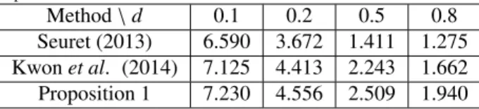
Table 2: The maximum admissible upper bound hM for d = −dm = dM for
Example 2
Method\ d 0.1 0.2 0.5 0.8
Seuret (2013) 6.590 3.672 1.411 1.275
Kwon et al. (2014) 7.125 4.413 2.243 1.662
Proposition 1 7.230 4.556 2.509 1.940
table, one can see clearly that Proposition 1 delivers some larg-er upplarg-er bounds hM for the time-varying delay h(t) than those
by Kim (2016) and Zeng et al. (2015). It should be mentioned that the number of decision variables required in Proposition 1 is smaller than that in Zeng et al. (2015).
Example 2. Consider the system(1) with
A= [ 0 1 −1 −1 ] , Ad = [ 0 0 0 −1 ] (36)
and the delay h(t) is time-varying satisfying (2).
For this example, in Seuret & Gouaisbaut (2013) and Kwon et al. (2014), the maximum admissible upper bound hM
of the time-varying delay h(t) is calculated for d = −dm =
dM ∈ {0.1, 0.2, 0.5, 0.8} and the obtained results are listed in
Tab. 2. However, applying Proposition 1 yields some larger up-per bounds hM, which are also given in this table. It is clear to
see that for d= 0.8, the maximum upper bound hMis improved
by 16.73% and 52.16%, respectively, if compared with the ones in Kwon et al. (2014) and Seuret & Gouaisbaut (2013).
4. Conclusion
Stability of linear systems with time-varying delay has been revisited in this paper. By introducing an optimal reciprocally convex inequality and a new Lyapunov-Krasovskii functional, a novel stability criterion has been derived for the system under study. It has been shown that through two well-used numerical examples the obtained stability criterion can deliver larger up-per bounds for the time-varying delay than some existing ones.
Acknowledgements
This work was supported in part by the Australian Research Council Discovery Project under Grant DP160103567.
References
Gu, K., & Liu, Y. (2009). Lyapunov-Krasovskii functional for uniform stability of coupled differential-functional equations. Automatica, 45(3), 798-804. Gu, K. (2013). Complete quadratic Lyapunov-Krasovskii functional:
limita-tions, computational efficiency, and convergence. In J.-Q. Sun, & Q. Ding (Eds.), Advances in analysis and control of time-delayed dynamical systems (pp. 1-19). Singapore: World Scientific.
He, Y., Wang, Q.-G., Lin, C., & Wu, M. (2005). Augmented Lyapunov func-tional and delay-dependent stability criteria for neutral systems.
Internation-al JournInternation-al of Robust and Nonlinear Control, 15(18), 923-933.
He, Y., Wang, Q.-G., Lin, C., & Wu, M. (2007). Delay-range-dependent stabil-ity for systems with time-varying delay. Automatica, 43(2), 371-376.
Kim, J. H. (2016). Further improvement of Jensen inequality and application to stability of time-delayed systems. Automatica, 64, 121-125.
Kwon, O. M., Park, M. J., Park, J. H., Lee, S. M., & Cha, E. J. (2014). Improved results on stability of linear systems with time-varying delays via Wirtinger-based integral inequality. Journal of the Franklin Institute, 351, 5386-5398. Park, P., Ko, J., & Jeong, J. (2011). Reciprocally convex approach to stability
of systems with time-varying delays. Automatica, 47(1), 235-238. Park, P., Lee, W., & Lee, S. (2015). Auxiliary function-based integral
inequal-ities for quadratic functions and their applications to time-delay systems.
Journal of the Franklin Institute, 352(4), 1378-1396.
Seuret, A., & Gouaisbaut, F. (2013). Wirtinger-based integral inequality: Ap-plication to time-delay systems. Automatica, 49(9), 2860-2866.
Seuret, A., & Gouaisbaut, F. (2015). Hierarchy of LMI conditions for the sta-bility of time delay systems. Systems& Control Letters, 81, 1-7.
Seuret, A., & Gouaisbaut, F. (2016). Delay-dependent reciprocally convex com-bination lemma. Rapport LAAS n16006, 2016.
Xu, S., Lam, J., Zhang, B., & Zou, Y. (2015). New insight into delay-dependent stability of time-delay systems. International Journal of Robust and
Nonlin-ear Control, 25(7), 961-970.
Zeng, H.-B., He, Y., Wu, M., & She, J. (2015). Free-matrix-based integral inequality for stability analysis of systems with time-varying delay. IEEE
Transactions on Automatic Control, 60(10), 2768-2772.
Zeng, H.-B., He, Y., Wu, M., & She, J. (2015a). New results on stability analy-sis for systems with discrete distributed delay. Automatica, 60, 189-192. Fridman E. (2014). Introduction to time-delay systems: analysis and control.
Systems and Control: Foundations and Applications, Birkh¨auser, Basel,
2014.
Zhang, X.-M., & Han, Q.-L. (2015). Event-based H∞filtering for sampled-data systems. Automatica, 51, 55-69.
Zhang, C.-K., He, Y., Jiang, L., Wu, M., & Zeng, H.-B. (2016). Stability anal-ysis of systems with time-varying delay via relaxed integral inequalities.
Systems& Control Letters, 92, 52-61.