HAL Id: insu-03047218
https://hal-insu.archives-ouvertes.fr/insu-03047218
Submitted on 2 Feb 2021
HAL is a multi-disciplinary open access
archive for the deposit and dissemination of
sci-entific research documents, whether they are
pub-lished or not. The documents may come from
teaching and research institutions in France or
abroad, or from public or private research centers.
L’archive ouverte pluridisciplinaire HAL, est
destinée au dépôt et à la diffusion de documents
scientifiques de niveau recherche, publiés ou non,
émanant des établissements d’enseignement et de
recherche français ou étrangers, des laboratoires
publics ou privés.
Comparison of stratospheric ozone profiles and their
seasonal variations as measured by lidar and
Stratospheric Aerosol and Gas Experiment during 1988
I. Stuart Mcdermid, Sophie Godin, Pi-Huan Wang, M. Patrick Mccomick
To cite this version:
I. Stuart Mcdermid, Sophie Godin, Pi-Huan Wang, M. Patrick Mccomick. Comparison of stratospheric
ozone profiles and their seasonal variations as measured by lidar and Stratospheric Aerosol and Gas
Experiment during 1988. Journal of Geophysical Research: Atmospheres, American Geophysical
Union, 1990, 95 (D5), pp.5605-5612. �10.1029/JD095iD05p05605�. �insu-03047218�
JOURNAL OF GEOPHYSICAL RESEARCH, VOL. 95, NO. D5, PAGES 5605-5612, APRIL 20, 1990
Comparison of Stratospheric Ozone Profiles and Their Seasonal
Variations as Measured by Lidar and Stratospheric Aerosol
and Gas Experiment During 1988
I. STUART MCDERMID AND SOPHIE M. GODIN 1
Jet Propulsion Laboratory, Table Mountain Facility, California Institute of Technology, Wrightwood
PI-HUAN WANG
Science and Technology Corporation, Hampton, Virginia
M. PATRICK MCCORMICK
Aerosol Research Branch, Atmospheric Sciences Division, NASA Langley Research Center, Hampton, Virginia A ground-based, high power, laser remote sensing system for measurements of stratospheric ozone concentration profiles has been in operation at the Jet Propulsion Laboratory Table Mountain Facility located in southern California, +34.4øN, -117.7øW, since January 1988. The seasonal variations observed in the ozone profiles, during 1988 and as a function of altitude, are described here. These profiles are compared with those from the Stratospheric Aerosol and Gas Experiment (SAGE II) satellite instrument made within a radius of 1000 km from the lidar and also with the zonal mean measurements made in the band 34.4 ø _+ 5 ø. Comparison with the proposed new ClRA ozone reference model has also been carried out. The seasonal variations, between 25 km and 50 km, observed by the two instruments and indicated by the reference model are in good agreement.
INTRODUCTION
A laser remote sensing facility has been established at the Jet Propulsion Laboratory Table Mountain Facility (JPL TMF) located in southern California, +34.4øN, -117.7øW, for the primary purpose of making long-term measurements of the stratospheric ozone concentration profile. It is antic- ipated that the operation of this facility over the next few years will provide a large data set sensitive enough to aid in
the detection of trends in the ozone concentration. In
addition to this primary objective this lidar facility will also have significant short-term scientific value. It will participate in correlative measurement and ground-truth programs with satellite instruments, such as described herein and in the future for instruments on board the Upper Atmosphere Research Satellite (UARS) and the Earth Observing System (EOS) space platforms. It may help in evaluating and possi- bly correcting the sensitivity changes that have been ob- served in the solar backscatter ultraviolet (SBUV) satellite ozone instruments caused by degradation of a diffuser plate during its lifetime in space. It will also enable the study of the diurnal, monthly, seasonal, and annual variability of the ozone profile in much greater detail than has previously been possible (at a single location).
One of the primary purposes of this study is to validate, by comparison, the lidar measurements. This paper presents the data obtained during the first full year of operation of the lidar
1Now at Service d'Aeronomie du CNRS, Paris.
Copyright 1990 by the American Geophysical Union. Paper number 89JD02876.
0148-0227/90/89 JD-02876505.00
and compares them with SAGE II measurements and with the proposed CIRA reference atmosphere ozone model [Keating and Pitts, 1987; Keating et al., 1987]. The ozone reference model was developed by combining data from five satellite experiments, Nimbus 7 limb infrared monitor of the strato- sphere, (LIMS), Nimbus 7 SBUV, AE-2 Stratospheric Aerosol and Gas Experiment (SAGE), and Solar Mesosphere Explorer ultraviolet spectrometer (SME UVS) and infrared spectrome- ter (SME IR), obtained during the period November 1978 to December 1983. Comparison of this model with balloon and rocket measurements has shown good agreement, within 10%, below 0.2 mbar (--•60 km). Also, ozonesonde and Umkehr
measurements made at fixed stations show better than 10%
agreement with the zonal mean model values. The error budget of the SAGE II instrument has been considered in depth, and ozone profile measurements have been validated through cor-
relative measurements with coincident rocket ozone sondes
(ROCOZ-A) and electrochemical concentration cell (ECC) sonde measurements [Cunnold et al., 1989]. Unlike most satellite instruments, which measure ozone mixing ratio as a function of atmospheric pressure, the SAGE II instrument directly measures ozone number density as a function of absolute altitude. This is the same as the lidar, and therefore it is not necessary to use a temperature-density-pressure profile to convert the measurements before comparison. The lidar and SAGE II instruments, together with the radar-tracked ROCOZ-A sonde, provide the opportunity for direct compari- son of ozone profiles without the uncertainty introduced when the measurements have to be converted to or from pressure units. In addition, the SAGE II measurement technique, owing to its inherent ability to self calibrate each profile and to provide high vertical resolution, provides an opportunity to
5606 MCDERMID ET AL..' LIDAR-SAGE II STRATOSPHERIC OZONE COMPARISON
validate the lidar technique against probably the most accurate spacecraft remote sensor of stratospheric ozone [World Mete- orological Organization, 1989].
EXPERIMENT
The ultraviolet, differential absorption lidar (DIAL) tech- nique has been used to measure ozone concentration profiles between 20 km and 50 km altitude. The lidar system and its operation have been fully described elsewhere [McDermid, 1987; I. S. McDermid et al., Ground-based laser DIAL system for long-term measurements of stratospheric ozone, submitted to Applied Optics, 1989] and only a brief descrip- tion is given here. A high-power XeC1 excimer laser is used to provide the probe wavelength at 308 nm. The reference wavelength, 353 nm, is generated by stimulated Raman shifting of a portion of the fundamental beam, in a high- pressure (400 psig) hydrogen cell. Thus the two wavelengths are transmitted simultaneously in time and, by careful align- ment, in space. The backscattered radiation is collected with a 90-cm-diameter telescope, and the two wavelengths are separated by a series of dichroic beamsplitters and interfer- ence filters. The signal is then measured using photomulti- pliers and photon counting techniques. To derive an ozone
profile,
the lidar signal
is averaged
for 10
6 laser
pulses,
which takes approximately 2 hours. The experiment is usually commenced at the end of astronomical twilight, which occurs 1.5 to 2 hours after sunset depending on the season, and normally only one ozone profile is measured per night.
To derive the ozone profile, a low-pass derivative filter is applied to the background corrected signal and the slope (derivative) of the signal is computed as a function of range. As the altitude increases the range resolution of the mea- surement has to be degraded to limit the increase in the statistical error related to the rapid decrease of the signal at both wavelengths. To effect this compromise, the cutoff frequency of the filter, which is mathematically related to the effective range resolution, is made to vary with the altitude. The ozone number density is obtained from the difference of the derivatives of the signals recorded for each wavelength, divided by the ozone differential absorption cross section. Corrections are made for the Rayleigh scattering and extinc- tion terms, but no aerosol corrections are made. In the stratosphere the term related to aerosol extinction is negli- gible with respect to the other terms, < 1% above 20 km, and
so the influence of aerosols on the measurement relates
mainly to the scattering term. The DIAL analysis assumes that this is the same for both wavelengths, but because of the low number of aerosols in the stratosphere and the very small ratio of aerosol-to-Rayleigh backscattering, this effect is also minimal. In this particular lidar implementation the largest source of error has been found to be associated with the determination of the background signal. Even small errors in the background estimations are seen to have significant impact on the derived ozone profile above ---45
km, and these errors must be added to the calculated
statistical errors in this region.
Prior to July, 1988 the lidar receiver system employed only one channel for each wavelength, and the altitude range of the lidar measurement was limited to 30 km to 50 km, owing to dynamic range restrictions with the photomultipliers and
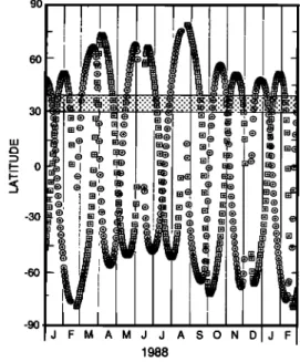
9O 6O 3O -3O -6O -9O O F M A M O O A S O N D 1988 j F
Fig. 1. SAGE II orbit and measurement locations during 1988. The circles indicate an occultation measurement at sunrise and the
squares, a measurement at sunset. Measurements made within the
shaded area were used in the zonal mean comparisons.
photon-counting system. At this point a second channel was added for each wavelength, to receive ---10% of the returned signal and thus effectively increase the dynamic range by one decade; these channels allowed an ozone profile measure- ment between 20 km and 40 km. Each wavelength pair, simply referred to as high channels and low channels, is analyzed independently. Thus two profiles are produced which overlap between 30 km and 40 km. The two profiles normally agree within 1 or 2% in this region, and agreement within the error bars is always expected. If the profiles do not agree well, this is an indication of some problem, and experience has shown that this is most likely due to the background level calculation which can be adversely af- fected by misalignment of the transmitter-receiver and to the effects of a bright moon close to zenith. A composite profile is made up using the low-channel data from 20 km to ---30 km and the high channel data from ---30 km to 50 km.
The SAGE II (Stratospheric Aerosol and Gas Experiment) instrument is a seven-channel, limb-scanning sun photome- ter using the solar occultation technique, and was launched onboard the Earth Radiation Budget Satellite (ERBS) in
October 1984. Ozone concentrations are inferred from the
0.6/am radiances with a precision of ---5% between 24 and 36 km, degrading to 7% at 48 km, for a vertical correlation distance of 3 km. The latitude range extensively sampled is 65øS to 65øN with a roughly 1 month repeat cycle. The measurements at a particular latitude are grouped over several days, as can be seen in Figure 1 where the shaded band indicates the 34.4 ø _ 5 ø zone of interest. The concept of a monthly mean is not appropriate for such grouping, and instead the approach used is to average the group of mea- surements about the mean day.
The altitude-range resolution and the typical experimental
uncertainties are different for the lidar and the SAGE II
instruments. For the lidar, the altitude resolution is a fixed function and is ---1 km up to 30 km, increasing to 3 km at 40
MCDERMID ET AL.' LIDAR-SAGE II STRATOSPHERIC OZONE COMPARISON 5607
TABLE 1. Dates of Ozone Profile Measurements
Jan. Feb. March April May June July Aug. Sept. Oct. Nov. Dec.
6 HL 7 8 9 HL 10 HL 11 HL 12 HL 13 HL 14 15 16 HL 17 HL 18 HL 19 HL 20 21 22 23 24 25 HL 26 HL 27 HL 28 29 30 HL 31 H H H H H H H HL HL HL H H H HL HL H H HL HL HL H HL HL H HL HL HL HL HL HL H HL HL H H HL H HL HL H HL HL H H HL HL H HL H H HL HL HL HL HL HL H H H HL HL HL HL H H H HL H HL H HL HL H HL H HL HL HL H H HL H HL H HL H H HL HL HL HL H HL HL HL HL
The date refers to the evening that the experiment began, even if it continued past midnight. H and L indicate whether data are available from the high channels (30 km to 50 km) and low channels (20 km to 40 km), respectively. Because of the limited number of experiments in January 1988, and also the fact that only high channel data were available at that time, the results from January 1989 have been used in
this paper and are indicated in this table.
km and to 7.5 km at 50 km. The uncertainty, statistical error, is dependent on a number of factors. The most important of these are the clarity of the atmosphere, particularly the troposphere, and the output power of the laser system. Since both of these factors vary from day to day, there is not a typical single value for the statistical error, but there is a normal range. Up to 35 km altitude the error is -< 1% and increases to 2-4% at 40 km. At 45 km and above, the uncertainties in the lidar measurement increase rapidly from ---3-10% at 45 km to 10-25% at 50 km. Also, at these altitudes the calculated ozone concentration is very sensitive to the background level, and significant biases, toward higher ozone values, have been observed in measurements taken on nights when the moon was bright and close to zenith. Some of these points can be seen in the 50 km plot of Figure 3. This problem only occurs at the highest altitudes, above 45 km, and does not affect the profile at lower altitudes. For the purposes of this comparison no data points have been omitted from the record even though it would be justified to omit the points at 50 km, and to some extent 45 km, that were obtained under conditions of high background moonlight.
RESULTS
During the year, from February 1988 through January 1989, 111 ozone concentration profiles were recorded be- tween 30 km and 50 km and of these, 68 measurements also
included ozone profiles down to 20 km altitude. The dates of the ozone profile measurements made by the lidar instru- ment are shown in Table 1. Owing to the uneven distribution of these measurements through the year, some caution must be used when considering yearly means as these will be biased to those months with the greater numbers of mea- surements, which for this data set are the months October to January.
The lidar data were first compared with two ozone refer- ence models, the Krueger and Minzner [1976] mid-latitude ozone model for the U.S. Standard Atmosphere (1976) and the Keating and Pitts [1987], Keating et al. [1987] reference model for CIRA. The results are shown in Figure 2. The individual lidar data points were averaged on a monthly basis and are shown by the solid lines in Figure 2. The 1 cr standard deviation of these measurements is indicated by the shaded areas. The Krueger and Minzner [1976] model provides an
estimate of the mean annual ozone concentration for an
effective latitude of 45øN. No attempt has been made to adjust this model to 34øN, and the ozone values are shown by the dotted lines in Figure 2. The Keating and Pitts [1987], Keating et al. [1987] model gives monthly zonal mean ozone concentrations for 10 ø latitude increments, and these data have been interpolated to provide values corresponding to 34øN and are shown by the dashed line in Figure 2.
The lidar results were next compared with measurements made by the SAGE II. For these comparisons, only SAGE II
5608 MCDERMID ET AL.' LIDAR-SAGE II STRATOSPHERIC OZONE COMPARISON 5.0E+ 12 I E
• 4.5E+12
z '•: 4.0E+12 Z Z O N O 3.5E+ 12 i ß a i i i i i i i i i 0 30 60 90 120 150 180 210 240 270 300 330 360 390 DAY NUMBER 3.5E+ 12 I E o • 3.0E+ 12 z c:3 2.5E+12 m z 2.0E+12 Z O N O 1.5E+12 0 30 120 150 180 210 24.0 270 300 330 360 390 DAY NUMBER1.8E
+
12
[
'••.
r/T::',
•
•..:.:.:.:.:i!iii•
-
...{?:'.
::::::::::::::::::::::: 1.4.E+ 12 ... ß :.:.:-: ---"l O '=• 1.6E+1 2 1.0E+12 i ß • i i i i i i i i i 0 30 60 90 120 150 180 210 24-0 270 300 330 360 390 DAY NUMBER 8.0E+11 I E o '=• 7.0E+ 11 z c:3 6.0E+ 11 m z 5.0E+11 Z O N O 4.0E+11 i ß . i i . i i i i i i 0 30 60 90 120 150 180 210 24-0 270 300 330 360 390 DAY NUMBER 3.5E+11 I E o• 2.5E+11
z m '•: 1.5E+11 Z Z O N O 5.0E+ 10 ... 0 30 60 90 120 150 180 210 240 270 300 330 360 390 DAY NUMBER 3.0E+ 11 I E o• 2.0E+
11
z,•1.0E+
11
Z Z O N O 0.0E+0050
krn
]
...
:::...
"..-iiii...ii::::ii::::!::i
0 30 60 90 120 150 180 210 240 270 300 330 360 390 DAY NUMBERFig. 2. Comparison of the lidar monthly means, indicated by the solid line and with 1 cr standard deviation indicated by the shaded area, compared with the monthly values at 34øN from the CIRA reference atmosphere, shown by the dashed line, and compared with the U.S. Standard Atmosphere (1976), represented by the dotted line.
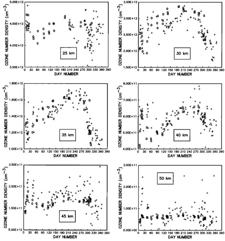
measurements made within a radius of 1000 km from the
lidar site were considered. For the same period as the lidar experiments, February 1988 to January 1989, there were 36 SAGE II measurements that met this criterion. However, none of the measurements were at precisely the same location and, since the SAGE II is a sun-observing instru- ment and the lidar operates only at night, the measurements
are never made at the same time. The mean location of the 36
SAGE II measurements considered was +35.0øN, -116.9øW, compared to the lidar location at +34.4øN,
-117.7øW, and the mean distance between the measure- ments was 715 km. The individual data points are shown in Figure 3 where the open circles are the SAGE II measure-
ments and the crosses are the lidar measurements.
The closest measurements were made on October 31,
1988, when the SAGE II made a sunrise measurement at 34.48øN, -114.94øW, which is 240 km essentially directly
east of the lidar. For this SAGE II sunrise measurement
there were lidar measurements made during both the night before and the night after, and therefore these data provide
MCDERMID ET AL.' LIDAR-SAGE II STRATOSPHERIC OZONE COMPARISON 5609 5.00E+ 12 I E o
• 4,50E+12
z ß • 4,00E+12 Z Z O N O 3,50E+ 12 o o oo • ø
o25
krn
I
+ + ++.o.•t++
•'•+
+
+
+++ +
+ + + i i i i i i i i i -t-, i i 0 30 60 90 120 150 180210240270300330360390 DAY NUMBER 3.50E+ 12 I E o "-" 3,00E+12 z • 2,50E+12 Z 2.00E+12 Z O N O 1,50E+ 12 4• +++
o •
++0 .0
•0 +
++
+
+ •0 0 0++•
•+ ++ 0 +• + • + + +•I
+ 0 + +0 + +•o
++ + +"
o+
o
I I :+
30 krn
. i i i . i i i i . . , 0 30 60 90 120 150 180210240270300330360390 DAY NUMBER 1,80E+ 12 • 1.60E+12 Z • 1.40E+12Z• 1.20E+12
Z O N O 1.00E+ 12 -i- -i-+++
o+,
0+• + 0 ++
+ + /•-0
++
•0 '0•+
++*
+t
+% +•+
++++•
+
+
{)++-'t
õ o +35
krn[
ß .14-+ +++
0 30 60 90 120 150 180210240270300330360390 DAY NUMBER 8.00E+ 11 I E o • 7.OOE+11 z • 6.00E+11 Z 5.00E-I-11 Z O N O 4.00E+11 + + + -i-, +
+
6 +
+ + +•)
•.
0 + ++
+oat++
+ + o o++.o
+
• + 40
krn
og
0 30 60 90 120 1,50 180210240270300330360390 DAY NUMBER • + + + -N-++•. +•- +
+ ++#
+ 3.50E+ 11 I E o• 2.50E+11
i z ß • 1.50E+11 + + + + + ++ +* +
% +
+ + ++ + + + + + +0 +
-•'+'
0 o+++
•++ + Z + + ++ Z O N ++ o . . . , , õ.00E+ 10 ' ' ' ' ' , 0 ,.NO 60 90 120 1,50 180 210 24-0 270 300 330 360 390 DAY NUMBER 3.00E+ 11 I E o• 2,00E+11
z ß • 1.00E+11 Z Z O N O 0,00E+00 + + + + + +•.+ •
+ +++
++ + ++
+ ++•+
+
+
+
+•++
+•+•+
' I I + I I I I I I I + I 0 30 60 90 120 150 180 210 240 270 300 330 360 390 DAY NUMBERFig. 3. Comparison of individual lidar measurements (crosses) and individual SAGE II measurements made within 1000 km of the lidar (circles).
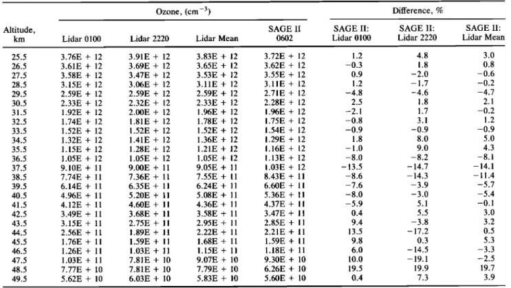
the best opportunity for a detailed one-to-one comparison. To enable direct comparison, the lidar data were interpo- lated, using a cubic spline routine, to obtain ozone concen- trations at the same altitudes as the SAGE II profile. The three profiles, two lidar and one SAGE II are shown in Figure 4. The logarithmic and linear scales are used to show the differences more clearly at high and low altitudes, respectively. Table 2 compares these profiles quantitatively, and it can be seen that for most of the range the agreement is better than 5%. However, there are some features which can be seen in the profiles in Figure 4 where the difference is
greater, reaching a maximum of-19%. It should be noted that this comparison represents one of the best cases. Even for measurements within 1000 km of each other the profiles sometimes show significant differences which have been assumed to be due to the different location, primarily lati- tude, and different airmasses.
Finally, the lidar data were compared with the zonal mean
of the SAGE II measurements within the band 34.4 ø _+ 5øN.
For each mean day, up to 36 individual SAGE II measure- ments were averaged. Figure 5 shows these means, and their standard deviations, overlaid on the lidar monthly means.
5610 MCDERMID ET AL.' LIDAR-SAGE II STRATOSPHERIC OZONE COMPARISON 25 1.00E+ 10 -- LIDAR -- 01:00 . o SAGE II 06:02 __ -. LIDAR .... 22:20 5O -- LIDAR ' ' 01:00 o SAGE II 06:02 ... LIDAR 22:20
,
251.00g+11 1.00E+12 1.00g+13 O.00g+00 1.00g+12 2.00E+12 3.00g+12 4.00g+12
OZONE
NUMBER
DENSITY
(cm
-3)
OZONE
NUMBER
DENSITY
(cm
-3)
Fig. 4. Comparison of SAGE II and lidar ozone profiles measured on October 31, 1988. These represent the measurements closest in both time and location for the entire year. The times (PDT) of the measurements are indicated on the plots. The quantitative differences between these profiles are given in Table 2.DISCUSSION
The overall agreement between the lidar and SAGE II data sets, and the CIRA ozone reference model is very good. As is to be expected, the best agreement is found between the
individual lidar measurements and SAGE II measurements
made within 1000 km of JPL TMF, although the agreement between the lidar and the SAGE II zonal means is also very good for 30 km and higher altitudes as also might be anticipated because of the inherent greater variability in ozone below 30 km where dynamics dominate photochem- istry. Also, one-to-one comparisons show agreement to
better than 5% over most of the range when the measure- ments were almost simultaneous in time and space.
An attempt to quantify the overall agreement between the SAGE II and lidar measurements has been made by calcu- lating a yearly average ozone concentration for each altitude
and instrument. For SAGE II the 36 measurements made
within 1000 km of the lidar were simply averaged. For the lidar the monthly means were averaged instead of the individual points in an attempt to eliminate some of the biases caused by different numbers of measurements in each month. The results are shown in Table 3. At 45 and 50 km,
TABLE 2. Comparison of SAGE II and Lidar Ozone Profiles Measured on October 31, 1988
Ozone, (cm -3) Difference, %
Altitude, SAGE II SAGE II' SAGE II: SAGE II'
km Lidar 0100 Lidar 2220 Lidar Mean 0602 Lidar 0100 Lidar 2220 Lidar Mean
25.5 3.76E + 12 3.91E + 12 3.83E + 12 3.72E + 12 1.2 4.8 3.0
26.5 3.61E + 12 3.69E + 12 3.65E + 12 3.62E + 12 -0.3 1.8 0.8
27.5 3.58E + 12 3.47E + 12 3.53E + 12 3.55E + 12 0.9 -2.0 -0.6
28.5 3.15E + 12 3.06E + 12 3.11E + 12 3.11E + 12 1.2 -1.7 -0.2
29.5 2.59E + 12 2.59E + 12 2.59E + 12 2.71E + 12 -4.8 -4.6 -4.7
30.5 2.33E + 12 2.32E + 12 2.33E + 12 2.28E + 12 2.5 1.8 2.1
31.5 1.92E + 12 2.00E + 12 1.96E + 12 1.96E + 12 -2.1 1.7 -0.2
32.5 1.74E + 12 1.81E + 12 1.78E + 12 1.75E + 12 -0.8 3.1 1.2
33.5 1.52E + 12 1.52E + 12 1.52E + 12 1.54E + 12 -0.9 -0.9 -0.9
34.5 1.32E + 12 1.41E + 12 1.36E + 12 1.29E + 12 1.8 8.0 5.0
35.5 1.15E + 12 1.28E + 12 1.21E + 12 1.16E + 12 -1.0 9.0 4.3
36.5 1.05E + 12 1.05E + 12 1.05E + 12 1.13E + 12 -8.0 -8.2 -8.1
37.5 9.10E + 11 9.00E + 11 9.05E + 11 1.03E + 12 -13.5 -14.7 -14.1
38.5 7.74E + 11 7.36E + 11 7.55E + 11 8.43E + 11 -8.6 -14.3 -11.4
39.5 6.14E + 11 6.35E + 11 6.24E + 11 6.60E + 11 -7.6 -3.9 -5.7
40.5 4.96E + 11 5.20E + 11 5.08E + 11 5.36E + 11 -8.0 -3.0 -5.4
41.5 4.12E + 11 4.60E + 11 4.36E + 11 4.37E + 11 -5.9 5.1 -0.1
42.5 3.49E + 11 3.68E + 11 3.58E + 11 3.47E + 11 0.4 5.5 3.0
43.5 3.15E + 11 2.75E + 11 2.95E + 11 2.85E + 11 9.4 -3.8 3.2
44.5 2.56E + 11 1.89E + 11 2.22E + 11 2.21E + 11 13.5 - 17.2 0.5
45.5 1.76E + 11 1.59E + 11 1.68E + 11 1.59E + 11 9.8 0.3 5.3
46.5 1.26E + 11 1.03E + 11 1.15E + 11 1.18E + 11 6.0 -14.5 -3.3
47.5 1.03E + 11 7.81E + 10 9.07E + 10 9.30E + 10 10.0 -19.1 -2.5
48.5 7.77E + 10 7.81E + 10 7.79E + 10 6.26E + 10 19.5 19.9 19.7
49.5 5.62E + 10 6.03E + 10 5.83E + 10 5.60E + 10 0.4 7.3 3.9
MCDERMID ET AL.' LIDAR--SAGE II STRATOSPHERIC OZONE COMPARISON 5611 5.0E+ 12
1
E
_ 4,5E+12•,• 4.0E+12
Z Li.I Z O N O 'r 3.5E+12 0 30 60 90 120 150 180 210 24.0 270 300 330 360 390 DAY NUMBER 3.5E+ 12 1 E o '-' 3.0E+ 12 z t:3 2,5E+12 Z 2.0E+12 Z O N O 1.5E+1 2iO I ; I I . i i i i . i
0 60 9 120 150 180 210 24-0 270 300 330 360 390 DAY NUMBER 1.8E+1 2 "' 1.6E+12 Z e,• 1.4E+ 12 Z 1.2E+ 12 Z O N O35
km
I
1.0E+12 ... ' • ' ' ' ' ' 0 30 60 90 120 150 180 210 240 270 300 330 360 390 DAY NUMBER 8,0E+11 I E o '-' 7.0E+11 z • 6,0E+11 Z 5.0E+11 Z O N O 4.0E+ 11I dO I I I I I I i . I I
•0 90 120 160 180 210 240 270 •00 •0 •60 •90 DAY NUMBER 3.5E+ 11• 2.5E+11
Z '•: 1,5E+ 11 Z Z O N O 5.0E+ 10 ... 0 30 60 90 120 150 180 210 24.0 270 300 330 360 390 DAY NUMBER 3.0E+11• 2.0E+11
Z•'• 1.0E+11
Z Z O N O 0.0E+005o
km
I
...
II I ;0 i I i
0 30 60 120 150 180 210 24-0 270 300 330 360 390 DAY NUMBERFig. 5. SAGE II zonal mean values and 1 rr standard deviation (circles and error bars) overlaid on the lidar monthly
means and 1 rr standard deviation (solid line and shaded area).
some of the difference may be attributable to some of the lidar data having too high ozone values due to biases caused by moonlight (all data were considered in forming the averages). Also, there were no SAGE II measurements within 1000 km during June, August, and December. For all of the altitudes, June and August tend to be months with higher ozone concentrations, and their omission would tend to reduce the SAGE II yearly average.
The annual (AO) and semiannual (SAO) oscillatory behav- ior in the ozone concentration profile is clearly shown in Figures 3 and 4. Such time-periodic variations, as observed
by SAGE II, have been described in detail by Wang et al. [1988] for the latitude bands -45 ø to -35 ø , -5 ø to 5 ø , and 35 ø to 45 ø. Here, for 34.4øN, we find a single AO peaking in July for 30 km and 35 km, similar to that observed by Wang et al. [1988] for 40øN. The peak-to-peak magnitude of this oscilla- tion is greatest at 30 km and is of the order of 0.8 to 1.0 x
1012
molecule
cm -3. At 40, 45, and 50 km there is a double
oscillation, SAO, with one maximum in February for all and with a second maximum, in September at 40 km, a broad peak from July to September at 45 km, and in July at 50 km.
5612 MCDERMID ET AL.' LIDAR-SAGE II STRATOSPHERIC OZONE COMPARISON
TABLE 3. Comparison of SAGE II and Lidar Yearly Average Ozone Concentration for Various Altitudes
Lidar Yearly SAGE II
Mean Yearly Mean
Altitude, Ozone, Ozone, Difference Lidar ß
km cm -3 cm -3 SAGE II, % 30 2.73E + 12 2.77E + 12 -1.5 35 1.43E + 12 1.40E + 12 2.1 40 6.02E + 11 5.65E + 11 6.1 45 2.05E + 11 1.79E + 11 12.7 50 6.85E + 10 5.95E + 10 13.1 Read 2.73E + 12 as 2.73 x 10¹²
1984 to 1987 by SAGE II at 40øN and is qualitatively more similar to the SAO observed at 0 ø and 40øS, although the phase is different. At 25 km the lidar data are limited, but the
SAGE II data show a SAO with maxima in December-
January and June-July. This agrees, in terms of phase and period, with the previous SAGE II observations; however, the amplitude of the July peak is greater. Since this data set is limited to only a single annual cycle, some caution must be exercised not to overinterpret the conclusions.
We believe that this study confirms the power of the lidai technique for making accurate measurements of strato- spheric ozone profiles. These comparisons should continue
as a check on both sensors and as a validation in the
determination of long term trends. It also demonstrates the ability to make correlative measurements with satellite in- struments such as SAGE II, and also the future generation of
instruments that will be carried onboard the UARS and EOS
space platforms.
Acknowledgments. The work described in this paper was car- ried out at the Jet Propulsion Laboratory, California Institute of Technology, and at the Langley Research Center (LaRC) under contracts with the National Aeronautics and Space Administration. We are grateful for the assistance of Daniel Walsh, Oscar Lindqvist,
and David Haner in the setup and operation of this lidar system and to G. M. Keating of NASA LaRC for providing us with a tape of the new COSPAR (CIRA) ozone reference model. We would also like to thank the National Research Council for the award of an associate- ship to S.M.G.
REFERENCES
Cunnold, D. M., W. P. Chu, R. A. Barnes, M.P. McCormick, R. E. Veiga, and D. A. Chu, Error analysis and validation of SAGE II ozone measurements, in Proceedings of the Quadrennial Ozone Symposium, edited by R. D. Bojkov and P. Fabian, p. 145, A. Deepak, Hampton, Va., 1988.
Cunnold, D. M., W. P. Chu, R. A. Barnes, M.P. McCormick, and R. E. Veiga, Validation of SAGE II ozone measurements, J Geophys. Res., 94, 8447-8460, 1989.
Keating, G. M,, and M. C. Pitts, Proposed reference models for ozone, Adv. Space Res., 7, 37-47, 1987.
Keating, G. M., D. F. Young, and M. C. Pitts, Ozone reference models for CIRA, Adv. Space Res., 7, 105-115, 1987.
Krueger, A. J., and R. A. Minzner, A mid-latitude ozone model for the 1976 U.S. Standard Atmosphere, J. Geophys. Res., 81,
4477-4481, 1976.
McDermid, I. S., Ground-based lidar and atmospheric studies, Surv. Geophys. 9, 107-122, 1987.
Wang, P.-H., M.P. McCormick, L. R. McMaster, S. Schaffner, and G. E. Woodbury, Time-periodic variations in stratospheric ozone from satellite observations, in Proceedings of the Quadrennial Ozone Symposium, edited by R. D. Bojkov and P. Fabian, p. 143, A. Deepak, Hampton, Va., 1988.
World Meteorological Organization, Report of the International Ozone Trends Panel--1988, Rep. 18, Geneva, in press, 1989. S. M. Godin, Service d'Aeronomie du CNRS, Universit6 Paris
VI, 4 Place 75230 Paris Cedex 05, France.
M.P. McCormick, Aerosol Research Branch, Atmospheric Sci- ences Division, NASA Langley Research Center, Hampton, VA 23665.
I. S. McDermid, Table Mountain Facility, Jet Propulsion Labo- ratory, California Institute of Technology, Wrightwood, CA 92397. P.-H. Wang, Science and Technology Corporation, 101 Research Drive, Hampton, VA 23666.
(Received July 24, 1989'
revised September 5, 1989' accepted September 6, 1989.)