Ali
Kazerani
B.A.Sc., University of Waterloo (2010)
Submitted to the Department of Electrical Engineering and Computer
Science
in partial fulfillment of the requirements for the degree of
Master of Science in Electrical Engineering and Computer Science
at the
MASSACHUSETTS INSTITUTE OF TECHNOLOGY
June 2013
©
Massachusetts Institute of Technology 2013. All rights reserved.
A u th or ... . ....
...
Department of Electrical Engineering and Computer Science
May 22, 2013
C ertified by ...
...
ICertified by....L...
...
John N. Tsitsiklis
Professor
Thesis Supervisor
...
George C. Verghese
Professor
Thesis Supervisor
Accepted by.
/6/0
Leslie A. Kolodziejski
Chairman, Departmental Committee on Graduate Students
Ali Kazerani
Submitted to the Department of Electrical Engineering and Computer Science on May 23, 2013, in partial fulfillment of the
requirements for the degree of
Master of Science in Electrical Engineering and Computer Science
Abstract
In this thesis, we develop and analyze a simple grey-box model that describes the pathophysiology of central sleep apnea (CSA). We construct our model following a thorough survey of published approaches. Special attention is given to PNEUMA, a complex, comprehensive model of human respiratory and cardiovascular physiology that brings together many existing physiological models. We perform a sensitivity analysis, concluding that signals of interest in PNEUMA are insensitive to changes in all but approximately twenty parameters. This justifies our goal of developing a small, simple model that captures approximately the same behaviour among signals of interest. The simplicity of our model not only makes it accessible to analytical and intuitive exploration, but also opens up the possibility that its parameters could be reliably estimated from a patient's data records. This could be of great value in developing patient-specific or state-specific treatments for CSA.
Our model describes the dynamics of the alveolar gas exchange, blood gas transport, and cerebral gas exchange processes, which together determine the cerebral and arterial partial pressures of carbon dioxide, given ventilation as input. Our model of the ventilatory controller senses both the cerebral and arterial carbon dioxide partial pressures and issues a ventilatory drive command from which the level of ventilation is determined, closing the loop. We develop a linearized small-signal model of our system and determine conditions for its stability. We conclude by comparing the stability predictions suggested by our linear analysis to the stability properties of our original nonlinear model, with promising results.
Thesis Supervisor: John N. Tsitsiklis Title: Professor
Thesis Supervisor: George C. Verghese Title: Professor
fortunate to work with you. Thank you for demonstrating, without fail, every professional and personal virtue imaginable, along with something resembling omniscience. And of course, thank you in particular for all the guidance you offered as I wrote (and you read) this thesis.
Thanks also to Dr. Thomas Heldt, who taught me so much both in class and during research meetings.
I would like to thank the Periodic Breathing Foundation for a generous gift to MIT, which made this work possible. I offer my sincere thanks also to Robert Daly, for the inspiration he provided and for sharing his experience and expertise with us in discussions, meetings, and tours.
I am incredibly grateful to all those who guided and helped me while, not so very long ago, I was searching for a research home. My thanks in particular to Professors Leslie Kolodziejski and Alan Oppenheim, for looking after me through the tumult. I would also like to thank Janet Fischer for all her help and apparently inexhaustible patience. And I will forever owe a great debt to Professor Terry Orlando, who spent a great many hours over many months helping me find and make my way in this place. My journey would have been very, very different if I had not met him.
PNEUMA, a physiological model implementation that I explore in this thesis, is supported and distributed by the University of Southern California Biomedical Simulations Resource.
1 Introduction 13
1.1 Background . . . . 13
1.2 Literature Survey . . . . 15
1.3 Contributions and Outline . . . . 17
2 PNEUMA 21 2.1 Introduction to PNEUMA . . . . 21
2.2 Simulating Stable and Unstable Breathing in PNEUMA . . . . 23
2.3 Issues with PNEUMA . . . . 26
2.4 Preparing PNEUMA for Numerical Experiments . . . . 29
2.5 Sensitivity Analysis . . . . 30
2.5.1 Our Procedure . . . . 31
2.5.2 Some Additional Details . . . . 34
2.5.3 R esults . . . . 36
2.5.4 Conclusions . . . . 41
3 A New, Simple Model 43 3.1 Overview . . . . 43
3.1.1 Pulmonary Gas Exchange Plant, PA . . . . 44
3.1.2 Lung-to-Carotid Transport Plant, Pa . . . .. 45
3.1.3 Cerebral Gas Exchange Plant, Pb . . . . 46
3.1.4 Chemoreflex Controller . . . . 47
3.1.5 Ventilation Plant . . . . 47 7
3.2 Model Properties ... 48
3.2.1 Requirements . . . . 48
3.2.2 Simplifications . . . . 48
3.3 Model Details . . . . 49
3.3.1 Pulmonary Gas Exchange Model . . . . 49
3.3.1.1 Linearization . . . . 53
3.3.2 Cerebral Gas Exchange Model . . . . 55
3.3.3 Lung-to-Carotid Transport Model . . . . 61
3.3.4 Chemoreflex Control of Ventilation . . . . 74
3.4 Model Parameters . . . . 85
3.4.1 The System Operating Point . . . . 89
3.5 Simulation Results . . . . 93
3.5.1 Incorporating Pad6 Approximants . . . . 94
3.5.2 Using Linearized Plant Models . . . . 96
4 Stability Analysis 101 4.1 Linear Stability Analysis . . . 101
4.1.1 The Linearized Model . . . 101
4.1.2 Stability of the Linear Model System . . . 104
4.2 Influence of Central and Peripheral Gains on Stability . . . 111
4.3 Stability of our Nonlinear Model System . . . 116
5 Conclusion 121 5.1 Future Work . . . .. . . . 122
1.1 Lung volume waveforms for normal breathing and CSA. . . . . 15
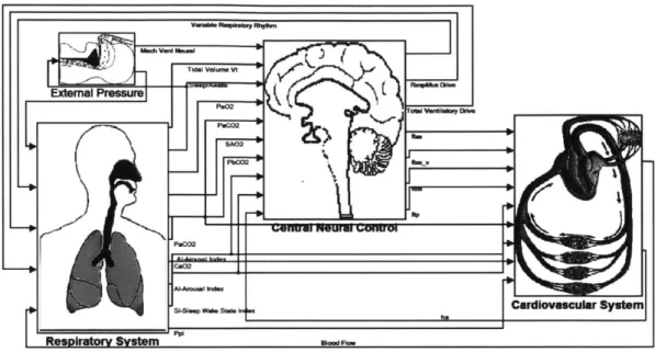
2.1 PNEUMA's top-level block diagram. . . . . 23
2.2 PNEUMA-simulated waveforms representing normal, steady conditions in sleep. . . . 24
2.3 PNEUMA-simulated waveforms representing CSA. . . . . 25
2.4 The continuous tidal volume and arterial carbon dioxide tension waveforms. . . . . . 31
2.5 J and i. ... ... ... . ... 33
2.6 Sensitivity versus parameter rank, for v' . ... . 36
2.7 Sensitivity versus parameter rank, for &. . . . . 37
2.8 Sensitivity versus parameter rank, for T. . . . . 37
2.9 Baseline and perturbed -i3 waveforms for the six highest-ranked parameters. ... 39
2.10 Baseline and perturbed - waveforms for the six highest-ranked parameters. . . . . . 40
3.1 Block diagram of our new, simple model. . . . . 44
3.2 Autoregulation of cerebral blood flow. . . . . 57
3.3 Step response of Lange model. . . . . 65
3.4 Step responses of D1M and DOM models best fitting the D2M step response . . . . . 67
3.5 Responses of D2M, D1M, and DOM models to sinusoidal input. . . . . 69
3.6 Responses of Pad6-approximated transport models to sinusoidal input. . . . . 71
3.7 Phase delay versus period, for adjusted and unadjusted Pade-approximated transport m od els. . . . . 73
3.8 Filtered Pa,C02 and Sa,0 2 waveforms from PNEUMA simulation of CSA. . . . . 79
3.9 [jPa,CO2 - Pa,C02,TH]+, [SaO2,TH - Sa,02]+, and [Pa,CO2 - Pa,CO2,TH]+ [Sa,02,TH - Sa,0 2]±
w aveform s. . . . 80 3.10 GPNEU.M A,a jPa,C0 2 - Pa,C02,TH]+ [Sa,02,TH - Sa,021+ and Ga jPa,C02 - Pa,C02,TH]+
w aveform s. . . . 80 3.11 Ventilation, tidal volume, and respiratory rate versus chemical drive, in PNEUMA. . 82 3.12 The subsystem made up of the gas exchange and transport model systems. . . . . 91 3.13 Steady-state CSA simulation results from our model (black) and PNEUMA (red). . 94 3.14 Simulation results from our model when Pad6-approximated transport models are used. 95 3.15 Simulation results from our model when linearized gas exchange models are used. . . 96 4.1 Our large-signal linearized model. . . . . 4.2 Our small-signal linearized model .. . . . . 4.3 The
XA=
0 hyperbola in the first quadrant of the (G', G') plane. . . . . 4.4 Stable and unstable regions in the (G', G') plane. . . . . 4.5 Stability boundary, along with numerically-determined stability of points in the(G' ,G') plane, using m = n = . . . . 4.6 Stability boundary using m= n = 1, along with numerically-determined stability of
points in the (G', G') plane, using m = n = 2 and m = n = 3. . . . . 4.7 Stability of the nonlinear and linearized models. . . . .
103 103 115 116 117 118 119
Parameter values for our pulmonary gas exchange plant (PA) model. Parameter values for our lung-to-carotid transport plant (Pa) model. Parameter values for our cerebral gas exchange plant (Pb) model. . . Parameter values for our chemoreflex controller model. . . . . Parameter values for our ventilation plant model. . . . . Equilibrium operating points for our model. . . . .
The Routh array. . . . . Four possible sign sequences for the second column of the Routh array. Characteristics of zeros implied by signs of Routh array elements. . . .
. . . . 85 . . . . 86 . . . . 87 . . . . 88 . . . . 89 . . . . 93 . . . 106 . . . . 107 . . . 109 11 3.1 3.2 3.3 3.4 3.5 3.6 4.1 4.2 4.3
Introduction
In this thesis, we develop and simulate a simple grey-box physiological model of central sleep apnea, following a review of existing models. We then develop a linear approximation of the behaviour of our model system in the vicinity of its equilibrium operating point, and describe the regimes in which this linear system is stable. Finally, we compare the predictions of our linear stability analysis to the behaviour of the original model.
We begin with an introduction to the pathophysiology of central sleep apnea.
1.1
Background
In a normal, healthy individual, respiration is under tight control, ensuring that oxygen (02) is brought into the body at a rate that meets tissue demand, and carbon dioxide (C0 2) is expelled at
a rate matching that of CO2 production by the tissues. The dominant mechanism of control is the
respiratory chemoreflex: chemosensors detect the levels of 02 and CO2 in the oxygenated blood
leaving the lungs and direct adjustments in ventilation that tend to normalize blood gas levels. For instance, if the level of carbon dioxide in the blood is elevated (depressed), the chemoreflex directs an increase (decrease) in ventilation to return the blood CO2 level to some setpoint.
Ventilation determines the rate at which fresh air enters the alveoli (the gas exchange regions of the lungs). Oxygen and carbon dioxide are exchanged between the air in the alveoli and the blood in the pulmonary capillaries that perfuse them. Ventilation therefore directly influences the
'We use the terms "chemosensor" and "chemoreceptor" interchangeably.
gas content of the pulmonary capillary blood leaving the alveoli. The chemosensors, however, are not situated in the lungs, so they do not measure the levels of gases in the alveolar air or the pulmonary end-capillary blood (with which the alveolar air is in equilibrium). Let PA denote the partial pressure2 of carbon dioxide in the alveolar air and pulmonary end-capillary blood.
Once blood from the pulmonary capillaries merges in the pulmonary vein, it enters the heart, is pumped out into the aorta, and there encounters the first set of peripheral (arterial) chemosensors: the aortic chemosensors. Further downstream, the blood encounters the carotid chemosensors, which make up the second set of peripheral (arterial) chemosensors. Even further along, CO2 in the arterial
blood influences the pH of cerebrospinal fluid, which is detected by the central chemoreceptors in the brainstem. Each cluster of chemosensors therefore detects a version of PA delayed by a length of time determined by its location and by the rate of blood flow. Furthermore, even correcting for delays, the time course of PA differs from the time course of CO2 tension at each set of chemoreceptors,
since the blood in which the gas is transported undergoes mixing, and the central chemoreceptors do
not directly measure the carbon dioxide content of the blood. Finally, the contribution of each set
of chemoreceptors to the overall ventilatory drive exhibits its own characteristic gain and dynamics.
In some individuals, irregularities in the chemoreflex (such as prolonged transport delay and elevated chemoreflex gain) render the closed-loop system unstable, resulting in oscillations in
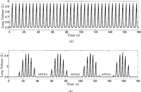
venti-latory drive. If the oscillations are sufficiently severe, ventilation is sometimes excessive (hyperpnea), sometimes present but insufficient to remove carbon dioxide from the blood at an appropriate rate (hypopnea), and sometimes completely absent (apnea). Figure 1.1 shows ventilation patterns in computer-simulated cases of stable and unstable breathing. The closed-loop system is especially vulnerable during sleep, leading in extreme cases to central sleep apnea (CSA), a disorder whose sufferers experience frequent apneas in their sleep. These periods of zero ventilation are associ-ated with a number of acute disruptions (such as arousals and cardiovascular shocks) and chronic health problems (such as chronic hypertension). One particularly regular form of unstable breathing caused by chemoreflex instability is Cheyne-Stokes respiration (CSR), which is especially prevalent in individuals suffering from congestive heart failure (CHF).
2
2.7- bO2.6-2.5 0 20 40 60 80 100 120 140 160 180 Time (s) (a) 3.5-
3--APNEA APNEA APNEA
0 20 40 60 80 100 120 140 160 180
Time (s)
(b)
Figure 1.1: Computer-simulated lung volume waveforms in (a) stable and (b) unstable breath-ing caused by prolonged blood transport delay and elevated chemoreflex gain. Simulations were performed in Simulink, using the PNEUMA model described in [CIFK1O].
1.2
Literature Survey
A Simple Toy ModelVery simple models have been proposed that, when simulated, generate periodic ventilation patterns similar to those that are characteristic of CSR. The earliest of these is the model of Mackey and Glass, which consists of a single equation in which the rate of carbon dioxide buildup in the blood is determined by ventilation - the volume flow rate of air into (or out of) the lungs, averaged over each inspiration (expiration) [KS09]. To model the chemoreflex, ventilation is described as a sigmoidal function of the delayed alveolar carbon dioxide partial pressure. A stability analysis shows that sufficiently high chemoreflex gains and transport delays will lead to instability. With parameters
thus selected, time domain simulations show oscillatory ventilation and carbon dioxide tension.
While the model's simplicity makes it accessible to analysis and intuitive understanding, it is rather removed from real physiology, and we would not expect it to be able to capture very many patterns relevant to treatment or diagnosis, nor would we expect it to reproduce real ventilation waveforms
with any fidelity.
A Complex Model
Near the opposite end of the spectrum is the early and very complex model of Grodins et al. [GBB67]. It describes, amongst other things, the dynamics of oxygen, carbon dioxide, and nitrogen levels in the compartments representing the lungs, the brain, and the remaining body tissues. Air flows into and out of the lung compartment, and blood carries gases from the lungs to the brain and tissues, then back to the lungs. Ventilation is determined in response to both peripheral and central cues, and cardiac output is changed in response to changes in arterial gas levels. Cardiac output-dependent delays represent the time needed for blood to carry gases between pairs of compartments. The model equations are numerous and complex, and there are many state variables and parameters.
Intermediate-Complexity Models
The significantly more tame model of Khoo et al. [KKSS82] is still very faithful to the physiology of the controlled system. It too describes gas levels in the three compartments and provides models of the peripheral and central components of chemoreflex control. It accounts for mixing in the vasculature but treats the blood gas transport times as constant parameters. Much of the complexity of the Grodins model is absent.
Khoo et al. also linearized their model equations about an equilibrium state, then developed expressions for the loop gain of the linear system and produced Nyquist plots demonstrating the effects of changing conditions (e.g., wakefulness vs. sleep and changing altitude) on respiratory stability.
Keener and Sneyd present a simplified version of the Grodins and Khoo models [KS09]. It describes only carbon dioxide dynamics in the three compartments. Only the central chemoreflex component is modelled. Increasing the associated gain sufficiently can render the system unstable and capable of producing sustained oscillations.
In [BT00a] and [BT00b], Batzel and Tran found it reasonable to simplify the Khoo model by neglecting tissue compartment dynamics. They then carried out a very involved stability analysis of the simplified model system. One of their conclusions was that the system was less prone to instability with both the central and peripheral control branches intact than with just the peripheral
chemoreflex gain. The authors estimate the model's parameters more or less one at a time, through experimental procedures. Using the model, they propose a classification of individuals based on such characteristics as mean ventilation and carbon dioxide tension, chemoreflex delay, and chemoreflex gain; the classification is shown to accurately discriminate between awake periodic breathers and stable breathers.
In [NES+11], Nemati et al. characterize the transfer functions relating gas tensions and ven-tilation in the closed-loop system from measured spontaneous breathing patterns. However, their model is nearly a black box model; no low-level physiology is represented.
A Large, Comprehensive Model
The models discussed so far are essentially descriptions of gas exchange processes, blood gas trans-port processes, and ventilatory control. On the other hand, the most complex and comprehensive model we have come across, "PNEUMA", described in [CIFK10], incorporates previously-proposed models (usually along with the associated parameter values) for respiratory muscle mechanics, gas flow through the upper airways, sympathetic and parasympathetic responses to cardiopulmonary stimuli, gas exchange, cardiovascular fluid mechanics, and sleep-wake regulation. When the values of its parameters are set appropriately, PNEUMA can model several pathological states (CSA, for instance).
1.3
Contributions and Outline
We begin, in Chapter 2, with an exploration of PNEUMA. We see how, under different parame-ter configurations, it may be used to simulate normal breathing and CSA. We then describe some drawbacks of using a model of such great complexity as a model of CSA. Not only does this com-plexity make it very difficult to intuitively or analytically explore, discern, and explain patterns and phenomena of interest in CSA, but it also presents a significant identifiability problem. There are so many parameters in the model that it is impossible to estimate all of them robustly from
any reasonable collection of patient-specific output data. In light of this issue, we determine the sensitivities of a pair of model waveforms to perturbations in parameter values. We find that in the vicinity of a parameter configuration that represents CSA conditions, the model's behaviour on intermediate timescales is insensitive to all but a few model parameters. This finding motivates us to develop a model that has few state variables and few parameters (and which therefore stands a chance of being identifiable from data collected from a single subject), yet is able to produce physiologically-accurate output waveforms and capture fundamental phenomena of interest in CSA. Such a model could then be used to discover or explain patterns (the stabilizing influence of certain interventions, for instance) and even allow therapies and interventions to be titrated according to individual patients' conditions. We continue to use PNEUMA to help us determine which subsys-tems should be included in a reduced model, to guide the development of its components, and to provide data that (in lieu of real clinical data) may be used to configure and test it.
We develop our new simple model in Chapter 3. Our model features three dynamic subsystems: one representing the effect of ventilation on blood gas content, another representing the transport of gas in the blood from the lungs to the peripheral chemosensors, and a third describing the dynamics of the cerebral carbon dioxide tension that is measured by the central chemosensors. We formulate our nonlinear dynamic models of the first and third subsystems (the alveolar and cerebral gas exchange plants) according to the conservation of mass, following models established in the literature. For each of these models, we develop a linearized version that approximates its behaviour in the vicinity of an equilibrium operating point. (These linear, models are used in our later analysis of the local stability of the model system.) We construct a pure-delay model of gas transport, following a consideration of the relevant physiology, published models, and the results of PNEUMA simulations. We use Pad6 approximants to describe approximations to our pure-delay model, then explore the properties of these alternatives.
Drawing again from published results, physiological considerations, and PNEUMA experiments, we then construct a model of the chemoreflex controller. Given the carbon dioxide tensions measured by the chemosensors, it generates a ventilatory drive signal. The ventilation is then modelled as an affine function of the ventilatory drive. In our model, central and peripheral drive components add to produce the total ventilatory drive. Each component is proportional to the amount by which the associated measured CO2 tension exceeds the corresponding apneic threshold. With justification,
that in simulation our model produces waveforms that for the most part exhibit good agreement with their PNEUMA analogues. We briefly explore the consequences of replacing nonlinear elements of our model with their linearized versions, and of using our Pade-based gas transport models instead of our pure delay model.
In Chapter 4, we construct a linear small-signal version of our model, using our linearized gas exchange plant models and our Pad6-based blood gas transport models. We determine the linear system's characteristic polynomial, then apply the Routh-Hurwitz stability criterion to describe the conditions in which the system is stable and those in which it is unstable. Applying this result, we determine how the gains of the peripheral and central chemoreflex branches influence the stability of the linear system. We conclude by comparing our analytically-determined stability boundary both to stability boundaries obtained numerically using higher-order (improved) Pad6 approximants, and to the stability boundaries we deduce by simulating nonlinear versions of the model system. We find that using only a low-order Pad6 approximant, our linear analysis provides a rather good approximation of the stability boundary (in chemoreflex gain space) for our full nonlinear system.
Finally, in Chapter 5, we summarize the main points of this thesis and suggest directions for future work.
PNEUMA
2.1
Introduction to PNEUMA
PNEUMA is a complex model of human cardiovascular and respiratory physiology, implemented in SIMULINK. It was developed to allow simulation of these interacting systems subject to clinical interventions, variable sleep-wake states, and pathological conditions. PNEUMA's high-level sub-models describe:
1. the cardiovascular system, including the beating heart and the pulmonary and systemic vasculature;
2. the respiratory system, including the upper airways, respiratory mechanics, and gas exchange dynamics;
3. the sleep mechanism, governing the circadian rhythm and changes in sleep state; and
4. components of the central nervous (or neural) system that integrate afferent signals from the cardiovascular, respiratory, and sleep systems and generate efferent signals controlling the behaviour of the cardiovascular and respiratory systems.
In addition to these four domains, which model the physiology of the body in its natural environ-ment, PNEUMA also features components that may be used to simulate the application of clinical interventions and maneuvers, such as mechanical ventilation, continuous positive airway pressure, and the Valsalva maneuver. These additional components lie beyond the scope of our study.
The sub-models are interconnected, as is clear from Figure 2.1, which shows part of PNEUMA's top-level block diagram. For instance, blood flow, a key variable of the cardiovascular system model, contributes significantly to the dynamics of gas exchange (at both the lungs and other tissues) modelled in the respiratory block. In a blurring of boundaries, the respiratory system block also uses blood flow information to model the transport (convection and mixing) of carbon dioxide and oxygen in the blood, from the lungs to the chemosensors. As the respiratory system block determines the partial pressures of carbon dioxide and oxygen in the blood, it relays this information to the central neural block, mimicking the activities of the chemosensors and the signals they transmit via afferent nerve fibers. The central neural block integrates the sensory input it receives to generate control signals that are sent to the cardiovascular and respiratory blocks. The signals sent to the cardiovascular system represent the intensities of a-sympathetic,
#-sympathetic,
and parasympathetic outflows that direct changes in cardiac contractility, heart rate, arteriolar tone, and venous unstressed volumes. Efferent signals to the respiratory system include the pulsating ventilatory drive signal that causes the breathing muscles to rhythmically contract and relax, and hence the lungs to fill and empty. The sleep mechanism block (curiously) resides in the respiratory system block, and so is not visible in the figure. Its key output is an index indicating sleep-wake state. (As sleep takes over, this index rises from 0 to 1.) Its behaviour is driven by its internal circadian and ultradian rhythms and modulated by its input: an arousal index, which rises when ventilatory drive grows too large. This can happen in sleep apnea, when inadequate ventilation results in escalating blood carbon dioxide levels, leading the ventilatory controller in the central neural block to signal a rising demand for ventilation. The sleep-wake state index influences metabolism and the control of ventilation, vascular tone, heart rate, and contractility, amongst other things.Figure 2.1: PNEUMA's top-level block diagram.
The model is hierarchical. With the exception of the most elemental blocks, each block en-capsulates an underlying network of interconnected blocks that determines its overall behaviour. At the highest levels, blocks often represent models of physiological systems and components, and connections between blocks represent physiologically-meaningful state variables whose values are de-termined by one block and influence the behaviour of others. In only a few cases, interconnections correspond directly to nerve fibers, and the quantities transmitted through those interconnections correspond to nerve impulse rates. At lower levels, networks often simply represent basic implemen-tations of mathematical models and individual blocks and elements have little clear physiological significance.
PNEUMA is largely an aggregate of implementations of subsystem models from the literature. The nominal values of many of the parameters in PNEUMA are set equal to the nominal values listed alongside the corresponding published model descriptions. Some of PNEUMA's structure, and a good number of parameter values, are set independently by PNEUMA's developers.
2.2
Simulating Stable and Unstable Breathing in PNEUMA
PNEUMA's default parameter values are intended to reflect normal physiology and normal en-vironmental conditions in wakefulness. Obviously, the characteristic symptoms of CSA manifest
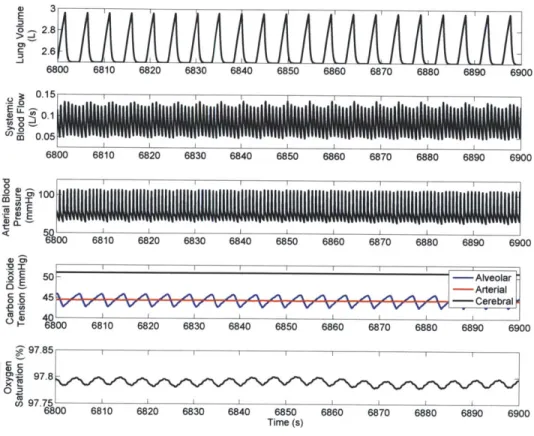
themselves in sleep, so it helps to consider how the simulation behaves when sleep is enabled and all other parameters are left at their default values. The generated waveforms should be roughly consistent with the time courses of physiological state variables in a normal individual exposed to a normal environment. Figure 2.2 shows the time courses of a few of PNEUMA's variables, under these conditions, during sleep.
( 31 o.22.8
I/l
005 6800 6810 6820 6830 6840 6850 6860 6870 6880 6890 6900 0 6800 6810 6820 6830 6840 6850 6860 6870 6880 6890 6900 078 5Z.6%00 6810 6820 6830 6840 6850 6860 6870 6880 6890 6900 0E 50- - Alveolar i5 E-Arterial j0N se enbe, [ CF1 sets up iCerebral
IP800 6810 6820 6830 6840 6850 6860 6870 6880 6890 6900 .Z97.85 II i >10 97.8 cin 97.75 6800 6810 6820 6830 6840 6850 6860 6870 6880 6890 6900 Time (s)
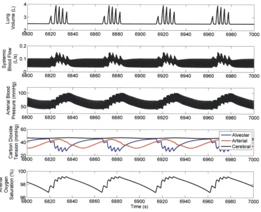
Figure 2.2: PNEUMA-simulated waveforms representing normal, steady conditions in sleep. Now, with sleep enabled, [CIFKlO] sets up its most extreme simulation of GSA as follows: " Reduce BaseEmaxlv - the parameter representing the basal maximum end-systolic elastance
of the left ventricle - by 90%, reflecting the severely diminished contractility of the left ventricle in a chronic heart failure sufferer. This results in severely diminished cardiac output . " Increase T_pdelay_const - the parameter representing the effective lung-to-carotid
trans-port volume' - by 50%, ostensibly to represent cardiomegaly, which is common among CHF
9 Increase Gp - the parameter representing the peripheral chemoreflex gain - by 600%, reflecting the elevation in hypercapnic ventilatory response that seems to be necessary for CHF sufferers to develop CSA.
The reduction in cardiac output and the increase in effective lung-to-carotid volume together increase the time delay that separates a change in blood gas levels at the pulmonary capillaries from the detection of the resulting change in blood gas levels at the carotid chemosensor site. Figure 2.3 shows the waveforms that result (once sleep has taken over) from simulating under these conditions.
400 6820 6840 6860 6880 6900 6920 6940 6960 6980 7000 0.2 1 0 c.2M 0L 6800 6820 6840 6860 6880 6900 6920 6940 6960 6980 7000 $ 50 d 6800 6820 6840 6860 6880 6900 6920 6940 6960 6980 7000 0 .0 E leoa 0iG 682 ia 98 % 00 6820 6840 6860 6880 6900 6920 6940 6960 6980 7000 Time (s)
Figure 2.3: PNEUMA-simulated waveforms representing CSA.
blood gas levels at the carotid bifurcation is taken equal to the effective lung-to-carotid transport volume divided by the instantaneous blood flow.
2.3
Issues with PNEUMA
PNEUMA is a very complex model with many parameters. The nominal values of many of these parameters have been drawn from published estimates that are interpreted as representing an "av-erage" subject. The remainder have been set by PNEUMA's developers, with the aim of generating behaviour in simulation that is "realistic" and "internally consistent". They judge the model's re-alism by comparing its responses under a variety of conditions to published empirical results that are taken to reflect "average" physiological behaviour in the population of interest. These compar-isons are almost entirely qualitative and generally examine only fairly coarse features of waveforms corresponding to a limited set of the model's state variables. The developers claim that a quantita-tive goodness-of-fit approach was not possible because no "single complete experimental dataset" is available for model validation.
In light of this, there are four principal issues with using PNEUMA as a model of CSA:
1. Validation: While its responses under the set of conditions studied may indeed look reason-able and the behaviours of its state varireason-ables may appear to be consistent with one another, PNEUMA has not been quantitatively validated against real data. It could hypothetically be the case that the developers' choices of parameter values result in a poor quantitative fit to real data, whether patient-specific or population-averaged, at baseline or in pathological conditions. Even if the subsystem models were each assigned parameter values that produced an acceptable fit to data used in the respective studies that developed these models, the inter-connection of such models may not yield an acceptable fit to new system-level data. It may be that, to obtain an acceptable fit, parameter values must be chosen outside the plausible ranges of the quantities they purportedly represent, or perhaps no choice of parameter values can give an acceptable fit. Such departures would indicate structural flaws in the model, such as missing or incorrectly-implemented components.
2. Minimalism: PNEUMA is in principle intended for the simulation of physiological behaviour under a wide variety of conditions. It may well be that much of its complexity is unnecessary for any specific purpose. For instance, the dynamics of very slow and very fast processes may not contribute to any of the phenomena of interest in CSA. The influence of fast dynamics (such
may be imperceptible over short recordings. It may be that a model that applies quasi-steady-state assumptions to fast-changing state variables and constancy assumptions to slow-changing variables would be perfectly adequate for explaining the phenomena that are of interest or manifest themselves in real data records. Some of PNEUMA's components may only significantly influence outputs that are neither measured in data records nor of interest in our study of CSA. Finally, some components (some of the branches of the ventilatory controller, for instance) may simply appear to be inactive in CSA (and perhaps in other conditions as well), possibly because their contributions to the response are small or change little relative to components that dominate the large- or small-signal response in this regime. PNEUMA's possibly-unnecessary complexity contributes significantly to the two items that follow.
3. Insight: By running simulations under a variety of conditions, patterns can be observed. For instance, the relative contributions of various parameters to system stability may be suggested. Because PNEUMA is so complex, each simulation takes a long time to run. Many simulations would need to be run to first propose and then confirm with some confidence any interesting patterns. No general conclusions may even be drawn in this manner, since parameter space cannot be explored exhaustively in simulation. Proposed patterns would need to be explained either analytically or intuitively, considering the model structure. However, the complexity of PNEUMA (many components, many interconnections, many nonlinearities, many parameters) renders analytical approaches and rigorous logical explanations all but impossible.
4. Identifiability: Consider some assignment of parameter values and the resulting "measured" output vector, obtained by concatenating the various measured outputs. Then there exists a region of parameter space for which the corresponding model output vector is very close (in a weighted sum of squares sense, say) to the measured output vector. If this region is just a fairly small neighbourhood in the parameter space, then there is hope of estimating the values of all parameters within some reasonable uncertainty. Otherwise, it is not possible to identify
the system in practice (using as a fitting cost function the same measure of output vector closeness as before). It may be, however, that some subset of the parameters can be selected such that the projection of the region mentioned before onto the corresponding restricted parameter space is just a fairly small neighbourhood. This restricted set of parameters could be estimated with some confidence. The remaining parameters do not contibute strongly enough to the output for their values to be estimable in practice; these could be set at their nominal values. Such non-identifiable parameters might, for example, be associated with the sorts of fast, slow, inactive, or unmeasured dynamics discussed previously.
Of these four issues, we now focus on the last: PNEUMA's identifiability. Ideally, we would want to answer the following questions for physiological data recorded as a single human subject experiences episodes of CSA:
1. Is it possible to assign values to parameters in PNEUMA so that the resulting simulated waveforms agree closely with their analogues in the real data record?
2. Can the parameter set be partitioned successfully into an identifiable subset and a non-identifiable subset? The non-non-identifiable parameters would all be assigned predetermined nominal or arbitrary values and we would only attempt to estimate the identifiable parame-ters to fit the model output to real data. A partition would be considered successful if
(a) demanding the best possible fit between simulated and real data restricted the iden-tifiable parameters to a tight region of the corresponding parameter space, which the implemented estimator would approach in reasonable time (i.e., the estimated parame-ters were in fact uniquely identifiable within acceptable uncertainty);
(b) the resulting identifiable parameter estimates would change little if the given real data were perturbed slightly, say through measurement noise (i.e., the estimator was robust); (c) simulated data generated using the estimated parameters would agree well with the given data (i.e., if, despite fixing a subset of the parameters at nominal values, bias was low). In the absence of real data, we resort to inspecting PNEUMA on its own. For if PNEUMA, with its parameters set to produce output data exhibiting episodes of CSA, cannot be identified accept-ably from noise-corrupted versions of its own output, then there is surely little hope of identifying
2.4
Preparing PNEUMA for Numerical Experiments
PNEUMA version 2.0 is a software package at whose heart lies the PNEUMA Simulink model. However, for user-friendliness, the model is not normally accessed directly. Instead, the user accesses the PNEUMA "control panel" and its children, which together form a graphical user interface (GUI) through which the user may adjust aspects of PNEUMA's configuration (essentially, this provides access to some of PNEUMA's parameters) and run simulations. This interface also provides access to displays of simulation progress and graphs of selected simulated waveforms.
While possibly acceptable for a rather limited exploration of the model, PNEUMA 2.0's native form is not suitable for our purposes. To investigate the model's indentifiability as well as for other numerical explorations, we require the ability to automatically run a large number of simulations - one simulation for each desired assignment of values to parameters - and collect the results. To this end, the following steps were taken:
1. The graphical user interface was no longer used.
2. Parameter values, previously set and adjusted through a number of MATLAB scripts and GUI-linked functions that directly modified the properties of model blocks, are now all assigned their nominal values in a single script. The model uses the parameter values that are in place at the beginning of the simulation.
3. Simulations are now configured and run directly by the scripts that need them, not through the control panel.
4. Data-logging blocks have been added to the model, capturing the full simulated time courses of many signals of interest. (Some were being tracked less directly in the original implementation and were plotted as the simulation executed.) The data thus collected can be processed, stored, and analyzed by scripts.
2.5
Sensitivity Analysis
To shed some light on the issues raised in Section 2.3, we will now examine how much influence each of PNEUMA's parameters has on the behaviour of the model system in the CSA regime. For our investigation, we probe this behaviour via two "output signals":
1. The continuous tidal volume waveform, VT (t):
The functional residual capacity (FR C) is the volume of air that remains in the lungs at the end of each expiration during unforced breathing. Let AVL (t) denote the lung volume in excess of FRC. This excess volume increases from FRC during inspiration, reaches a maximum value -the tidal volume - at -the end of inspiration, -then decreases back to FRC as air leaves -the lungs during expiration. At steady state in the CSA regime, we may construct a continuous periodic waveform, with period equal to the time between the beginnings of successive apneas, that fits the maxima of the AVL waveform and lies at zero during apneas. We call this waveform the continuous tidal volume waveform and denote it by VT (t). It represents the periodic envelope of the steady-state AVL waveform, and at the end of each inspiration, it approximates the tidal volume for that breath.
2. The arterial carbon dioxide tension, pa (t):
At steady state in the CSA regime, the partial pressure of carbon dioxide in the blood at the peripheral chemosensor site is very well approximated by a smooth periodic waveform, pa (t), having the same period as VT (t). We will refer to the common period of oscillation of VT (t)
and pa (t) as the CSA period, T.
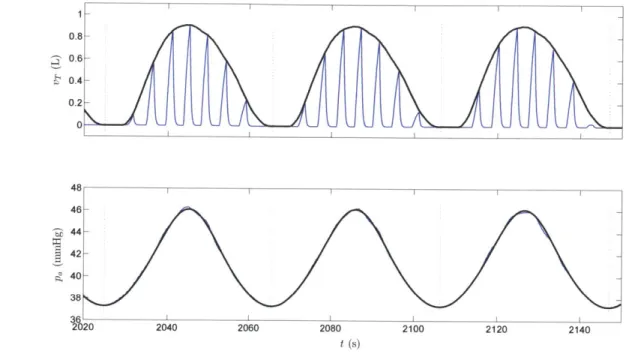
Figure 2.4 shows VT (t) and pa (t) over a few CSA periods for our prototypical PNEUMA CSA simulation.
0.6 0.4 0.2 48 46-, 542- 40-38 2020 2040 2060 2080 21OO 2120 2140 t (s)
Figure 2.4: The upper plot shows the AVL waveform (blue) generated in our prototypical PNEUMA CSA simulation, along with the corresponding fitted periodic VT waveform (black). The lower plot shows the arterial carbon dioxide tension waveform (blue) generated by PNEUMA, along with the corresponding fitted periodic pa waveform (black).
Recall that we are interested in those aspects of the model system's behaviour that are associated with the key phenomena that manifest themselves in typical data records of CSA cases. We have therefore chosen to observe the system's behaviour through quantities that exhibit neither high-frequency activity (associated with dynamics occurring on timescales shorter than the duration of one breath)2 nor very low-frequency activity (associated with phenomena that become apparent only over many cycles of CSA). Furthermore, note that we consider the model system's behaviour in steady-state.
2.5.1 Our Procedure
Our goal is to determine how strongly each model parameter influences VT and Pa at steady state in the CSA regime. We will do this by measuring how much these two waveforms change as a result of a small perturbation in each parameter.
2
For instance, we selected the tidal volume waveform rather than the lung volume waveform, and the arterial carbon dioxide tension rather than the alveolar tension.
We must therefore meaningfully quantify the difference between periodic waveforms that may have different periods. To this end, we now define finite-duration signals, j' and ', representing one period of Pa and VT, respectively. Let twin denote the time at one of the minima of the Pa (t) waveform. We then extract a segment of the Pa (t) waveform spanning one CSA period, bounded by a pair of adjacent minima, and we transform its time axis so that this segment spans the normalized time interval
[-,
{): Pa (T((+
-1) + ti .. for- <{ a (0) =2 0 elsewhere Similarly, VT(T
(+-1)+
t,,in) for -<g < .1 0 elsewhereTo compare Pa and VT waveforms obtained under different parameter configurations, we may directly
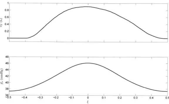
compare the corresponding a and o'' waveforms and CSA periods. Figure 2.5 shows the p'a and
6-waveforms corresponding to the Pa and VT waveforms shown in Figure 2.4.
0.4- 0.2-0 46 -- 0-'i44 42 -gi40 38 --.5 -0!4 -0 3 -0.2 -0.1 0 0!1 0.2 0!3 0!4 0.5
Figure 2.5: The & and G3 waveforms corresponding to the pa and VT waveforms shown in Figure 2.4.
We now describe the steps of our sensitivity analysis:
1. We first simulate the model system under our prototypical "baseline" CSA parameter values. From the resulting output waveforms, we determine To = T, G' (() = 6' (() and '' ( ) =
Pa
(),
which represent the steady-state behaviour of the model at baseline.2. We compile a list of M model parameters of interest: 01, 02,..., A, whose baseline values are 01,0, 62,o, ..., OM,o, respectively.
3. For each parameter, 9
k, k = 1,2, ... , M, in our list, we run a pair of simulations in which we
perturb 6k first 5 % downward (-), then 5 % upward (+):
(-)
We set 6k = 0.9 50 k,o and leave all other parameters (including those not in our list) at their baseline values, then simulate the model system. From the resulting output waveforms, we determine T_ = T, o (() = P (() and p (P ) = -().
(+)
We set 0k = 1.05 0k,o and leave all other parameters (including those not in our list) at their baseline values, then simulate the model system. From the resulting output waveforms, we determine Tk+ = T, ' (() = ' (() and p'k'+ ( ) = & (i).
4. To quantify the changes in the continuous tidal volume waveform resulting from the perturba-tions in 6k, we compute the RMS (root mean square) value of the difference between v3±
()
and ' (i), and divide it by the total swing in the baseline continuous tidal volume waveform to obtain the dimensionless quantity
S1~ =Tk TO d
Sv,k± = max jj7'
( )
- min1<<vo~Similarly, we define
Sp~k =max __
(< )
mm, i 1< <i PaO(Sv,k_ and Sv,k+ provide measures of the magntiude of the sensitivity of the continuous tidal volume to 9
k, while Sp,k- and Sp,k+ provide measures of the magntiude of the sensitivity of the
arterial carbon dioxide tension to 0
k. Since these sensitivities quantify changes in the single-period-normalized waveforms v__- (() and p'-±
( )
relative to baseline, we must consider the change in CSA period separately. We therefore introduce a third sensitivity measure:|Tk± - TO
For each k = 1, 2, ...
,
M, we take the senstivities Sv,k = max (So,k_, Sv,k+), Sp,k = max (Sp,k_, Sp,k+), and ST,k = max (ST,k_, ST,k+) to measure the influence 0k exerts on the behaviour of model system components of interest, on the timescales of interest, in the regime of interest.
2.5.2 Some Additional Details
Disabling the Sleep Mechanism
To perform our sensitivity analysis, we found it necessary to modify PNEUMA beyond the alter-ations described in Section 2.4: we disabled the sleep mechanism. The sleep state variables were instead held constant at values consistent with sleep. We took this step for two reasons:
the initial state of the system to represent a subject who is already very nearly asleep3, the process of sleep onset takes some considerable time, with the sleep state variables changing
significantly before finally reaching values that represent a sleeping subject.
2. The intact sleep mechanism causes the sleep state variables to change during sleep. We would then be unable to clearly identify a "typical" cycle of CSA for each parameter configuration, and the slow-timescale processes involved lie outside the scope of our study.
Excluded Parameters
We start with a candidate pool of parameters, made up of all the named quantities that are initialized in preparation for a PNEUMA simulation. (We therefore miss any initial conditions, saturation limits, gains, and other model component properties whose values are hardcoded in the PNEUMA Simulink implementation.) We will not investigate sensitivity to changes in all these parameters. In particular, we exclude the following from further consideration:
" all quantities that do not appear in the PNEUMA model (a very small minority of these are parameters rendered inert by our removal of the sleep mechanism);
" parameters associated with interventions such as Valsalva maneuvers or applied airway pres-sure;
" one parameter that represented a physical constant;
" parameters that control properties of the simulator, or data logging;
e binary-valued parameters; and
* parameters whose baseline values are zero, since we perturb each parameter in proportion to its baseline value.4
3
This does not appear to be a straightforward task.
4
We can recommend reasonable scales for some of these parameters, but for consistency, we do not include those results here.
In the end, we are left with M = 264 parameters, including those that specify initial conditions.
Baseline Configuration
The baseline parameter configuration we used differs somewhat from the prototypical CSA con-figuration discussed in Section 2.2: we reduced BaseEmaxlv by 70 % (instead of 90 %), and we increased Gp by 400 % (instead of 600 %). This milder configuration represents another of the cases mentioned in [CIFK10].
2.5.3 Results
We now present a summary of the results of our sensitivity study.
Having determined S,,k± and S,,k for k = 1,2,... , M, we rank the parameters according to S,,k. The parameter with the largest So,k is assigned rank R,,k = 1, the parameter with the second-largest S,,k is assigned rank R,,k = 2, and so on. Similarly, we assign ranks R,,k according to the values of Sp,k, and RT,k according to ST,k. Figure 2.6 plots the sensitivities So,k± and S,,k against the rank Rv,k for each parameter 9
k. Figures 2.7 and 2.8 show sensitivity-versus-rank plots for pa and T, respectively. 100 10 - v,k--o S ,k 10-2 0 50 100 150 200 250
50 100
Rp,k
150 200
Figure 2.7: Sensitivity versus parameter rank, for -p^.
50 100
RT,k
150 200
Figure 2.8: Sensitivity versus parameter rank, for T.
Witness that there are two parameters for which a 5 % perturbation leads to quite a significant 10
--
-k'
4 -2 103 10 L 0 250 100 10 102 10-3 104 10-10 -6 0 - STk o ST.k-Q -1 - I I 250-change in '. There are three parameters like this for &. Notice also that there is a clear gap separating the eleven highest Sv,k values from the rest, with no comparable gaps among these lower 253 Sv,k values. We will refer to the corresponding set of eleven parameters as the '-influential cluster. We see a similar gap separating the nine highest Sp,k values and the lower 255, among which no comparable gaps appear. We will refer to the corresponding set of nine parameters as the pa-influential cluster. Note that the gaps in Sv,k and Sp,k appear at similar values of these roughly normalized sensitivities. It is less easy to identify a cluster of most influential parameters in Figure
2.8, but one reasonable possibility is the set of parameters with the six highest ST,k values.
The twenty-six data points we have identified correspond to sixteen distinct parameters. Un-surprisingly, some parameters appear in more than one of the three clusters we have identified. The following parameters appear in both the '-influential cluster and the jij-influential cluster:
* all three gas level thresholds of the chemoreflex controller;
" the total blood volume;
* the effective lung-to-carotid volume; and
" one of the parameters that characterizes the (dissociation) mapping from oxygen and carbon dioxide partial pressures in the blood to blood oxygen concentration.
The sensitivities associated with the remaining parameters are very small indeed.
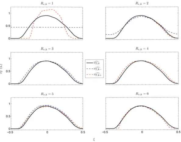
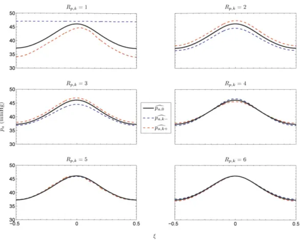
To better illustrate just how much or how little - and & change as a result of a 5 % change in each of the highest-ranked parameters, we show in Figure 2.9 the i17, o', and 'r k waveforms for the parameters with the six highest Sv,k values, and in Figure 2.10 the PaB , p and Pa+ waveforms for the parameters with the six highest Sp,k values.
R,k = 4 0.5. 0 1 0.5 0 1 0.5 0 0.5 -0.5 -- Tk - - VT,k+ R,,k = 6 0 0.5
Figure 2.9: Baseline and perturbed ' waveforms for the six highest-ranked parameters.
- - -
-R1,k = 5
Rp,k = 3 45 40 35 30 50 45 40 35 -p~ 5 rFn. 45 40 35 0
Figure 2.10: Baseline and perturbed p' waveforms for the six highest-ranked parameters.
Note the peculiar and extreme results of downward perturbations for the parameters with R,,k = 1, Rk = 2, and R,,k = 1. The parameter corresponding to R,,k = R,,k = 1 is the peripheral (arterial) chemoreflex threshold for oxygen. By decreasing its value by 5 %, we moved the system out of the CSA regime and into the stable regime, where VT and pa do not oscillate appreciably. The parameter ranked second in terms of its influence on ' represents the central chemoreflex threshold (for carbon dioxide). Once we decreased its value, breathing continued to be periodic, but apneas no longer appeared.
It is certainly possible that among the lower-ranked parameters, numerical factors can account for much of the difference observed between (ir'i and o' and between '' and p . Performing longer simulations might allow us to generate more accurate ' and p-a waveforms, and this may reduce the computed sensitivities. It is also important to note that PNEUMA includes few if any sources of non-numerical noise. Many of the output waveform changes we have observed would be
R,,k 1 R,,k = 2 -=- -- -Pa,k--P,k* 0.5 -0.5 0 0.5 I -Rp,k 4 Rpk = 6
In the vicinity of the parameter configuration we selected to represent CSA conditions, the tidal volume and arterial carbon dioxide tension waveforms appear to be insensitive to changes in the values of all but a few parameters. This lends support to the following hypotheses:
1. If, given only continuous tidal volume and arterial carbon dioxide tension waveforms collected in the CSA regime at steady state, we are able to successfully partition PNEUMA's parameters into an identifiable subset and a non-identifiable subset, the non-identifiable subset will be much larger than the identifiable subset.5
2. It is possible to construct a small model (one with few parameters and state variables) that can, in simulation, approximately reproduce the steady-state tidal volume and arterial carbon dioxide tension waveforms generated by PNEUMA in the CSA regime.
(It seems reasonable to expect that the role played here by the continuous tidal volume and arterial carbon dioxide tension waveforms would be similarly well played by any small set of waveforms representing intermediate-frequency activity of physiological state variables.)
The remainder of this thesis is dedicated to the development and analysis of a small grey-box model of central sleep apnea.
5
A New, Simple Model
3.1
Overview
A block diagram representing our model is presented in Figure 3.1.
Unlike PNEUMA, we will not be modelling processes that occur on timescales shorter than one breath. For example, we do not model the rise and fall of lung volume over the course of each breath. We instead propose a model that provides a plausible picture of system behaviour down to a resolution of around two to four breaths. We shall refer to this as our "multibreath" timescale. Our model also does not include processes on timescales longer than a few minutes -processes associated with changing sleep state or metabolism, for instance. If the model parameters (non-signal quantities) are treated as constants, then the model is applicable at most over intervals of time during which the general physiological state of the subject is approximately constant. Of course, it should be possible to separately model system behaviour in a number of general states (different sleep or metabolic states, say), by setting the model parameters appropriately in each case. If the parameters are instead viewed as slowly-varying exogenous variables whose waveforms may be supplied to the model, then longer simulations may become meaningful.
Ventilation Plant
4
.A--A
Pulmonary Gas Exchange Plant Lung-to-Carotid Transport Plant Cerebral Gas Exchange Plant d a.+ Periphieral Control Branch
d1
Central Control Branch Chemoreflex Controller
(a)
X1
x2
(d) Figure 3.1: (a) A blo
cal system P with inp x (t) and output y (t) put y (t) = x1 (t) + x2
y (t)
(0M
xt-XTHck diagram of our new, simple model, where (b) represents a dynami-ut x (t) and odynami-utpdynami-ut y (t), (c) represents a static gain element with inpdynami-ut
- Gx (t), (d) represents an adder with inputs x1 (t) and x2 (t) and
out-(t), and (e) represents a thresholding element with input x (t) and output if x(t) < XTH
if x (t) > XTH
3.1.1
Pulmonary Gas Exchange Plant,
PAWe model the pulmonary (or alveolar) gas exchange process as a single-input single-output (SISO) dynamic plant, PA'. The input to the plant is alveolar ventilation, denoted by
#A.
It represents the rate at which fresh air is brought into the alveoli for gas exchange. The plant's output is PA, the partial pressure of carbon dioxide in the alveolar spaces and in the pulmonary end-capillary bloodThe "A" stands for "Alveolar".
(b) (c) (e)