HAL Id: hal-03008090
https://hal.archives-ouvertes.fr/hal-03008090
Submitted on 15 Apr 2021
HAL is a multi-disciplinary open access
archive for the deposit and dissemination of
sci-entific research documents, whether they are
pub-lished or not. The documents may come from
teaching and research institutions in France or
abroad, or from public or private research centers.
L’archive ouverte pluridisciplinaire HAL, est
destinée au dépôt et à la diffusion de documents
scientifiques de niveau recherche, publiés ou non,
émanant des établissements d’enseignement et de
recherche français ou étrangers, des laboratoires
publics ou privés.
Joël J.-m. Hirschi, Bernard Barnier, Claus Böning, Arne Biastoch, Adam
Blaker, Andrew Coward, Sergey Danilov, Sybren Drijfhout, Klaus Getzlaff,
Stephen Griffies, et al.
To cite this version:
Joël J.-m. Hirschi, Bernard Barnier, Claus Böning, Arne Biastoch, Adam Blaker, et al.. The Atlantic
Meridional Overturning Circulation in High-Resolution Models. Journal of Geophysical Research.
Oceans, Wiley-Blackwell, 2020, 125 (4), �10.1029/2019JC015522�. �hal-03008090�
Joël J.‐M. Hirschi1 , Bernard Barnier2 , Claus Böning3, Arne Biastoch3 , Adam T. Blaker1 , Andrew Coward1 , Sergey Danilov4 , Sybren Drijfhout5, Klaus Getzlaff3,
Stephen M. Griffies6 , Hiroyasu Hasumi7 , Helene Hewitt8 , Doroteaciro Iovino9 , Takao Kawasaki7, Andrew E. Kiss10 , Nikolay Koldunov4 , Alice Marzocchi1 ,
Jennifer V. Mecking1, Ben Moat1 , Jean‐Marc Molines2, Paul G. Myers11 , Thierry Penduff2 , Malcolm Roberts8 , Anne‐Marie Treguier12, Dmitry V. Sein4 , Dmitry Sidorenko4 ,
Justin Small13, Paul Spence14 , LuAnne Thompson15 , Wilbert Weijer16 , and Xiaobiao Xu17
1National Oceanography Centre, Southampton, UK,2Université Grenoble Alpes, CNRS, IRD, Grenoble‐INP, IGE,
Grenoble, France,3Geomar, Kiel, Germany,4Alfred Wegener Institute for Polar and Marine Research, Bremerhaven,
Germany,5University of Southampton, Ocean and Earth Science, Southampton, UK,6Atmosphere & Ocean Sciences Program, NOAA/GFDL + Princeton University, Princeton, NJ, USA,7Atmosphere and Ocean Research Institute, The
University of Tokyo, Tokyo, Japan,8Met Office, Exeter, UK,9Ocean Modeling and Data Assimilation Division, Centro Euro‐Mediterraneo sui Cambiamenti Climatici, Italy,10Research School of Earth Sciences, Australian National University
+ ARC Centre of Excellence for Climate Extremes, Canberra, ACT, Australia,11Department of Earth and Atmospheric Sciences, University of Alberta, Edmonton, Alberta, Canada,12Laboratoire d'océanographie Physique et Spatiale,
CNRS, Brest, France,13NCAR/UCAR, Boulder, CO, USA,14Climate Change Research Centre, University of New South Wales + ARC Centre of Excellence for Climate Extremes, Sydney, New South Wales, Australia,15University of
Washington, School of Oceanography, Seattle, WA, USA,16Los Alamos National Laboratory, Los Alamos, NM, USA,
17Florida State University, Center for Ocean‐Atmospheric Predictions Studies, Tallahassee, FL, USA
Abstract
The Atlantic meridional overturning circulation (AMOC) represents the zonally integrated stream function of meridional volume transport in the Atlantic Basin. The AMOC plays an important role in transporting heat meridionally in the climate system. Observations suggest a heat transport by the AMOC of 1.3 PW at 26°N—a latitude which is close to where the Atlantic northward heat transport is thought to reach its maximum. This shapes the climate of the North Atlantic region as we know it today. In recent years there has been significant progress both in our ability to observe the AMOC in nature and to simulate it in numerical models. Most previous modeling investigations of the AMOC and its impact on climate have relied on models with horizontal resolution that does not resolve ocean mesoscale eddies and the dynamics of the Gulf Stream/North Atlantic Current system. As a result of recent increases in computing power, models are now being run that are able to represent mesoscale ocean dynamics and the circulation features that rely on them. The aim of this review is to describe new insights into the AMOC provided by high‐resolution models. Furthermore, we will describe how high‐resolution model simulations can help resolve outstanding challenges in our understanding of the AMOC.1. Introduction
The Atlantic Meridional Overturning Circulation (AMOC) is often defined as the zonally integrated and vertically accumulated meridional ocean volume transport in the Atlantic Ocean. The main reason why the AMOC has been the subject of many studies is because of its role in the climate system (e.g., Jackson et al., 2015; Stocker, 2013). The AMOC is a major contributor to the redistribution of heat from the low latitudes where there is a net heat gain owing to strong solar radiation to the higher latitudes where there is a net heat loss to the atmosphere. In the North Atlantic the AMOC transports about 0.5 PW across the equator, increasing to a maximum of 1.3 PW of heat northward at 26°N (Hall & Bryden, 1980; Johns et al., 2011; McCarthy et al., 2015; Baringer et al., 2018). As a result, the AMOC is thought to moderate the climate of western and northern Europe with effects felt well into Eurasia (e.g., Rahmstorf & Ganopolski, 1999).
©2020. The Authors.
This is an open access article under the terms of the Creative Commons Attribution License, which permits use, distribution and reproduction in any medium, provided the original work is properly cited.
Special Section: Atlantic Meridional Overturning Circulation: Reviews of Observational and Modeling Advances
Key Points:
• Observations and high‐resolution models have changed view on the AMOC pathways
• High‐resolution models suggest the presence of previously unknown high‐frequency AMOC variability • High‐resolution models allow to
estimate the intrinsic/chaotic component of the AMOC
Correspondence to:
J. J.‐M. Hirschi, [email protected]
Citation:
Hirschi, J. J.‐M., Barnier, B., Böning, C., Biastoch, A., Blaker, A. T., Coward, A., et al. (2020). The Atlantic meridional overturning circulation in high‐resolution models. Journal of Geophysical Research: Oceans, 125, e2019JC015522. https://doi.org/ 10.1029/2019JC015522 Received 24 JUL 2019 Accepted 20 JAN 2020
The paleoclimate record suggests that the AMOC is likely to have undergone major rearrangements in its structure between glacial and interglacial periods and has been subject to abrupt (i.e., multidecadal/centennial to millennial timescales) changes, as reviewed by Lynch‐Stieglitz (2017) and Moffa‐Sánchez et al. (2019). For instance, during the last glacial period from 115,000 to 11,700 years ago, Greenland Ice‐core records show repeated pronounced warming and cooling events (e.g., Dansgaard– Oeschger and Heinrich events; Heinrich, 1988; Dansgaard et al., 1993) that are superposed on the longer climate cycles from glacial cycles. Whereas the factors that caused these events are still unclear, analyses of multiple proxies have suggested a connection to the AMOC (e.g., Bond et al., 1999; Gebbie, 2014; Amrhein et al., 2018). A particularly interesting and important point raised in these studies is whether abrupt AMOC changes seen in the past may happen in the present or future climate.
The paleo record suggests that the AMOC may be subject to rapid change in strength and stability with con-sequent changes in AMOC‐related meridional heat transport (e.g., Jansen et al., 2018; Thornalley et al., 2018). Currently, climate projections suggest that the AMOC will weaken (but not collapse) in response to global warming (Drijfhout et al., 2012; Reintges et al., 2017; Stocker et al., 2014). However, whether the cur-rent generation of low‐resolution climate models adequately simulates the sensitivity of the AMOC to a warming climate is still a matter of debate (e.g., Caesar et al., 2018; Rahmstorf et al., 2015) with some authors suggesting that the sensitivity in nature could be higher than previously thought (Heuzé, 2017; Reintges et al., 2017). For more exhaustive overviews about the AMOC and mechanisms driving its strength and variability we refer the reader to comprehensive reviews such as Lumpkin and Speer (2007), Kuhlbrodt et al. (2007), Buckley and Marshall (2016), Zhang et al. (2019), Johnson et al. (2019) and Weijer et al. (2019). The observational quantification of the components of AMOC has included multiple efforts at different loca-tions within the Atlantic basin. Since the Meteor expedition in the 1920s, we have known that one can infer geostrophic transports across a section from the end points (e.g., Merz, 1925). Moored instruments at key locations at the basin margins are sufficient to estimate strength, vertical structure, and variability of geos-trophic transports between the end points of a mooring array line (e.g., Hirschi et al., 2003; Lee & Marotzke, 1998; Rayner et al., 2011). In the OVIDE program that began in 1997 hydrographic sections are used to quantify the transports between Greenland and Portugal (Mercier et al., 2015). The MOVE array began deploying moorings in 2000 that allow an estimate of the deep southward transport of AMOC at 14°N (Elipot et al., 2014; Kanzow et al., 2006).
Repeat hydrographic sections (observations of temperature, salinity, and depth) along with cabled measure-ment of the transport of the Florida Current in Florida Straits (e.g., Bryden et al., 2005) can give estimates of AMOC near 26°N. However, the infrequent hydrographic sections make it likely that AMOC variability inferred from such sections is aliased in time. Since 2004 a continuous observing system for the AMOC has been deployed in the North Atlantic across 26.5°N (Cunningham et al., 2007; Kanzow et al., 2007; McCarthy et al., 2012, 2015). This system provides estimates of the strength, variability, and vertical struc-ture of the AMOC (Smeed et al., 2014, 2018) and provided thefirst observational evidence that the AMOC can undergo substantial variations on short (i.e., subannual to interannual) timescales (Cunningham et al., 2007; Kanzow et al., 2007, 2010; McCarthy et al., 2012; Smeed et al., 2014, 2018; Bryden et al., 2014). In the framework of the SAMOC (South Atlantic Meridional Overturning Circulation) program, a combina-tion of different seccombina-tions, moorings, and satellite altimetry is used to provide estimates of strength and variability of the AMOC in the South Atlantic (e.g., Dong et al., 2009; Perez et al., 2011, 2015; Pérez et al., 2013). Using a variety of platforms, AMOC measurements at other latitudes and locations have been imple-mented in the last decade. OSNAP (Overturning in the Subpolar North Atlantic) provides a framework for estimating the AMOC in the subpolar North Atlantic since 2014 (Holliday et al., 2018; Lozier et al., 2017; Lozier et al., 2019).
At some latitudes AMOC time series have been extended through the combination of in situ measure-ments listed above along with Argo measuremeasure-ments and satellite altimetry that in some cases allows extending the measurements back to the beginning of the altimeter record in 1993 (e.g., Willis 2010, Frajka‐Williams, 2015, Mercier et al., 2015, and Perez et al., 2018). These measurements provide invalu-able information about the AMOC and are unique benchmarks against which models can be evaluated (e.g., Blaker et al., 2015; Duchez et al., 2014; Xu et al., 2014) at the corresponding locations. While this wealth of observations opens up the prospect of being able to understand how the ocean circulation and
the AMOC in particular impact Atlantic‐wide changes in properties such as heat, freshwater, and car-bon (Frajka‐Williams et al., 2019; Perez et al., 2018), the current observational network is not sufficient to study the full four‐dimensional spatiotemporal velocity structure that makes up the AMOC structure. How and on what timescales AMOC variability at different latitudes is related cannot yet be conclusively assessed from observational records.
Ocean models, ranging from simple box models to complex general circulation models, have informed our understanding of the mechanisms that drive the AMOC and its variability (e.g., Bingham et al., 2007; Böning et al., 2006; Robson et al., 2014). Box models with analytical or numerical solutions (e.g., Stommel, 1961; Marotzke et al., 1988; Griffies & Tziperman, 1995; Longworth et al., 2005; Wood et al., 2019; Alkhayuon et al., 2019) were and still are useful (and popular) tools to illustrate and study possible AMOC behavior. Within their limitations (spatial resolution, physical assumptions, parameterisation choice, etc.) general cir-culation models provide self‐consistent four‐dimensional data sets for the ocean circir-culation (including the AMOC); they allow us to“play” with different scenarios, test likely sensitivities in the climate system, in some instances they can guide observational efforts (e.g., Hirschi et al., 2003), and can point to currents and circulation features before these are observed in nature (e.g., Aksenov et al., 2011; Treguier et al., 2005). However, models inevitably have shortcomings in their ability to represent the physics of nature. In coarse‐resolution models (order 1° or coarser) currents, which are known to be jet like in the real ocean, are simulated as broad and diffuse currents with velocities much weaker than observed and they are often in the wrong location and have the wrong vertical structure. In addition, mesoscale ocean eddies as detected by satellite altimetry (Chelton et al., 2007) are not resolved. Nearly all the models included in the CMIP5 climate projections use coarse ocean model resolution.
In parallel to the increase in the availability of high‐quality AMOC estimates, there has been a massive increase in high‐performance computing (HPC) resources and in our ability to exploit them to simulate the natural world. The latest generation of ocean and coupled ocean‐atmosphere models is being run at reso-lutions sufficient to simulate the ocean circulation with a remarkable level of detail (e.g., Böning et al., 2016; Haarsma et al., 2016; Iovino et al., 2016; Marzocchi et al., 2015; Moat et al., 2016; Rieck et al., 2019; Sein et al., 2016, 2017). Features such as ocean mesoscale eddies are now increasingly present in ocean and ocean‐ atmosphere simulations. In some instances increased resolution results in better representation of boundary currents such as the Gulf Stream, the Agulhas‐, Brazil‐, and Malvinas currents (e.g., Biastoch et al., 2018; Griffies et al., 2015; Hewitt et al., 2016; Murakami et al., 2015; Sein et al., 2018; Small et al., 2014). Similarly, fronts, and the associated gradients of temperature and salinity, are more sharply defined. Improved representation of oceanic surface temperature gradients is of particular interest in coupled simu-lations, where the ability to simulate a more realistic imprint of the ocean onto the atmosphere is a potential source of improvement in forecasting systems. Satellite observations and reanalyses have shown that the ocean front associated with the Gulf Stream affects the atmosphere all the way up to the tropopause (Minobe et al., 2008; Minobe et al., 2010; Siqueira & Kirtman, 2016). In model simulations a similar effect is only found when the underlying ocean represents the sharp temperature front across the Gulf Stream (Kuwano‐Yoshida et al., 2010; Minobe et al., 2008). In addition, the presence of mesoscale eddies changes the character of the simulated variability across timescales (Penduff et al., 2010). The latest generation of coupled ocean‐atmosphere models now increasingly uses an ocean component that is “eddy permitting” (nominal 0.25° resolution) or in some instances“eddy rich” (Roberts et al., 2018, nominal 0.1° resolution). A noteworthy benefit that emerged from the use of a higher‐resolution model is found in seasonal forecast-ing where for thefirst time a significant skill is found for winter forecasts for the North Atlantic Oscillation (Dunstone et al., 2016; Scaife et al., 2014). However, the physical mechanisms for this breakthrough in sea-sonal forecasting are not yet clear. A major change in the model used to produce the forecasts was the use of an eddy‐permitting ocean model. The resulting improvement in the position of ocean currents and fronts in the North Atlantic is thought to play a key role. However, the representation of the dense overflow across the sill separating the European Nordic Seas from the subpolar North Atlantic remains a challenge owing to the small‐scale processes that control the interaction of small‐scale topography and entrainment into the overflow plume (Legg et al., 2009).
The goal of this review is to evaluate how ocean simulations in the eddying regime inform our understanding of the mean, structure, and variability of the AMOC. We emphasize that each level of complexity from very
simple, highly idealized (analytical and numerical) models to the latest state‐of‐the‐art high‐resolution numerical models that run on massively parallel HPC architectures can provide valuable insights in our quest to better understand the role of the AMOC in the global climate system. This review is structured as follows: Section 2 shows results from a set of high‐resolution models to illustrate how the AMOC is represented in this latest generation of models. Section 3 focuses on the insight gained from studying AMOC in high‐resolution models. Section 4 summarizes areas in need of improvement. Finally, section 5 outlines areas where high‐resolution simulations can inform future research. Finally, a brief conclusion is given in section 6.
2. AMOC in High‐Resolution Models: Where Do We Stand?
More than three decades have passed since the pioneering regional and global eddying ocean simulations were performed (Semtner & Chervin, 1988; Semtner & Mintz, 1977). Owing to computational cost, these early eddying simulations were run for short periods. The integration length was sufficient to develop the mesoscale eddyfield and sharp boundary currents but too short for studies of quantities, such as the AMOC, that require that the deep ocean circulation is allowed to adjust. Furthermore, to keep computational cost manageable, these simulations used a relatively small number of vertical levels, and the main focus was on the surface circulation. Thesefirst efforts at high‐resolution ocean modeling were followed by programs such as the Fine Resolution Antarctic Model (The FRAM GROUP, 1991; Stevens, 1991; Killworth, 1992; Lutjeharms et al., 1995), the Ocean Circulation and Climate Advanced Modelling Project (Saunders et al., 1999; Webb et al., 1997; Webb et al., 1998), the Family of Linked Atlantic Model Experiments (Dengg et al., 1999), the Parallel Ocean Program (Maltrud et al., 1998; Smith et al., 2000), the CLIPPER Project (Treguier et al., 1999), and the Miami Isopycnic Coordinate Ocean Model (Paiva et al., 1999). Both integration length and vertical resolution were increased in these modeling efforts, allowing studies of eddy statistics, cir-culation structure, and variability in the Southern Ocean (e.g., Stevens, 1991; Killworth, 1992; Lutjeharms & Webb, 1995), the North Atlantic (e.g., Böning & Herrmann, 1994; Eden & Willebrand, 2001; McCLean et al., 2002; Böning et al., 2003; Treguier et al., 2005), or the Pacific (e.g., Richards et al., 2006). During the last dec-ade or so, there has been a consolidation of the modeling efforts mentioned above with longer simulations (multidecadal and sometimes even longer) that are eddy rich and even ensembles performed at eddy‐ permitting or eddy‐rich resolutions (e.g., Bessières et al., 2017; Iovino et al., 2016; Marzocchi et al., 2015). These simulations also use a higher number of vertical levels/layers. Whereas early high‐resolution ocean models were all run in ocean‐only mode, significant efforts have been and are being dedicated to coupling eddy‐permitting and increasingly eddy‐rich ocean components to an atmosphere model (e.g., Delworth et al., 2012; Griffies et al., 2015; Haarsma et al., 2016; Hewitt et al., 2016; Ito et al., 2015; Roberts et al., 2019; Winton et al., 2014). This coupling allows the community not only to address questions around the ocean cir-culation and its variability but also to refine our understanding of how, where, and on what timescales the ocean interacts with the atmospheric circulation and vice versa.
In this review, we use output from a large (but not exhaustive) set of state‐of‐the‐art high‐resolution ocean‐ only and coupled ocean‐atmosphere simulations to examine how these models represent the AMOC and its variability (Table 1). Multimodel intercomparisons of the AMOC have been done before (e.g., Danabasoglu et al., 2014) but not for high resolution (i.e., eddying models). The goal here is not to provide an in‐depth multimodel intercomparison but to use output from current high‐resolution models to provide an overview of the range of solutions obtained for the AMOC.
The AMOC (ψ) is calculated from the model velocity fields as follows: ψð Þy;ζ ¼ ∫
xe xwdx∫
η
z x;y;ζð Þdz′v x; y; z′ð Þ;
where v is the meridional velocity component; xe, xware the eastern and western limits of the zonal
integra-tion; andη is the free surface height. The lower limit, z(x,y,ζ), can denote a geopotential level (ζ = z) or the depth of any sea water property such as sea water density referenced to a given pressure (e.g.,ζ = σ2) (Hirst
et al., 1996; Nurser & Lee, 2004; Zika et al., 2012; Danabasoglu et al., 2014). As the focus of this review is the AMOC this integration is limited to the meridionally bounded portion of the Atlantic Basin (including the Mediterranean and Baltic Seas) with the southernmost point of the Cape of Good Hope. In the remainder of this review we will refer to the AMOC in depth and density coordinates asψ(z) and ψ(σ2), respectively.
Table 1
Overview of the High‐Resolution Simulations Used to Illustrate Aspects of the AMOC in this Review
Model (institute)
Grid spacing (deg) and grid Ocean
only Coupled Regional Global Integrations Reference (s)
Horiz. Vert.
FESOM (AWI) Unstructured
0.25–1 48 X X 1948–2007 (COREII) Danilov et al. (2004) Sein et al. (2016, 2017, 2018) Unstructured 0.1–0.6 48 X X 1948–2007 (COREII) Unstructured 0.25–1 48 T63 X 1950–2099 Unstructured 0.1–0.6 48 T63 X 1950–2099
CESM‐H (NCAR) 0.1 62 CAM5
0.25
X 100 years
(year 2000 forcing)
Small et al. (2014, 2018)
ACCESS‐OM2‐1 1 50 (z*) X X 300 years (five repeats
of JRA55‐do 1958–2017)
Kiss et al. (2020)
ACCESS‐OM2‐025 0.25 50 (z*) X X 300 years (five repeats
of JRA55‐do 1958–2017)
ACCESS‐OM2‐01 0.1 50 (z*) X X 33 years (JRA55‐do
1985–2017) HYCOM 0.08 hybrid iso/sig/z X X Xu et al. (2012, 2013, 2014) NEMO‐ORCA (MEOM Team, Uni Grenoble) 0.25 46 X X 327 years (normal year) Grégorio et al. (2015) Bessières et al. (2017) Leroux et al. (2018) 0.25 75 X X 50 × 1958–2015 (DFS5.2) 0.25 75 X X 330 years (normal year) 0.083 75 X X 1958–2007 (DFS4.4) NEMO‐VIKING20X (GEOMAR) 0.05 46 X X (nested Atl.) X (global 0.25) 1958–2009 (COREII) Böning et al. (2016) Rieck et al. (2019) 0.05 46 X X (nested Atl.) X (global 0.25) 1980–2018 (JRA55‐do) 0.25 46 X X (global 0.25) 1958–2016 (JRA55‐do) NEMO ANNA0083 (Uni Alberta) 0.083 50 X X (20S to Bering Strait) X 2002–2018 Müller et al. (2017) Courtois et al. (2017) Hu et al. (2018) NEMO‐ORCA (NOC‐UK Met
Office) 0.083 75 X X 1958–2015 (DFS5.2) Marzocchi et al., 2015 Hewitt et al. (2016) Moat et al. (2016) Roberts et al. (2019) 0.25 75 N216 X 300 years 0.083 75 N512 X 1950–2050 (year 1950 forcing) MIROC (AORI‐Uni
Tokyo) 0.25 63 T85 X >6,000 years (normal year) Tatebe et al. (2019) COCO 1 X 1958–2015 (JRA55‐do) 1 X >500 years (normal year) 0.25 X >100 years (normal year) 0.17 X 1958–1979 (cont.) (JRA55‐do)
0.17 X >100 years (PI run)
Note. Note that some low‐resolution versions are also included as these allow us to better assess improvements/changes seen at high resolution. Ocean‐only simu-lations are forced with the reanalysis products CORE II (e.g., Griffies et al., 2009), DFS (Brodeau et al., 2010), and JRA55‐do (Tsujino et al., 2018).
A variety of simulations is analyzed to explore the range of AMOC solutions that are possible when mesos-cale eddies are represented. We focus onψz in a range of models with resolutions ranging from 1/20°
(VIKING) to 2° (ORCA2) (listed in Table 1). Both forced and coupled models are included, and, in some instances, the modeling system is run at different resolutions and/or different surface forcings. Most models are global, but two are configured for the Arctic‐North Atlantic (ANHA) or Atlantic‐Arctic Basins (VIKING). We also include, in some cases, the low‐resolution counterpart to highlight changes that are likely owing to an increase in resolution.
2.1. Dependence of the Mean AMOC on Resolution
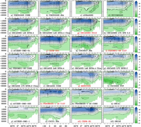
The range of solutions for the AMOC is quite broad, and within the eddy‐rich models the strength varies by almost a factor of 2 between the strongest and the weakest circulations (Figure 1). Similar results were found for the diversity of mean AMOC by Danabasoglu et al. (2014) in a comparison of low‐resolution forced simu-lations. The strongest AMOC cells are found in the eddy‐rich coupled models CESM‐H01, FESOM01‐06, and ORCA0083‐N512. Where comparisons can be made (ORCA0083, FESOM, and MIROC), we also find that the coupled version of the model produces a stronger AMOC than the forced ocean‐only configurations. The difference between coupled and uncoupled is most pronounced for FESOM. The reasons why a stronger AMOC is simulated in coupled simulations are not fully understood. However, stronger air‐sea interactions with increasing resolution are a plausible cause for stronger AMOC (and of the related meridional heat transport) in high‐resolution models (e.g., Grist et al., 2018; Roberts et al., 2016).
Figure 1. (a–z3) AMOC stream functions in depth coordinates in models from noneddying to eddy‐rich simulations. The highest resolutions are shown in the top row and lowest resolutions in the bottom row which are included for comparison. For properties of the models, see Table 1. Coupled ocean‐atmosphere models are indicated in red.
Quantitative metrics for AMOC can be defined allowing comparisons among the models (Figure 2). South of about 35–40°N, the maximum overturning strength ψ(z) max (i.e., the maximum value of ψ
occurring in the water column for each latitude) in eddy‐rich models is on average about 3–4 Sv stron-ger than in the eddy‐permitting and noneddying models listed in Table 1 (Figure 2a). Between the equa-tor and about 35°N, the AMOC strength is nearly constant with latitude and eddy‐rich models simulate the largest AMOC strengths. To a lesser extent, this plateau is also seen for the eddy‐permitting models. Between 35–40°N and 50°N, there is a sharp decrease in ψ(z)maxfor the eddy‐rich models to about 60% of the
value at 26°N (Figure 2a). This decrease is a bit less pronounced in the eddy‐permitting models and at 50°N ψ(z)maxis about 70% of its 26°N value. A different picture characterizesψ(z)maxin the noneddying models.
On average the maximum AMOC strength also occurs between 25°N and 40°N but the sharp decrease seen for the high‐resolution model is not seen at coarser resolution. At 50°N the ψ(z)maxin the noneddying models
is still about 90% of its 26°N value and the sharpest decrease inψ(z)maxoccurs north of about 55–60°N
(Figure 2b). We will return to this difference between eddy‐rich/permitting and noneddying models and its meaning in terms of AMOC pathways in section 3.
To compare with a larger set of low‐resolution models, Figure 2 also shows ψ(z)maxobtained from a large
subset of 29 models from the Climate Model Intercomparison Project phase 5 (CMIP5). For the CMIP5 mod-elsψ(z)maxis noticeably stronger than for the low‐resolution models listed in Table 1. South of about 35°N
ψ(z)maxis only marginally lower than for the eddy‐rich models. However, the latitudinal dependence of the
AMOC strength in CMIP5 models is very similar to that in our set of coarse‐resolution models (CMIP5 curve has similar shape but is shifted upward by ~3 Sv). The CMIP5 models show the same behavior as the low‐ resolution models discussed here, but the average of the 29 models is offset by about 3 Sv from the average of the models discussed here. In the CMIP5 modelsψ(z)maxalso reach its highest values between about 25°N
and 45°N and at 50°Nψ(z)maxis more than 90% of the value at 26°N. It is worth noting here that most
CMIP5 models were tuned toward a realistic AMOC strength. No such tuning was done for the high‐ resolution models presented here. Apart from the horizontal resolution the high and low versions were
Figure 2. (a–c) Maximum overturning (ψ(z)) as a function of latitude for eddy‐rich, eddy‐permitting, and noneddying models. Solid lines show the average maximum AMOC strength and shading indicates ±0.5 standard deviation. The CMIP5 values included for comparison are based on 29 models: ACCESS1‐0, ACCESS1‐3, BCC‐CSM1‐1, BCC‐CSM1‐1‐m, CanESM2, CCSM4, CESM1‐BGC, CESM1‐CAM5‐1‐FV2, CESM1‐CAM5, CESM1‐FASTCHEM, CESM1‐WACCM, CMCC‐CESM, CMCC‐CM, CMCC‐CMS, CNRM‐CM5‐2, CNRM‐CM5, CSIRO‐Mk3‐6‐0, EC‐EARTH, FGOALS‐g2, GFDL‐ESM 2G, GFDL‐ESM 2M, GISS‐E2‐R‐CC, GISS‐E2‐R, HadCM3, HadGEM2‐AO, HadGEM2‐CC, HadGEM2‐ES, IPSL‐CM5A‐LR, IPSL‐CM5A‐MR, MRI‐CGCM3, MRI‐ESM 1, NorESM1‐ME, NorESM1‐M (see, e.g., Mecking et al., 2017 for more details about these models).
kept as similar as possible. This suggests that the sharp decrease inψ(z)maxbetween 26°N and 50°N in high‐
resolution models compared with low‐resolution models is a robust feature.
The eddy‐rich models have the strongest MHT (meridional heat transport) with the highest values occurring between about 15°N and 35°N (Figure 2b). Only marginally weaker values are found for the eddy‐permitting models, while the MHT is clearly lower in low‐resolution models. Consistent with ψ(z)max, the MHT is
clearly higher in the CMIP5 ensemble than for the low‐resolution models listed in Table 1. South of about 20°N, the MHT is very similar in CMIP5 and in the eddy‐rich models. North of about 25°N, the MHT is slightly lower than in the eddy‐rich models but the differences are not large. For MHT the shapes of the curves are more similar between low‐ and high‐resolution models than for the MOC curves shown in Figure 2a. For latitudes north of about 30°N some CMIP5 models get similar MHT values than eddy‐rich models but Figures 2a and 2b suggest that the relative contributions of overturning and gyres are different in the CMIP5 models than in the eddy‐rich models and that noneddying models may get the “right” MHT transport for the wrong reason.
Another feature that is apparent is a deepening of the AMOC cell at eddy‐rich resolutions compared to the eddy‐permitting and noneddying models as defined by the vertical structure of ψ(z) at 26°N (Figure 2c). However, all of the model AMOC cells are too shallow compared to observational estimates (Figures 1 and 2c; Lumpkin & Speer, 2007). Profiles of ψ(z) at 26.5°N where a comparison with the RAPID observations can be made show very good agreement in the top 2,000 m (Figure 2c). However, below 2,000 m the modeled AMOC values are lower than the observation‐derived transports, which suggests that the southward return flow of the AMOC simulated at depth is shallower than in observations. However, there is an improvement over the noneddying forced simulations (discussed in Danabasoglu et al., 2014) in the strength of the south-wardflow. In the CMIP5 models ψ(z)maxat 26°N is too deep but the southward returnflow for ψ(z) occurs at
depths that are too shallow (indicated by the more rapid decrease ofψ(z) with depth than in the observations or the eddy‐rich models). The vertical extent of the AMOC cell looks very similar in z‐level models and HYCOM, which uses hybrid coordinates (Figure 1). One could perhaps expect that hybrid coordinates would favor a deeper overturning cell than z‐levels but this is not the case here. This result was also seen in the lower‐resolution hybrid coordinate model used in Danabasoglu et al. (2014).
There is an indication that the AMOC slightly deepens in the model configurations using a higher number of vertical levels—for example, ORCA0083 with either 46 or 75 vertical levels. The effect is not pronounced though, and it is not clear how robust it is as the coupled version of ORCA0083 (which also used 75 vertical levels) has a marginally shallower AMOC cell than the forced ORCA0083 version. It is worth remembering that the AMOC from RAPID is obtained from density observations and using the thermal wind relation to infer geostrophic velocities. Whereas there is strong evidence that the RAPID approach leads to a good esti-mate of the“true” AMOC strength and variability (e.g., Hirschi et al., 2013; Sinha et al., 2018), the “true” AMOC could conceivably fall between the models and the AMOC estimate from RAPID.
To illustrate the impact of increasing the horizontal resolution, Figure 3 shows the differences between high‐ and low‐resolution models for ψ(z) where both versions of the model (using the same forcing fields or atmo-spheric model) are available. The differences between eddy‐rich and noneddying configurations all show an increase in the strength of the NADW cell in the eddy‐rich models. This is strongest for ORCA and ACCESS with an increase of the overturning cell by up to 8–10 Sv. Smaller increases between 2 and 6 Sv are seen for CESM‐H and COCO. The latter also shows a significant increase in the strength of the AABW cell at depth. In COCO the strengthening of the NADW cell is confined to the top 2,000 m, whereas positive anomalies reach down to about 3,500 m for ORCA, ACCESS, and CESM‐H. Much smaller differences are found for FESOM (both forced and coupled) where positive anomalies are confined to depths between about 1,500 and 4,000 m. These smaller differences for FESOM are not unexpected since both the high‐ and low‐ resolution versions are eddying, that is, eddy rich (FESOM01‐06) and eddy permitting (FESOM025‐1). A fea-ture which can also be seen in all but one case (ACCESS) is weak negative overturning anomalies north of about 40°N which is consistent with the similar or slightly higher overturning values simulated by low‐ resolution models at high latitudes (Figure 2a).
It is important to acknowledge that the AMOC strength and vertical structure are very sensitive to surface forcing. The models included in this review do not allow us to systematically assess the influence of the
surface forcing. We made opportunistic use of available high‐resolution model output, and no attempt was made here to either compare models using the same surface forcing to many different models (e.g., as in Danabasoglu et al., 2014) or to systematically assess the impact of using different surface forcings. Nevertheless, the surface forcing in the models included here (Table 1 and Figure 1) either uses a range of forcings: CORE, DFS, JRA, and CGR over differing time periods or they are coupled ocean‐atmosphere models. Forcing differences may explain some of the range of the AMOC solutions. The range of solutions we present here is consistent with earlier studies of both low‐resolution (e.g., Danabasoglu et al., 2014) and high‐resolution (e.g., Behrens et al., 2013) models.
3. What (Knowledge) Have We Gained?
In this section we highlight key improvements that have been made in the representation of the AMOC as resolution is increased.
3.1. AMOC Pathways
High‐resolution ocean simulations have contributed to our understanding of how and on what spatial and temporal scales the AMOC can exhibit variability. Both observations and the models highlight that the pic-ture of a global conveyor belt, a termfirst coined by Broecker (1987) and subsequently often used to describe the global meridional overturning circulation, is a very much simplified view (Lozier, 2010). The picture of a conveyor as well as that of a meridionally coherent overturning circulation stream function, as illustrated in Figure 1, only emerges when averaging velocities over several years or longer. Any snapshot (or averaging on timescales shorter than about monthly) of the AMOC reveals the much more intricate, complex nature of the ocean circulation. Currents implied to be coherentflows in AMOC schematics can be seen to consist of a suc-cession of eddies andfilaments (with some coherent jets in places such as the Gulf Stream between Florida and Cape Hatteras; e.g., Hirschi et al., 2019). For surface currents, this picture is confirmed in both satellite observations and in high‐resolution ocean models and for many features there is remarkable agreement between observations and model simulations (Figure 4). In particular the Florida Current and Gulf
Figure 3. AMOC differences between the high‐ and low‐resolution versions of ACCESS, CESM‐H, COCO, and ORCA. Contour interval is 2Sv.
Stream are well represented in the high‐resolution simulations with the path of the Gulf Stream separating at Cape Hatteras in high resolution but hugging the coast well past Cape Hatteras in the low‐resolution simulations (Chassignet & Marshall, 2008; Danabasoglu et al., 2014). In addition, the path of the North Atlantic Current is qualitatively well represented in the high‐resolution simulations. This is thought to be a key region for modulating decadal variability in low‐resolution simulations (Buckley & Marshall, 2016). The eddy‐rich circulation is not confined to the surface, but the velocity field at greater depths also shows similarly intricate circulation features (albeit with lower velocities, Figures 4c and 4f). Modeled current velo-cities reveal interior pathways resembling observations from Lagrangianfloats (Figure 4c; Bower et al., 2009, 2011). These interior pathways are thought to be signatures of eddy‐driven recirculation gyres (Lozier, 1997, 1999), as shown in both hydrographic data and eddy‐permitting and eddy‐rich simulations, which represent key routes for the export of Labrador Sea Water into the subtropical North Atlantic (Gary et al., 2011; Lozier et al., 2013). South of the equator, the structure of the DWBC also becomes dominated by eddies (Figure 4c), as observed around 8°S (Dengler et al., 2004), before splitting into two pathways further south, one continu-ing along the continental shelf and the other spreadcontinu-ing in the interior of the basin (Garzoli et al., 2015). The improvements in the position and strength of currents are reflected in integral quantities as well. The vertically integrated transport of the subpolar gyre (SPG) strongly depends on resolution (Figure 5). In the models used for this review the SPG is stronger at eddy‐rich resolutions with maximum values of 30–50 Sv in the Labrador and Irminger Seas with a shape consistent with observations (Treguier et al., 2005; Colin de Verdière & Ollitrault, 2016; Figure 5f). The SPG also extends southward along the coast of North America with a narrow wedge reaching Cape Hatteras, consistent with the separation of the Gulf Stream at Cape Hatteras (Figures 5a–5c). A vigorous SPG is still simulated at eddy‐permitting resolution, but the position of the intergyre boundary shifts northward (especially off Cape Hatteras) and the narrow wedge
Figure 4. (a–f) Absolute velocities in cm/s from AVISO (geostrophic velocities) and ORCA0083 (ORCA0083‐N512). Weekly and annual averages are shown at surface for AVISO (from year 2007); 5‐day and annual averages are shown at the surface and 1,000‐m depth for the model solution (from model year 2007).
toward Cape Hatteras disappears (not shown). It is worth noting that Colin de Verdière and Ollitrault (2016) acknowledge that while their approach yields realistic gyre shapes, the quantitative stream function values are likely to be unreliable in the interior of the gyres. Compared to the eddy‐rich models, the barotropic stream function of Colin de Verdière and Ollitrault (2016) is weaker in the SPG and stronger in the subtropical gyre.
At noneddying resolutions the SPG is weaker (10–20 Sv maximum) in particular in the western SPG (Figures 5d and 5e). However, only a limited number of low‐resolution simulations are used for comparison here. In the literature there are examples of low‐resolution models that exhibit vigorous SPG circulations of 30–45 Sv (e.g., Danabasoglu et al., 2014; Yeager et al., 2015). However, as for the AMOC, low‐resolution mod-els exhibit a large range of values for the maximum SPG strength (Danabasoglu et al., 2014; their Figure 16) with the majority of models simulating an SPG strength between 15 and about 30 Sv. It is noteworthy that the version of ACCESS (1°, CORE forced) used in Danabasoglu et al. (2014) has a vigorous (~35 Sv) circula-tion, but in ACCESS‐OM2‐1 the SPG strength is only 10–20 Sv which suggests a large sensitivity to forcing and parameter choices. Neither of the high‐resolution simulations used in this review nor any eddy‐rich simulations we are aware of reported a weak SPG circulation—despite different forcings, coupling to differ-ent atmospheres, or differdiffer-ent parameter choices. This suggests that a vigorous SPG of realistic strength is a robust feature of eddy‐rich simulations.
The changes in the representation of the SPG (more realistic currents around Greenland/Labrador and strength) have implications for how currents project on the AMOC in depth and in density coordinates (Figure 6). Only when the zonally integrated meridionalflow is nonzero is there a projection onto the AMOC in depth coordinatesψ(z); a gyre circulation with compensating northward and southward flows along its western and easternflanks does not project onto ψ(z). In density coordinates, both overturning and gyre transports project ontoψ(σ2) as long as compensating volume transports occur in different density
classes. The SPG strongly projects ontoψ(σ2) as it is characterized by a large density contrast between the Figure 5. The barotropic stream function in the North Atlantic (Sv) averaged over the last 30 years of the simulations for high and low resolutions: (a) ORCA0083, (b) ACCESS‐OM2‐01, (c) HYCOM0083, (d) ORCA025, and (e) ACCESS‐OM2‐1. (f) Barotropic stream function from Colin de Verdière and Ollitrault (2016) inferred from Argo displacements,
predominantly northward transport in the eastern SPG and the returnflow along Greenland and Labrador in the western SPG (e.g., Lherminier et al., 2007).
The AMOC cell in depth coordinatesψ(z) weakens markedly north of about 30–40°N in eddy‐rich simula-tions (illustrated for VIKING005 and ACCESS‐0M2‐01 in Figure 6). This is indicative of significant sinking between middle and high latitudes. At low resolutions, the sharpest weakening ofψ(z) occurs close to the northern limit of the overturning cell, which is illustrated in Figure 6 for ORCA2 and ACCESS‐OM2‐1 and Figure 2a. Previous studies have shown similar differences betweenψ(z) in high‐ and low‐resolution models (e.g., Treguier et al., 2006; Marsh et al., 2009; Katsman et al., 2018), suggesting that in low‐resolution models a larger fraction of the sinking occurs at the northernmost latitudes ofψ(z) in low‐resolution models than in high‐resolution models.
The weakening of the AMOC cellψ(z) between middle and high latitudes seen at high resolutions is indica-tive of a change in the dominant AMOCflow pathways north of about 40–50°N. This can be illustrated by comparing the shapes for the AMOC in depth and in density coordinates (Figure 6). The overturning max-imum is consistently found at higher latitudes forψ(σ2) thanψ(z), but this difference is more pronounced at Figure 6. Schematic of main AMOC pathways at high resolution with vigorous SPG (top left), low resolution and weak SPG (top middle) as well as“classic” conveyor‐type pathway as expected in, for example, box models (top right) Colors (red to blue) indicate the gradual cooling and density increase of water masses along the AMOC path. AMOC in depth (second row) and potential density referenced to 2,000‐dbar (third row) coordinates for two
high‐resolution (VIKING005, ACCESS‐OM2‐01) and low‐resolution (ORCA2, ACCESS‐OM2‐1) simulations. Bottom row: maximum values ofψ(z) (blue) and ψ(σ2) (black).
high than at low resolution (Talandier et al., 2014). This is consistent with the stronger SPG simulated at high resolution, with warm and salty waters from the North Atlantic Currentflowing northeastward and forming the easternflank of the SPG. These waters are less dense than the colder, fresher southward flowing waters along Greenland and the Labrador Shelf in the western SPG.
The stronger SPG and more realistic current pathways at high resolutions means that these transports of contrasting water masses project strongly onψ(σ2). The highest values ofψ(σ2) occur between about 50°N
and 60°N in high‐resolution models (Figure 6, columns for VIKING005 and ACCESS‐OM2‐01), and ψ(z) is only about half the strength of ψ(σ2). In contrast, at low resolution the maximum values for
ψ(σ2) are reached at similar latitudes as found in high resolution, but at these latitudesψ(z) in low resolution
is 70–80% of ψ(σ2). The low‐resolution versions of VIKING/ORCA (NEMO) and ACCESS‐OM2 have a
weaker SPG when compared to other low‐resolution models. However, a strong SPG in a low‐resolution model does not necessarily mean high subpolar values for ψ(σ2). Low‐resolution models (e.g.,
Danabasoglu et al., 2014; Zhang, 2010) consistently show a smaller difference between ψ(z) and ψ(σ2) north of about 30°N than for the high‐resolution examples shown in Figure 6 (or in other studies such
as Grist et al., 2012). In Zhang et al. (2010) the maximum MOC strength, in this low‐resolution simulation with a relatively strong SPG, is only marginally weaker in depth (20–22 Sv) than in density coordinates (24 Sv) and the latitudes where the highest AMOC values occur overlap. The same is true for the larger low‐resolution model ensemble studied in Danabasoglu et al. (2014) where the results show that the values ofψ(z) are at least 70–80% of those seen for ψ(σ2) between about 40°N and 60°N (comparing their Figures 3
and 4). In the examples shown in Figure 6 it is only north of about 50°N that the maximum values ofψ(σ2)
and ψ(z) diverge at low resolution, whereas differences start at about 35°N for the eddy‐rich models (Figure 6, bottom). For the high‐resolution models the values of ψ(z) between 40°N and 60°N are only about 50% ofψ(σ2) suggesting a stronger gyre contribution toψ(σ2).
The impact of the difference in the pathways between high‐ and low‐resolution models and their impact to the AMOC are illustrated in Figure 5. For very coarse, 2‐D models or box‐models, the AMOC circulation is close to the“classic” conveyor type with water masses moving northward, sinking (over a relatively small range of latitudes) and returning south at depth. At coarser, noneddying resolution, the AMOC no longer purely consists of its overturning component. There is also a weak gyre contribution symbolized by a little loop at the northern end of the conveyor schematic (Figure 5). At high resolution, there is a clear horizontal loop at high latitudes symbolizing a vigorous SPG (which projects onψ(σ2) but notψ(z)). This change in
pathways is also linked to changes in the location of the sinking. Whereas at low resolutions sinking occurs mainly in the central Labrador and Irminger Seas, it is concentrated along the northern and westernflanks of the SPG at eddy‐permitting resolutions (Katsman et al., 2018).
3.2. AMOC Variability and Stability
Since 2004 AMOC observations at 26°N have shown variability on timescales ranging from submonthly up to what we have observed (e.g., Smeed et al., 2018). From models and observations we know that the AMOC likely varies on subdaily to millennial timescales and longer. In this section we will focus on aspects of the AMOC variability and AMOC features that have either beenfirst described in high‐resolution models or studies in which high‐resolution models have shed new light. For more general discussions on the AMOC variability and on the underlying mechanisms the reader is referred to Buckley and Marshall (2016).
3.2.1. Overview of Subdaily to Decadal AMOC Variability
The AMOC variability found in high‐resolution models on different timescales is illustrated with the stan-dard deviation of the overturningψ(z) (Figure 7). By far the largest variability occurs on the shortest time-scales (subdaily to daily). We note that seeing the highest variability on short timetime-scales is not specific to high‐resolution models; this is true for low‐resolution models as well. However, especially on very short timescales (subdaily to perhaps weekly) high‐resolution models have been shown to exhibit AMOC variability which has not been reported from low‐resolution models (e.g., Blaker et al., 2012). Additionally, the presence of eddies adds chaotic‐intrinsic variability on a range of timescales which is not present at low resolution (e.g., Hirschi et al., 2013; Grégorio et al., 2015; Leroux et al., 2018; see also section 3.2.2). The highest standard deviations of 40–50 Sv are centered within a few degrees of latitude around the equator. Standard deviation values away from the equator are much lower albeit still substantial (maximum of 7–8 Sv). This latitudinal variability structure is maintained when the AMOC variability is
computed from daily or 5‐day averages, but the maximum values reduce to about 20 and 5 Sv at equatorial and extraequatorial locations. For the timescales of up to 5 days the depth of the maximum variability is around 2,000 m for most latitudes. The pronounced equatorial variability maximum disappears when using monthly or longer timescales, but the largest variability still occurs in the equatorial region with values of about 5–6 Sv. However, these values no longer stand out as clearly compared to the maximum values of 3–4 Sv found away from the equator. The equatorial maximum is no longer seen when the variability is computed from annual means, and the largest values of 1–2 Sv are now seen in the North Atlantic between 20°N and 50°N. This meridional variability structure remains broadly similar when computing the AMOC variability from decadal means, but the values are reduced with maxima of about 1 Sv.
The presence of large AMOC variability in high‐resolution ocean models has been known for a number of years. In fact, models suggested the presence of a large (peak‐to‐peak of more than 10 Sv within a few months) midlatitude AMOC variability on subannual to interannual timescales (e.g., Baehr et al., 2004; Hirschi et al., 2003) before thefirst direct AMOC observations confirmed that variability of that magni-tude exists in the real ocean (Cunningham et al., 2007; McCarthy et al., 2012). Models also suggested that westward propagating features are not only key to the adjustment of the long‐term basin‐wide density gradients but that they can also cause subannual to interannualfluctuations of basin‐wide zonal density (and pressure) gradients that project onto the geostrophic component of the AMOC (e.g., Köhl, 2005; Hirschi et al., 2007; Cabanes et al., 2008). A particular benefit from models is the ability to use them to study how local AMOC estimates (i.e., across given sections as in RAPID or OSNAP) can be interpreted in a wider spatial context (Biastoch et al., 2008; Bingham et al., 2007; Hirschi et al., 2013). Although this
Figure 7. Standard deviation of AMOC (Sv) across a range of models. The standard deviations shown are computed from 4‐hourly, daily, 5‐daily, monthly, yearly, and decadal averages. The panels are arranged with the variability obtained from the highest temporal resolution (top left, 4‐hourly) to the lowest temporal resolution (bottom row, 10 years). Between 0 and 2 Sv the contour interval is 0.2 Sv, from 2–10 Sv it is 1 Sv, and from 10–40 Sv it is 10 Sv.
can also be done using low‐resolution models, high resolution is desirable because at low resolution boundary waves mediating AMOC changes are poorly represented due to poor representation of the continental shelf and key currents such as western boundary currents are too diffuse with velocities that are too low.
A recent interesting aspect revealed in high‐resolution ocean simulations is the suggested presence of pre-viously unknown types of AMOC variability. The very high AMOC variability found on subdaily timescales (Figure 7) was initially unexpected but was subsequently shown to be caused by the passage of near‐inertial waves triggered by wind variability at middle to high latitudes (Blaker et al., 2012). The magnitude of this AMOC variability is large (e.g., standard deviation of 7–8 Sv and peak‐to‐peak of up to 50 Sv at 26°N). To date, no observations exist to confirm the existence of such a near‐inertial AMOC variability in the real ocean. However, near‐inertial gravity waves are known to be ubiquitous in the world ocean and their presence has been confirmed by numerous observations (e.g., Alford, 2003; Alford et al., 2016). They have also been simulated in different ocean models (Fox et al., 2000; Komori et al., 2008), and theoretical considerations sug-gest that the AMOC may have a resonance at near‐inertial timescales (Sevellec et al., 2013). Whether near‐ inertial gravity waves do indeed project onto the AMOC in nature is not yet known. What we can say, though, is that if they do exist in nature, then these AMOC oscillations would be invisible to the RAPID (or OSNAP) observing systems. The near‐inertial impact on the AMOC is found in the nongeostrophic component, and direct velocity measurements across the full sections would be required to capture it.
Even larger variability (peak‐to‐peak of 400 Sv, standard deviation >50 Sv) has been found around the equa-tor (Hirschi et al., 2013). The dominant timescales of these oscillations are between 5 and 10 days, and they are caused by the wind variability in the equatorial region projecting onto baroclinic modes linked to equa-torially trapped near‐inertial waves. Similar to the near‐inertial AMOC oscillations mentioned earlier (Blaker et al., 2012), there is no observational evidence yet that such a high equatorial variability exists in nature. However, the mechanisms through which this high‐frequency AMOC variability occurs in high‐ resolution ocean models are known to exist, even if it is currently unknown whether they can project onto the AMOC as strongly as the models suggest. Even in models, it is currently unclear whether these large
Figure 8. Hovmoeller diagram ofψ(z) at 995‐m depth (top) and ψ(σ2) at 36.53 kg/m3 (bottom) as a function of time and latitude from 4‐hourly averages in an ORCA025 simulation. Units are Sv.
high‐frequency AMOC oscillations play a role on climate timescales. It is conceivable that they could enhance vertical mixing and hence affect the mean ocean state (and mean AMOC strength). However, at this stage it is equally possible that these oscillations—even though very large—are just “sloshing” water around without much interaction with the mean circula-tion and little consequence for climate. Note that these high‐frequency AMOC features project on both ψ(z) and ψ(σ2) (Figure 8). Numerous
observational studies show that near‐inertial gravity waves are ubiquitous in the ocean (e.g., Alford et al., 2016), and sea surface height variability shows variability on timescales consistent with the large equatorial AMOC variability (Durland & Farrar, 2012; Farrar & Durland, 2012) so the large high‐frequency AMOC variability simulated in high‐resolution ocean models may well be real. This is illustrated using output from an ORCA025 simulation where 4‐hourly averages are available for a 6‐month period. The presence of a clear variability signal inψ(σ2) suggests that,
even if not yet demonstrated, an impact on diapycnal mixing is plausible.
3.2.2. Eastern Versus Western Subpolar AMOC Variability
An important feature of the AMOC was recently revealed by the OSNAP observations in the subpolar North Atlantic. The AMOC esti-mate obtained from the first 21 months of observations from the OSNAP line suggests that the largest fraction of the AMOC variability on monthly timescales originates from the eastern part of the section with little AMOC variability coming from the Labrador Sea (Lozier et al., 2019). This time series provides a new benchmark against which we should test models. Many previous studies have looked at the importance of the Labrador Sea on the AMOC and its variability (e.g., Böning et al., 1996, 2006; Pickart & Spall, 2007; Robson et al., 2014; Rahmstorf et al., 2015; Feucher et al., 2019). What emerges from these studies is the likely importance of Labrador Sea processes for the AMOC and its variability on decadal or longer timescales. However, a recent analysis by Li et al. (2019) revealed that ocean models at eddy‐ permitting resolution and coarser are generally biased by an overpro-duction of Labrador Sea Water compared to observations, which tends to strengthen the AMOC response to changes in the volume of this water mass. Furthermore, the relationship between AMOC and Labrador Sea Water properties was found to degrade considerably downstream of the basin (Li et al., 2019).
In the context of this review, we examine the respective contributions from the eastern and western parts of the OSNAP sections in one of the latest coupled high‐resolution mod-els (ORCA0083‐N512). As in OSNAP, the transports are calculated in density coordinates and the AMOC is split into an eastern and western AMOC (Figure 9a). The transports shown are either monthly averages (Figure 9b) or smoothed with a 5‐year running average (Figure 9c). For monthly values the amplitude of the variability is similar for the eastern and western subpolar North Atlantic. Both the eastern and western AMOC transports are significantly correlated with the total subpolar AMOC, but the correlation is stronger for the eastern AMOC (r = 0.81) than for the western AMOC (r = 0.65). This means that a larger fraction (65%) of the variance has its origin in the eastern subpolar North Atlantic, but the variability contribution from the Labrador Sea is far from negligible (42% of variance). The 21‐month record presented in Lozier et al. (2019) shows almost no AMOC variability originating from the western part of the section. Nevertheless, the model supports the view that the AMOC contribution from the eastern subpolar North Atlantic plays an important role in the total AMOC variability. The model time series are much longer than the observational record (21 months). Figure 9c shows that a high correlation between the eastern AMOC transport and the total AMOC is maintained on decadal timescales with correlations similar between the total AMOC and the eastern and western transports (both >0.9). The model simulation suggests that
Figure 9. (a) Location of the eastern and western parts of the OSNAP sec-tion. (b) Left: maximum AMOC transports (MOC east/west) across the western and eastern OSNAP sections in ORCA0083‐N512 (control simula-tion). Shown is the AMOC across the full OSNAP section (blue), the western (red), and eastern (green) parts of the section. Right: MOC east versus MOC (top) and MOC west versus MOC (bottom). The time series are shown for the last 8 years of the simulation, and the scatter plots show monthly values for the 76 years of the simulation (1950 to 2026). (c) Same as (b) but for the whole length of the simulation and for transportfiltered with a 5‐year running average. Note that (as in OSNAP) different densities are used for the western, eastern, and full sections. Therefore, the sum of the eastern and western transport is not equal to the transport for the full section.
based on monthly values, the dominance of the east Atlantic on the subpolar AMOC variability is found throughout the simulation (Figure 9b), but on decadal timescales both eastern and western transports contribute approximately equally to the total AMOC (Figure 9c). Such analysis suggests that the respective contributions from eastern and western subpolar North Atlantic to the total AMOC should form a routine model performance metric (as, e.g., the AMOC at 26.5°N), calculated on a variety of timescales.
3.2.3. Chaotic/Intrinsic AMOC Variability
In the early days of RAPID AMOC observations, concerns were raised that the variability in the AMOC observations from RAPID could essentially consist of noise related to ocean mesoscale eddies and that “Real‐time detection of secular changes in the oceanic overturning circulation by regional measurements is probably a mirage” (Wunsch, 2008). Subsequent observation‐based studies did show that the noise level is much lower than what Wunsch (2008) suggested (Kanzow et al., 2009) and that the signal‐to‐noise ratio is much more favorable to the detection of long‐term trends in the AMOC by observing its evolution at one latitude. Nevertheless, AMOC observations show that the AMOC variability on short timescales is large and mesoscale features contribute to this variability.
Mesoscale eddies are the most intense and best known source of chaotic/intrinsic variability in the ocean: their phase is indeed inherently random and they spontaneously emerge in the ocean under steady forcing. Mesoscale kinetic energy peaks at relatively small time and space scales as eddies develop, but their mutual interactions subsequently feed chaoticfluctuations at larger space and timescales through spatial and tem-poral inverse cascades (Arbic et al., 2014; Sérazin et al., 2018). Other nonlinear processes such as large‐scale baroclinic instability, distinct from those occurring at the mesoscale, may also coexist with mesoscale instabilities (Huck et al., 2015) and feed multidecadal ocean chaotic variability with a substantial impact on the AMOC (Sévellec & Fedorov, 2013).
A systematic quantification of the impacts of atmospheric variability and intrinsic/chaotic processes on the AMOC variability is very difficult to obtain from observations alone. Different strategies using eddy‐permit-ting/rich simulations have been proposed to quantify these two impacts. Biastoch, Böning, and Lutjeharms (2008), for instance, compared two global simulations where eddies were (i) unresolved everywhere and (ii) resolved in the Agulhas region via a local grid refinement. The results show that resolving eddies in the Agulhas region triggers the emergence of a chaotic/intrinsic AMOC variability reaching interannual to dec-adal timescales and extending far into the North Atlantic. However, this local grid refinement did not allow nonlinear processes to generate chaotic/intrinsic AMOC variability at other latitudes of the Atlantic. The features and contribution of chaotic/intrinsic AMOC variability emerging in fully turbulent basins have been studied by forcing global ocean models at 2°, 1/4°, and 1/12° resolution by a repeated seasonal atmo-spheric forcing devoid of any interannual variability (Grégorio et al., 2015). Almost no interannual AMOC variability spontaneously emerged in the laminar 2° simulation, but a large amount of chaotic/intrinsic variability emerged at 1/4° and 1/12°, with comparable imprints on the AMOC. This chaotic/intrinsic AMOC variability was shown to reach multidecadal timescales and the scale of the Atlantic and to account at 35°S for half of the interannual‐to‐decadal variability found in fully forced hindcasts (simulations driven by the full range of atmospheric timescales—i.e., via an atmospheric reanalysis).
Estimating the relative contributions of the chaotic/intrinsic processes and of the atmospheric variability in the AMOC variability requires ensemble ocean simulations, where all members are driven by the same atmospheric conditions but are started from different initial conditions (as done by, e.g., Hirschi et al., 2013; Penduff et al., 2014; Bessières et al., 2017; Leroux et al., 2018). Note that the different eddyfields between ensemble members mean that air‐sea fluxes will also differ as they depend on the local ocean conditions.
Small perturbations to the initial conditions are sufficient to cause the AMOC variability to diverge between different ensemble members. This behavior is illustrated in Figure 10 for the spread of the AMOC at 26.5°N in a small ensemble performed with ORCA0083 forced with interannual data from DFS5.2. A six‐member initial condition perturbation ensemble of NEMO ORCA0083, created by advancing the simulation restart by one tofive model time steps, shows how the AMOC at 26°N, 1,000‐m depth, diverges under identical atmospheric conditions. (Figure 10). Note that as the eddyfield diverges between ensemble members, air‐ seafluxes will also diverge as the different eddy fields change the local ocean conditions. The ensemble begins on 1 April 2009, from the control simulation. The initial condition perturbations are very small,
and the model AMOC does not diverge for around 30 days. Between 30 days and 6 months, the ensemble diverges. All ensemble members broadly follow the same evolution, and the same dominant peaks and troughs occur in each ensemble member (Figure 10a). However, there is a spread of the AMOC time series around the ensemble mean. This spread is smaller than the variability in the ensemble mean (Figure 10a). The differences from the ensemble mean show that after 6 months the ensemble spread reaches saturation, with a (time mean) standard deviation of 1.1 Sv (Figure 10b). This is 27% of the standard deviation of the ensemble mean (4.15 Sv) which is consistent with Hirschi et al. (2013) (who also used 5‐day averages) and Grégorio et al. (2015) and Leroux et al. (2018) (who used monthly and annual averages). In this case the ensemble spread can be interpreted as the contribution of chaotic/intrinsic processes (including mesoscale eddies and larger chaotic anomalies) to the AMOC variability, and the temporal variability of the ensemble mean AMOC provides the atmospherically forced variability. These ensemble statistics confirmed that most of the chaotic AMOC variance remains strong up to multidecadal scales and that the phase of the broadband AMOCfluctuations around the ensemble mean remained random between each ensemble member (Leroux et al., 2018). In other words, the atmospheric variability only paces part of the AMOCfluctuations, while a significant part of the interannual‐to‐decadal AMOC variance conserves its chaotic character under a reanalyzed forcing. About 50% of the AMOC at 35°S is chaotic/intrinsic falling to typically 20–30% in the North Atlantic up to about 40°N and less than 10% in the subpolar region (Grégorio et al., 2015; Hirschi et al., 2013; Leroux et al., 2018). The reasons for these differences are far from understood yet, but the ensemble simulation strategy can provide some insight into the chaotic/intrinsic processes driving the AMOC fluctuations and into the atmospherically forced origin of certain AMOC anomalies observed in the RAPID time series or elsewhere (Leroux et al., 2018). However, given their large computational cost, large‐ensemble global simulations have only been
Figure 10. (a) Time series of the 5‐day mean AMOC at 26°N and 1,000‐m depth for a six‐member NEMO ORCA0083 ensemble. Start of all ensembles is 1 January 2009. Two ensemble members cover 1 year (January 2009 to December 2009) and four ensemble members cover 5 years (January 2009 to December 2014). (b) Deviation of the AMOC from the ensemble mean (Sv). The shaded regions in both panels indicate 1 and 2 standard deviations. For clarity, individual members are not plotted beyond 18 months.
performed at the coarser end of eddying resolutions (Bessières et al., 2017) or with small ensemble sizes and over short integrations (Figure 10). They nevertheless demonstrate that observed AMOCfluctuations cannot be only attributed to atmospheric forcing. The“eddy noise” propagates to much larger spatiotemporal scales, and as a result the predictability of the AMOC should be reevaluated in the presence of intrinsic ocean tur-bulence. However, in coupled simulations, eddies can be partly damped by atmosphericfluxes and as a result, eddy variability tends to be larger in forced models (Ma et al., 2016). Furthermore, intrinsic coupled climate variability from processes such as El Niño is also present in coupled models that can create addi-tional low‐frequency variability.
3.2.4. AMOC (Bi)stability
One of the key questions in AMOC research, namely, whether the AMOC can exhibit multiple stable states under identical surface boundary conditions, emerged from an analytical 2‐box model (Stommel, 1961). Since then the possible existence of multiple AMOC states, the likely conditions required for such multiple states to exist and for the AMOC to rapidly transition from one state to another in the real world, has been at the center of many studies. Multiple states have been obtained in wide range of available models: from ana-lytical models (e.g., Marotzke et al., 1988; Longworth et al., 2005) to complex three‐dimensional ocean‐only (e.g., Deshayes et al., 2013) and coupled models (e.g., Hawkins et al., 2011; Jackson & Wood, 2018; Manabe & Stouffer, 1988; Mecking et al., 2016). Despite such efforts, we can still not conclusively answer whether mul-tiple AMOC states (and in particular rapid transitions between these states) and related AMOC hysteresis could exist in the real world (e.g., Gent, 2013, 2018; Stocker, 2013). The possibility that the AMOC may have more than one equilibrium, and that a transition to this other equilibrium could be triggered by a large enough perturbation (e.g., a fresh water pulse from the Greenland ice sheet e.g. Weijer et al., 2012), has been a key research question for climatologists for decades; a collapse of the AMOC would have significant cli-mate implications, with large societal repercussions. Despite the potentially high impact, there is still signif-icant uncertainty in the likelihood of such an event (see Weijer et al., 2019 for a review).
Models with low resolutions such as those used in CMIP5 suggest a low probability for an AMOC shut-down under global warming scenarios (Collins et al., 2013). However, it has been suggested that sys-tematic biases in the salinity distribution of the Atlantic may overestimate the stability of the AMOC in these models (Liu et al., 2017; Mecking et al., 2017). A critical argument revolves around a metric called Fov, which is the freshwaterflux across 34°S in the South Atlantic due to the AMOC. In most low resolution models the AMOC imports freshwater into the Atlantic (Fov > 0), which would consti-tute a negative, stabilizing feedback (the so‐called salt advection feedback; e.g., Rahmstorf, 1996) on the strength of the AMOC: A weakening of the AMOC would reduce the freshwater import, salinifying the Atlantic, hence resisting a further weakening. Observations, however, suggest that the Fov < 0 at 30°S (e.g., Bryden et al., 2011; McDonagh & King, 2005; Weijer et al., 1999), which would suggest a positive, destabilizing feedback. Several model studies (e.g., de Vries & Weber, 2005; Weber & Drijfhout, 2007) show a surprising ability of the sign of Fov to predict whether the AMOC is in a regime of multiple equilibria (Fov < 0) or not (Fov > 0). Other studies (e.g., Dijkstra, 2007; Huisman et al., 2010) have refined this metric by including the AMOC‐induced freshwater transports at the northern boundary of the Atlantic, hence proposing a divergence indicator,Σ Fov. However, caution is warranted in inter-preting the negative sign of Fov (orΣ Fov) in observations as a sign of AMOC bistability. For one, the validity (or accuracy) of Fov as a stability indicator has been questioned, as modeling studies suggest that the freshwater transport by the wind‐driven gyre circulation may be at least as important as that of the AMOC in shaping the transient response to a large freshwater perturbation (Thomas & Fedorov, 2019; Gent, 2018; Mecking et al., 2016; Spence et al., 2013). But the more relevant question for this review is whether the AMOC stability paradigm—and the role of Fov—carries over from eddy‐parameterized to eddy‐rich models.
It is encouraging that high‐resolution models appear to simulate the correct sign of Fov at 30°S (Deshayes et al., 2013; Mecking et al., 2016). This would give credence to the suggestion that the Fov in low‐resolution models is biased positive due to model errors or poorly resolved processes (e.g., Agulhas Leakage; Weijer & Van Sebille, 2014). Experimentation with eddying models should reduce concerns that the stability of the AMOC is compromised by biases in the salinityfield.
But one question that needs to be addressed is whether the salt advection feedback, which is a critical ingre-dient for AMOC bistability, is active and effective in high‐resolution models. If this feedback is somehow