Impact of oceanic circulation changes on atmospheric δ 13 CO 2

HAL Id: hal-01805158

https://hal.archives-ouvertes.fr/hal-01805158

Submitted on 5 May 2021

HAL is a multi-disciplinary open access

archive for the deposit and dissemination of

sci-entific research documents, whether they are

pub-lished or not. The documents may come from

teaching and research institutions in France or

abroad, or from public or private research centers.

L’archive ouverte pluridisciplinaire HAL, est

destinée au dépôt et à la diffusion de documents

scientifiques de niveau recherche, publiés ou non,

émanant des établissements d’enseignement et de

recherche français ou étrangers, des laboratoires

publics ou privés.

L. Menviel, A. Mouchet, K. Meissner, F. Joos, M. England

To cite this version:

L. Menviel, A. Mouchet, K. Meissner, F. Joos, M. England. Impact of oceanic circulation changes on

atmospheric δ 13 CO 2. Global Biogeochemical Cycles, American Geophysical Union, 2015, 29 (11),

pp.1944 - 1961. �10.1002/2015GB005207�. �hal-01805158�

Impact of oceanic circulation changes on atmospheric

𝛿

13

CO

₂

1_{Climate Change Research Centre, University of New South Wales, Sydney, New South Wales, Australia,}2_{ARC Centre of}

Excellence for Climate System Science, Sydney, New South Wales, Australia,3_{Laboratoire des Sciences du Climat et de}

l’Environnement, IPSL-CEA-CNRS-UVSQ, Gif-sur-Yvette, France,4_{Department of Astrophysics, Geophysics and}

Oceanography, Université de Liège, Liège, Belgium,5_{Climate and Environmental Physics, Physics Institute, and Oeschger}

Centre for Climate Change Research, University of Bern, Bern, Switzerland

Abstract

2measured in Antarctic ice cores provides constraints on oceanic and terrestrial carbon

cycle processes linked with millennial-scale changes in atmospheric CO2. However, the interpretation of

𝛿13_CO

2is not straightforward. Using carbon isotope-enabled versions of the LOVECLIM and Bern3D models,

we perform a set of sensitivity experiments in which the formation rates of North Atlantic Deep Water (NADW), North Pacific Deep Water (NPDW), Antarctic Bottom Water (AABW), and Antarctic Intermediate Water (AAIW) are varied. We study the impact of these circulation changes on atmospheric𝛿13_CO

2as well

as on the oceanic𝛿13_{C distribution. In general, we find that the formation rates of AABW, NADW, NPDW,}

and AAIW are negatively correlated with changes in𝛿13_CO

2: namely, strong oceanic ventilation decreases

atmospheric𝛿13_CO

2. However, since large-scale oceanic circulation reorganizations also impact nutrient

utilization and the Earth’s climate, the relationship between atmospheric𝛿13_CO

2levels and ocean

ventilation rate is not unequivocal. In both models atmospheric𝛿13_CO

2is very sensitive to changes in AABW

formation rates: increased AABW formation enhances the transport of low𝛿13_{C waters to the surface and}

decreases atmospheric𝛿13_CO

2. By contrast, the impact of NADW changes on atmospheric𝛿13CO2is less

robust and might be model dependent. This results from complex interplay between global climate, carbon cycle, and the formation rate of NADW, a water body characterized by relatively high𝛿13_C.

1. Introduction

Recent technological advances now allow stable carbon isotope measurements in CO2bubbles trapped in

Antarctic ice sheets (𝛿13_CO

2).𝛿13CO2has been measured across the deglaciation and the Holocene in Taylor

Dome [Smith et al., 1999], EPICA Dome C [Elsig et al., 2009; Lourantou et al., 2010], and Talos Dome ice cores [Schmitt et al., 2012], thus providing strong constraints on carbon cycle changes occurring in the terrestrial and oceanic reservoirs during that time [Indermühle et al., 1999; Brovkin et al., 2002; Joos et al., 2004; Elsig et al., 2009; Menviel and Joos, 2012; Schmitt et al., 2012]. However, due to the number of processes possibly impact-ing atmospheric𝛿13_CO

2on millennial timescales, the interpretation of changes in𝛿13CO2can prove difficult

[Broecker and McGee, 2013]. For example, the ∼0.3‰𝛿13_CO

2decrease measured during Heinrich stadial 1 has

been attributed to enhanced Southern Ocean ventilation [Lourantou et al., 2010; Tschumi et al., 2011; Schmitt

et al., 2012], reduced iron fertilization [Lourantou et al., 2010; Broecker and McGee, 2013], and weakened North

Atlantic Deep Water (NADW) formation [Schmittner and Lund, 2015].

Carbon isotope fractionation occurs primarily during photosynthesis and air-sea gas exchange (Figure 1), while fractionation during carbonate precipitation is usually small [Turner, 1982]. In the ocean, the largest fractionation occurs during photosynthesis, when the light isotope (12_{C) is preferentially incorporated into}

organic matter, thus leaving dissolved inorganic carbon enriched in the heavy isotope (13_{C). Due to the}

sub-sequent remineralization of low𝛿13_{C organic matter at depth, deep ocean𝛿}13_{C is 1 to 2‰ lower than the}

surface ocean (Figure 1).

Numerical experiments performed with box models, and models of intermediate complexity can help con-strain the impact of different terrestrial and oceanic processes on atmospheric𝛿13_CO

2. Reduced terrestrial

carbon lowers𝛿13_CO

2by about 0.1‰ per 135–200 GtC [Joos et al., 2004; Brovkin et al., 2007; Köhler et al.,

2010; Elsig et al., 2009; Menviel and Joos, 2012]. Previous studies have shown that as fractionation between atmospheric CO2 and dissolved inorganic carbon (DIC) is temperature dependent [Zhang et al., 1995],

lower sea surface temperature increases the magnitude of the fractionation by 0.12‰ per degree Celsius,

RESEARCH ARTICLE

Key Points:

• Enhanced AABW decreases atmospheric𝛿13CO₂

• Changes in NADW formation rate have a small impact on𝛿13CO2

• Ventilation changes affect the global climate, which also impact𝛿13CO2

Supporting Information: • Text S1 Correspondence to: L. Menviel, [email protected] Citation:

Menviel, L., A. Mouchet, K. J. Meissner, F. Joos, and M. H. England (2015), Impact of oceanic circulation changes on atmospheric𝛿13CO₂, Global Biogeochem. Cycles, 29, 1944–1961, doi:10.1002/2015GB005207.

Received 5 JUN 2015 Accepted 26 OCT 2015

Accepted article online 2 NOV 2015 Published online 24 NOV 2015

©2015. American Geophysical Union. All Rights Reserved.

Figure 1. Mean preindustrial𝛿13C distribution (‰) and main processes influencing𝛿13C with an estimated isotopic difference (𝜖, gray oval). In the inserted graph, the zonally averaged surface ocean𝛿13C (blue lines) as well as the zonally averaged𝛿13C resulting from an isotopic equilibrium with the atmosphere (black lines) are shown for the preindustrial control run of LOVECLIM (solid) and the Bern3D (dashed). On land, a signature indicative of C3 plants is given.

which tends to decrease atmospheric𝛿13_CO

2[Lourantou et al., 2010]. Iron fertilization during the Last Glacial

Maximum (LGM) and the associated enhanced nutrient utilization could increase𝛿13_CO

2by about 0.2‰

[Köhler et al., 2010; Lourantou et al., 2010; Bouttes et al., 2011; Menviel et al., 2012]. Finally, Galbraith et al. [2015] suggested that the lower atmospheric CO2at the LGM and associated higher surface ocean pH could induce

an atmospheric𝛿13_CO

2increase of about 0.1‰.

Paleoproxy records and modeling studies have shown that significant changes in oceanic circulation occurred on millennial timescales during the last glacial period and the deglaciation. For example, Heinrich stadials [Heinrich, 1988] have been associated with weakened NADW [e.g., Broecker, 1997; Ganopolski and Rahmstorf , 2001; Menviel et al., 2014b], strengthened North Pacific Deep Water (NPDW) [Saenko et al., 2004; Okumura

et al., 2009; Okazaki et al., 2010; Menviel et al., 2011; Rae et al., 2014], and enhanced Antarctic Bottom Water

(AABW) formation [Broecker, 1998; Anderson et al., 2009; Skinner et al., 2010; Toggweiler and Lea, 2010; Burke

and Robinson, 2012; Matsumoto and Yokoyama, 2013; Menviel et al., 2014a].

Previous numerical experiments [Köhler et al., 2010; Tschumi et al., 2011] suggested that enhanced Southern Ocean ventilation would lead to an atmospheric𝛿13_CO

2decrease on centennial to millennial timescales.

An idealized numerical experiment in which NADW formation was shut off also led to a𝛿13_CO

2decrease

[Schmittner and Lund, 2015], but in this study the possible role of other water masses was not highlighted. A more systematic study of the link between changes in oceanic circulation and𝛿13_CO

2is thus needed.

Here we employ two carbon isotope-enabled Earth System Models, LOVECLIM and the Bern3D, to investigate the impact of changes in oceanic circulation on atmospheric𝛿13_CO

2under preindustrial conditions. This

systematic study includes variations in NADW, NPDW, Antarctic Intermediate Water (AAIW), and AABW arising from changes in both buoyancy and dynamic forcing. Our study thus provides a framework to better understand millennial-scale changes in atmospheric𝛿13_CO

2.

2. Model and Experimental Setup

2.1. Carbon Isotope-Enabled LOVECLIM

The ocean component of LOVECLIM [Goosse et al., 2010] consists of a free-surface primitive equation model with a horizontal resolution of 3∘ longitude, 3∘ latitude, and 20 depth layers. The atmospheric component is a spectral T21, three-level model based on quasi-geostrophic equations of motion. LOVECLIM also includes a

dynamic-thermodynamic sea ice model, a land surface scheme, a dynamic global vegetation model (VECODE) [Brovkin et al., 1997], and a marine carbon cycle model (LOCH) [Menviel, 2008; Mouchet, 2011].

The terrestrial [Brovkin et al., 2002] and marine carbon cycle components of the model [Mouchet, 2011, 2013] also include carbon isotopes (13_{C and}14_{C). The coupling of isotope cycles is fully coherent with the carbon}

cycle in LOVECLIM, which allows computing the distribution of these isotopes among the atmosphere, the ocean, and the continents in a prognostic way [Fichefet et al., 2012]. The air-sea gas exchange of CO2depends

on sea ice fraction and on the gas transfer velocity, which is a function of the square of the wind speed and of the square root of the Schmidt number [Wanninkhof , 1992]. Kinetic [Siegenthaler and Münnich, 1981] and equilibrium fractionation [Mook et al., 1974] occur during air-sea13_{C exchange (Appendix A).}13_{C fractionation}

occurs during marine photosynthesis [Freeman and Hayes, 1992], but no fractionation during CaCO3

precipitation is included in LOVECLIM. Fractionation during carbonate precipitation is usually small [Turner, 1982] and highly species-dependent [Hoefs, 1997]. An extensive description of the equations governing the carbon isotopes in LOCH can be found in Chapter 4 of Mouchet [2011] as well as in Mouchet [2013].

LOVECLIM represents generally well present-day climate [Menviel, 2008; Goosse et al., 2010], nutrient, export production, and radiocarbon distributions [Menviel, 2008; Mouchet, 2011, 2013]. The main discrepancies between the simulated modern state of the ocean and observations are due to relatively weak AAIW as well as a weak halocline in the North Pacific.

2.2. Bern3D Earth System Model

The physical ocean model of the Bern3D+C Earth system model [Tschumi et al., 2011; Menviel and Joos, 2012] is a three-dimensional frictional geostrophic balance ocean model [Müller et al., 2006] with a horizontal resolu-tion of 36 × 36 grid boxes and 32 unevenly spaced vertical layers. Monthly wind stress climatologies from the National Centers for Environmental Prediction/National Center for Atmospheric Research reanalysis [Kalnay

et al., 1996] are applied. The atmospheric model is an Energy Balance Model, which includes a hydrological

cycle, and has the same temporal and horizontal resolutions as the ocean model [Ritz et al., 2011]. The marine biogeochemical cycle model consists of a three-dimensional global model of the oceanic carbon cycle, fully coupled to the physical ocean model and prognostic tracers including DIC, total alkalinity,13_C,14_{C, phosphates}

(PO3−

4 ), organic products, oxygen, silica, and iron [Parekh et al., 2008; Tschumi et al., 2008]. Carbon-13

frac-tionation occurs during marine photosynthesis [Freeman and Hayes, 1992] and the formation of calcium carbonate [Mook, 1986]. The air-sea gas exchange is implemented following the Ocean-Carbon Cycle Model Intercomparison Project 2 protocol [Orr and Najjar, 1999; Najjar et al., 1999] but applying a linear relation-ship between wind speed and gas exchange rate [Krakauer et al., 2006]. Air-sea13_{C exchange is subjected to}

kinetic fractionation [Siegenthaler and Münnich, 1981], and the global mean air-sea transfer rate is prescribed according to Müller et al. [2008]. The sedimentary component represents sediment formation, dissolution, remineralization, and sediment diagenesis in the top 10 cm beneath the sea floor in the pelagic ocean [Heinze

et al., 1999; Gehlen et al., 2006]. The accumulation of opal, CaCO3, and organic matter is calculated on the basis

of a set of dynamical equations for the sediment diagenesis process [Tschumi et al., 2011]. Land carbon is rep-resented by the four-boxes model of Siegenthaler and Oeschger [1987], but the land carbon inventory is kept constant in the experiments performed here.

Present-day nutrient and export production distributions [Parekh et al., 2008; Tschumi et al., 2008] as well as radiocarbon [Müller et al., 2006; Gerber and Joos, 2013; Roth and Joos, 2013] distribution are generally well simulated by the model, but AAIW formation and equatorward propagation are generally too weak.

2.3. Experiments Performed With LOVECLIM

A 10,000 year long preindustrial control run is integrated with a fixed atmospheric CO₂content of 280 ppmv and an atmospheric𝛿13_CO

2of −6.45‰. The control run is then extended for 3500 years with prognostic

atmospheric CO2and𝛿13CO2.

To compare the performances of the model against present-day observations, a present-day run is also per-formed with LOVECLIM. Starting from the equilibrium preindustrial run, LOVECLIM is forced from year 1400 to year 2000 A.D. with changes in atmospheric CO2and𝛿13CO2as recorded in Law Dome ice core [Rubino

et al., 2013].

All sensitivity experiments start at the end of the control preindustrial state with constant preindustrial boundary conditions. In all sensitivity experiments, atmospheric CO2and𝛿13CO2are prognostic; however,

Table 1. Experiments Performed With LOVECLIM and the Bern3D

Model Under Constant Preindustrial Boundary Conditions With Prognostic Atmospheric CO₂and_𝛿13_CO

2a

Experiment Region FW Flux (Sv) Wind Stress

LOVECLIM Love-NA-W NA 0.05 -Love-NA-Off NA 0.1 -Love-SO-S SO −0.15 -Love-SO-W SO 0.1 -Love-SHW-S SO - +35% Love-SHW-W SO - −30% Love-SHW-Snas SO - +35%b Love-SHW-Wnas SO - −30%b Bern3D Model Bern-NA-W NA 0.07 -Bern-NA-Off NA 0.25 -Bern-SO-S SO −0.15 -Bern-SO-W SO 0.2

-a_{NA indicates that the perturbation (freshwater input) is added}

into the North Atlantic, while SO indicates a perturbation (freshwater input/withdrawal or wind stress change) applied to the Southern Ocean. S indicates that the forcing leads to stronger; W indicates weaker or Off cessation of water mass formation (NADW for NA or AABW for SO).

b_{In experiments Love-SHW-Xnas, air-sea gas exchange is not}

impacted by the imposed wind stress change.

as the purpose of the experiments is to study the impact of ocean circula-tion change, the terrestrial carbon cycle is decoupled, i.e., there is no carbon flux between the land and the atmosphere. NADW formation is weakened (Love-NA-W) by a freshwater input of 0.05 sverdrup (Sv; 106 _m3_{/s) into the North}

Atlantic (55∘W–10∘W, 50∘N–65∘N), and NADW cessation is obtained by adding 0.1 Sv (Love-NA-Off, Table 1). In these experiments, the Bering Strait is closed, thus preventing freshwater to seep through the Bering Strait into the North Pacific. NADW cessation therefore leads to formation of North Pacific Deep Water (NPDW) through oceanic and atmo-spheric teleconnections [Saenko et al., 2004; Okumura et al., 2009; Menviel et al., 2011]. The impact of NPDW formation on oceanic 𝛿13_{C can therefore be inferred}

from experiment Love-NA-Off.

Changes in AABW formation are obtained either through buoyancy forcing (Love-SO-W and Love-SO-S) or dynamic forcing changes (Love-SHW-S and Love-SHW-W). In Love-SO-W, AABW is weakened through a meltwater input of 0.1 Sv in the Southern Ocean (50∘S–62∘S, 0∘E–280∘E), while AABW is enhanced in Love-SO-S through a freshwater withdrawal (0.15 Sv). In Love-SHW-W, AABW is weakened through a 30% decrease of the Southern Hemispheric westerly wind stress between 60∘S and 34∘S, while +35% stronger Southern Hemispheric westerly wind stress enhances AABW formation in Love-SHW-S.

Variations in the wind intensity affect the air-sea CO₂ exchange, which can have a significant impact on

𝛿13_CO

2. To quantify this effect, we perform two additional wind stress perturbation experiments similar to

Love-SHW-S and Love-SHW-W, in which the air-sea CO2exchange is not impacted by the wind stress change

(Love-SHW-Snas and Love-SHW-Wnas).

2.4. Experiments Performed With the Bern3D Earth System Model

Similar to the experiments performed with LOVECLIM, changes in NADW and AABW are initiated by changing the surface buoyancy forcing from a control preindustrial state and under constant preindustrial conditions, with prognostic atmospheric CO2and𝛿13CO2(Table 1). In Bern-NA-W and Bern-NA-Off, NADW weakening

is obtained by adding, respectively, 0.07 Sv and 0.25 Sv of freshwater into the North Atlantic. In Bern-SO-W, AABW is weakened by adding 0.2 Sv of freshwater into the Southern Ocean, while AABW is strengthened in Bern-SO-S by a freshwater withdrawal (0.15 Sv).

Finally, to compare the performances of the model against present-day observations, a present-day run is also performed with the Bern3D model. Starting from the equilibrium preindustrial run, the Bern3D is forced from year 1850 to year 2000 A.D. with changes in atmospheric CO₂and𝛿13_CO

2as recorded in Law Dome ice core

[Francey et al., 1999].

2.5. Attributing𝜹13_{C Changes}

Changes in oceanic circulation drive changes in the solubility, the biological, and the carbonate pumps. Disentangling the different contributions will thus help to understand the simulated oceanic𝛿13_{C and𝛿}13_CO

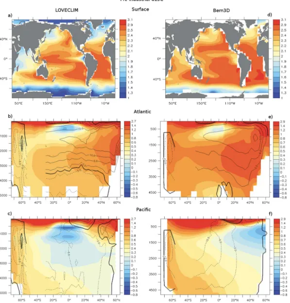
Figure 2. Preindustrial𝛿13C distribution as simulated by (a–c) LOVECLIM and the (d–f ) Bern3D model. Surface𝛿13C (‰) is shown in Figures 2a and 2b, zonally averaged𝛿13C (‰) over the Atlantic basin is shown in Figures 2c and 2d, and over the Pacific basin is shown in Figures 2e and 2f. The meridional overturning stream function (Sv) over the Atlantic basin (Figures 2c and 2d) and the Indo-Pacific basin are overlaid (Figures 2e and 2f ) north of 30∘S, and the globally integrated meridional overturning stream function (Sv) is shown over the Southern Ocean.

changes.𝛿13_{C is defined as}((13C∕12C)Sample

(13_C∕12_C) Ref)

− 1)∗ 1000, (13_C∕12_C)

Refbeing the Vienna Peedee belemnite carbon

isotope standard (0.0112372) [Craig, 1957].

At depth, remineralization of organic matter (Corg) and dissolution of calcium carbonate (CCaCO3) as well as the

preformed carbon (CPref) contribute to the DIC pool of12C and13C, so that 12_{C =}12_C

org+12CCaCO3+

12_C

Pref and 13C =13Corg+13CCaCO3+

13_C Pref. (1) Therefore, 𝛿13_{C =} 1 12_C. ( 𝛿13_C

org∗12Corg+𝛿13CCaCO3∗

12_C CaCO3+𝛿 13_C Pref∗12CPref ) . (2) Since here𝛿13_C

CaCO3∼0, we can approximate

𝛿13_{C =} 1 12_C.

(

𝛿13_C

org∗12Corg+𝛿13CPref∗12CPref

)

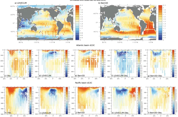
Figure 3. Present-day (years 1990–2000 A.D.)_𝛿13_{C distribution (‰) as simulated in LOVECLIM and the Bern3D model and compared to observations [Schmittner}

et al., 2013]. Ocean surface𝛿13_{C as simulated (shaded) in (a) LOVECLIM and (b) the Bern3D and compared to observations (color squared).𝛿}13_{C zonally averaged}

over the Atlantic basin and the Pacific basin only taking into account the observation locations are shown in Figures 3c–3g and 3h–3l, respectively. (c and h)𝛿13_C

from observations, (d and i) the𝛿13_{C LOVECLIM distributions, (e and j)𝛿}13_{C Bern3D distributions, (f and k) the difference between LOVECLIM and the}

observations, and (g and l) the difference between the Bern3D model and the observations. The correlation coefficients (R) between LOVECLIM (the Bern3D model) and the observations at the surface, in the Atlantic, and Pacific basins are 0.46 (0.51), 0.76 (0.74), and 0.65 (0.93), respectively.

Organic matter is depleted in13_{C (𝛿}13_C

org∼ −20‰), so that remineralization has a significant impact on

oceanic𝛿13_{C. We can estimate the effect of organic matter remineralization in the ocean in the following way:}

𝛿13_C BIO= 𝛿13_C org∗12Corg 12_C = 𝛿13_C org∗ Rc/p∗ PRem 12_C (4)

with R_c/p the carbon over phosphate Redfield ratio (117) and P_Rem the phosphate generated through remineralization. In the simulations performed with LOVECLIM, preformed phosphate (PPref) is a tracer, so

PRem= PTot− PPref. In the Bern3D, remineralized phosphate is estimated from the Apparent Oxygen Utilization

(AOU): P_Rem=AOU/R_o/p, with R_o/pthe oxygen over phosphate Redfield ratio (170). Δ𝛿13_C

THreflects the changes in𝛿13C due to air-sea gas exchange and temperature and is estimated by

Δ𝛿13_C

TH= Δ𝛿13C−Δ𝛿13CBIO.

3. Results

3.1. Preindustrial and Present-Day𝜹13_{C Distributions and Validation Against Observations}

The𝛿13_{C distribution in the ocean is governed by air-sea gas exchange, photosynthesis in the Sun-lit}

sur-face layer, export of organic matter from the sursur-face to the deep ocean, remineralization of organic matter in the deep and ocean circulation (Figure 1). On global average, DIC is isotopically enriched in the surface

Figure 4. (top to bottom) Time series of NADW, NPDW,|AABW|(Sv), as well as pCO₂(ppmv) and atmospheric𝛿13CO₂ (‰) anomalies for experiments performed with (left) LOVECLIM and (right) the Bern3D model. NADW and NPDW represent the maximum overturning stream function in the North Atlantic and the North Pacific, respectively. AABW is taken as the minimum of the global overturning stream function in the 80∘S–60∘S region and its absolute value is shown. Experiments performed with both models and with weakened NADW (Love-NA-W and Bern-NA-W) are in cyan, NADW cessation (Love-NA-Off and Bern-NA-Off ) are in blue, weakened AABW (Love-SO-W and Bern-SO-W) are in green, and strengthened AABW (Love-SO-S and Bern-SO-S) are in red. Experiments performed with LOVECLIM only: weaker (Love-SHW-W, magenta) and stronger (Love-SHW-S, black) Southern Hemispheric westerlies as well as experiments in which the CO₂air-sea gas exchange is not impacted by the wind stress changes (Love-SHW-Snas, dashed black and Love-SHW-Wnas, dashed magenta).

ocean and depleted in the deep ocean. This vertical𝛿13_{C gradient is established by the preferential uptake}

of12_{C during photosynthesis, leaving behind isotopically enriched DIC, and the export and subsequent}

rem-ineralization in the deep of isotopically depleted organic matter. Physical transport (advection, diffusion, and convection) tends to remove this vertical gradient by bringing isotopically depleted deep water to the surface and vice-versa.

The role of air-sea exchange in shaping the𝛿13_{C distribution is latitude dependent (Figure 1, inset). The}

equi-librium fraction factor increases with decreasing ocean surface temperature (∼−0.12‰/∘C) [Mook et al., 1974;

Charles et al., 1993]. As a consequence, the𝛿13_{C isotopic equilibrium with the atmosphere is higher for cold}

Figure 5.𝛿13C anomalies (‰) compared to the control run, averaged over the (a and c) Atlantic and (b and d) Pacific basin resulting from (a and b) a weakened and (c and d) a cessation of NADW formation for experiments performed with LOVECLIM (Figures 5a and 5c) and the Bern3D model (Figures 5b and 5d). The meridional overturning stream function (Sv) is overlaid for each experiment.

high-latitude surface oceans in13_{C, thereby partly mitigating the low𝛿}13_{C due to upwelling of}13_C-depleted

deep waters. At low latitudes, photosynthesis and organic matter export enrich surface water in13_{C, whereas}

air-sea exchange tends to deplete the surface ocean. Overall, this interplay results in relatively small latitudi-nal gradients in surface ocean𝛿13_{C, with slightly lower than average values in the Southern Ocean (Figure 1,}

blue lines in inset).

The preindustrial𝛿13_{C distribution as simulated in LOVECLIM and the Bern3D model is shown in Figure 2.}

In Figure 3, the simulated oceanic𝛿13_{C obtained for years 1990–2000 A.D. in the present-day experiments}

performed with LOVECLIM and the Bern3D is compared to the present-day oceanic𝛿13_{C observations}

com-piled by Schmittner et al. [2013]. Observations are from World Ocean Circulation Experiment/GLobal Ocean Data Analysis Project cruises performed in the 1990s, and thus, each observation point represents a day in time, whereas model values are averaged over a 10 year period. Both preindustrial and modern atmospheric

𝛿13_CO

2are ∼0.1‰ higher in the Bern3D model than in LOVECLIM, thus leading to globally higher oceanic

𝛿13_{C values in the Bern3D model.}

Combustion of13_{C-depleted fossil fuel since the industrial revolution increased the atmospheric CO}

2content

while decreasing atmospheric𝛿13_CO

2[Keeling, 1979; Keeling et al., 2001]. This𝛿13CO2decrease led to oceanic

𝛿13_{C decrease from preindustrial to present, particularly in the subtropical gyres. The simulated present-day}

𝛿13_{C distribution at the surface of the ocean is in general agreement with observations (Figures 3a and 3b).}

Surface𝛿13_{C is generally high at low latitude and midlatitude and low at high latitudes. The highest𝛿}13_C

values are found in the Equatorial Pacific and Atlantic, as well as the South Pacific and South Atlantic subtropical gyres.

Sustained primary production in the low-latitude upwelling zones and the subsequent advection of high𝛿13_C

waters, as well as surface ocean13_{C enrichment due to CO}

2outgassing [Lynch-Stieglitz et al., 1995] explain a

large part of the surface𝛿13_{C distribution between 40∘S and 40∘N (not shown). On the other hand, upwelling}

of low-𝛿13_{C waters and low-nutrient utilization leads to relatively low surface𝛿}13_{C in the Eastern Equatorial}

Pacific and to some extent in the Eastern Equatorial Atlantic. South of the polar front in the Southern Ocean, upwelling of low-𝛿13_{C waters, low-nutrient utilization, and invasion of depleted atmospheric CO}

2lead to the

lowest surface𝛿13_{C signature.}

Both LOVECLIM and the Bern3D model correctly simulate the𝛿13_{C signature of the main water masses}

Figure 6. Vertical𝛿13C profile anomalies averaged over (a and d) the Atlantic basin north of 20∘S, (b and e) the Southern Ocean, and (c and f ) the Pacific basin north of 20∘S for the control runs (black), NADW cessation (Love-NA-Off and Bern-NA-Off, blue), and strengthened AABW (Love-SO-S and Bern-SO-S, red).

and the lowest in the North Pacific. This gradual decrease in oceanic𝛿13_{C from the deep Atlantic to Pacific is}

due to remineralization of13_{C-depleted organic carbon. As seen in Figure 2, nutrient-depleted NADW displays}

a relatively high𝛿13_{C (0.8–1.1‰), while nutrient-rich AABW is characterized by a low𝛿}13_{C (0.4–0.6‰). The}

oldest, nutrient-rich waters lie in the deep North Pacific region and at intermediate depth in the Equatorial regions, which feature very low𝛿13_{C. In outcropping regions, air-sea gas exchange compensates for the}

low-𝛿13_{C signal brought about by organic matter remineralization, particularly associated with the AABW and}

AAIW pathways.

LOVECLIM underestimates𝛿13_{C values by an average of 0.2‰ in the Atlantic basin, while it overestimates𝛿}13_C

values by up to 0.6‰ in the intermediate North Pacific. As is also seen in its salinity structure [Menviel, 2008], the weak halocline in the North Pacific leads to an overestimated transport of high surface North Pacific

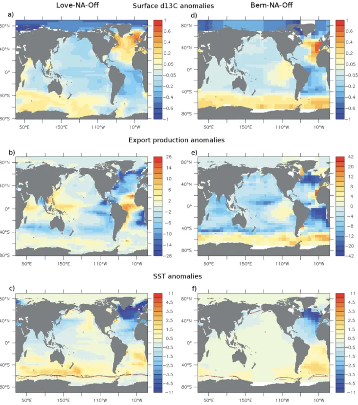
Figure 7. Results of experiments featuring a cessation of NADW formation performed with (a–c) LOVECLIM (Love-NA-Off ) and (d–f ) the Bern3D model

(Bern-NA-Off ). Surface_𝛿13_{C anomalies (‰) compared to the preindustrial control run (Figures 7a and 7d); export production anomalies (gC/m}2_{/yr) (Figures 7b}

and 7e); and SST anomalies (∘C) with the 0.1 m sea ice level overlaid for the control pre-industrial run (black) and for Love-NA-Off or Bern-NA-Off (red) (Figures 7c and 7f ).

Figure 8.𝛿13C anomalies (‰) compared to the control preindustrial run, averaged over the Atlantic (left) and Pacific basin (right) for (a–c) Love-SO-S and (d–f ) Bern-SO-S.Δ𝛿13C (‰) (Figures 8a and 8d),Δ𝛿13C_BIO(Figures 8b and 8e), andΔ𝛿13C_THFigures 8c and 8f.

associated with negative𝛿13_{C and dissolved oxygen anomalies and positive AOU anomalies when compared}

to observations [Menviel, 2008]. Weak Antarctic Intermediate Water (AAIW) formation, brought about by rela-tively weak Southern Hemispheric westerlies [Menviel, 2008], could explain the negative𝛿13_{C anomalies}

simu-lated at intermediate depth in both the South Atlantic and South Pacific. In contrast, in the Bern3D model, the North Pacific𝛿13_{C distribution is very well represented (Figures 3j and 3l), but AABW has a relatively high𝛿}13_C

signature (Figures 2 and 3).

3.2. Weakened North Atlantic Deep Water and Enhanced North Pacific Deep Water Formation

A 50% weakening (Love-NA-W and Bern-NA-W, cyan lines in Figure 4) and ∼500 m shallowing of NADW leads to positive𝛿13_{C anomalies in the upper 2000 m of the North Atlantic, with a mean anomaly of 0.09‰ over the}

region 10∘N–60∘N (Figures 5a and 5b). These positive𝛿13_{C anomalies are partly due to the reduced export}

production at the surface of the North Atlantic (−16% and −34% in Love-NA-W and Bern-NA-W, respec-tively), which reduces the remineralized carbon in the intermediate North Atlantic (Figures S1b and S1e in the supporting information). In addition, in Love-NA-W, cooler conditions in that region further enhance the sur-face𝛿13_{C increase, which is then advected to intermediate depth (Figure S1c). Conversely,𝛿}13_{C decreases by}

0.09‰ in the deep Atlantic due to increased remineralized carbon (Figures S1b and S1e), thus leading to a greater vertical𝛿13_{C gradient in the North Atlantic.}

Cessation of NADW formation (Love-NA-Off and Bern-NA-Off ) leads to negative𝛿13_{C anomalies over most of}

the Atlantic basin (Figures 5c and 5d).𝛿13_{C is about 1‰ lower at intermediate depth in the Northern North}

Atlantic as well as 0.4‰ and 0.2‰ lower in the deep North and South Atlantic, respectively.

Reduced ventilation of the deep/intermediate Atlantic leads to the accumulation of remineralized carbon, which decreases𝛿13_C

DIC. An increase in remineralized carbon in the deep and intermediate Atlantic is thus

the primary cause of the negative𝛿13_{C anomalies simulated in the Atlantic basin (Figure S2). In both models,}

NADW cessation leads to a greater vertical𝛿13_{C gradient in the Atlantic basin (Figures 6a and 6d, blue lines).}

NADW cessation is associated with weakened Northern Hemispheric poleward heat transport and thus neg-ative SST anomalies in the North Atlantic (Figures 7c and 7f ). Following the equilibrium relationship between SST changes and surface𝛿13_{C [Mook et al., 1974], a 4∘C surface cooling would lead to a𝛿}13_{C increase of 0.5‰}

Figure 9. Processes influencing atmospheric𝛿13CO₂and Southern Ocean surface𝛿13C_DICwhen AABW is enhanced (from left to right): (i) Enhanced surface-to-deep exchange brings nutrient-rich13C-depleted waters to the surface, shortens the residence time of waters in the Sun-lit surface layer, and reduces the magnitude of nutrient utilization by the marine biota. This lowers the oceanic vertical𝛿13C gradient, surface ocean𝛿13C, and atmospheric𝛿13CO2.

(ii) Reduced sea ice cover enhances air-sea gas exchange and the net transfer of13C from the atmosphere to the surface of the Southern Ocean (see Figure 1), which decreases the_𝛿13_{C disequilibrium by increasing surface ocean𝛿}13_{C and}

decreasing atmospheric_𝛿13_CO

2. (iii) Increased SST reduces the fractionation between atmospheric CO2and surface

ocean DIC, thus reducing the net transfer of13_{C from the atmosphere to the Southern Ocean, thereby lowering surface}

ocean_𝛿13_{C and increasing atmospheric𝛿}13_CO

2. (iv) Lower wind speeds associated with weaker westerlies reduce gas

transfer rates and the net13_{C gas transfer in the Southern Ocean, thereby decreasing Southern Ocean surface𝛿}13_{C and}

increasing atmospheric𝛿13_CO

2. It is the combination of these effects which ultimately determines the magnitude of the

atmospheric𝛿13_CO 2change.

at equilibrium. The equilibrium is rarely reached, particularly under sea ice (Figure S3). Enhanced nutrient uti-lization also contributes to the positive surface𝛿13_{C anomaly simulated in the North Atlantic in both models}

(Figures 7 and S3). In the Southern Ocean during NADW cessation, enhanced export production and nutri-ent utilization induce significant positive surface𝛿13_{C anomalies (Figures 7b, 7e, S3e, and S3f ), which are only}

partly compensated by the warmer surface conditions in that region. These positive𝛿13_{C anomalies spread}

from the Southern Ocean northward at intermediate depth in the AAIW core and to a smaller extent in the AABW core (Figures 5c, 5d, 6b, and 6e).

These results are broadly consistent with results from idealized meltwater experiments in which NADW formation was shut down [Marchal et al., 1998]. These authors also find negative anomalies in the deep North Atlantic and positive anomalies in the Southern Ocean related to the biological cycle and air-sea gas exchange, respectively. In contrast to LOVECLIM and the Bern3D model, the zonally averaged model used by Marchal

et al. [1998] simulates positive anomalies also in the deep Southern Ocean, probably due to extensive vertical

convection and mixing.

In LOVECLIM, strongly reduced NADW leads to the formation of North Pacific Deep Water (NPDW) through oceanic and atmospheric teleconnections [Menviel et al., 2011]. In experiment Love-NA-Off, the maximum NPDW transport is about 10 Sv at 1000 m, and NPDW reaches ∼2500 m depth (Figure 5c). NPDW is associated with a positive𝛿13_{C anomaly of up to 1‰ centered at 1500 m in the North Pacific (Figures 5c and 6c), which}

decreases southward.

Enhanced ventilation of North Pacific intermediate/deep waters reduces the release of isotopically light car-bon through remineralization and leads to positive𝛿13_{C anomalies there (Figure S2a). The formation of NPDW}

leads to the downwelling of nutrient-poor, high𝛿13_{C waters. Young, nutrient-poor, high𝛿}13_{C waters thus}

Figure 10.𝛿13C anomalies (‰) compared to the control run, zonally averaged over the Atlantic (left) and Pacific basin (right) resulting from (a and b) weakened and (c and d) strengthened AABW formation for experiments performed with LOVECLIM (Figures 10a, 10c, and 10e) and the Bern3D model (Figures 10b and 10d). (e) Experiment with enhanced Southern Hemispheric westerlies performed with LOVECLIM. The Indo-Pacific, global, and Atlantic meridional stream functions (Sv) are overlaid for each experiments.

3.3. Changes in Antarctic Bottom and Intermediate Waters

AABW strengthening either through changes in buoyancy forcing (Love-SO-S, Bern-SO-S) or increased Southern Hemispheric westerlies (Love-SHW-S) enhances the ventilation of the deep Atlantic and Pacific Oceans. The accumulation of isotopically depleted carbon originating from organic matter remineralization is reduced, which leads to positive𝛿13_C

BIOanomalies in the deep Atlantic and Pacific (Figures 8b and 8e).

Enhanced ventilation of the deep ocean leads to the upwelling of low𝛿13_{Cwaters, which decreases surface}

waters𝛿13_{C(Figures 8 and 9) as well as the vertical𝛿}13_{Cgradients (Figure 6, red).}

In addition, previous studies have shown that stronger AABW enhances the poleward heat transport to high southern latitudes [Talley, 1999], which leads to positive SST anomalies at the surface of the Southern Ocean [Menviel et al., 2015]. This SST increase lowers𝛿13_{Cat the surface of the Southern Ocean (Figure 9). The imprint}

of this signal is visible by particularly large negative𝛿13_C

THanomalies in the Southern Ocean in LOVECLIM

(Figure 8c).

Experiments Love-SO-S and Love-SHW-S display similar changes in AABW and NADW (Figure 4, red and black), and thus simulated oceanic𝛿13_{C anomalies are alike (Figure 10). However, stronger Southern Hemispheric}

westerlies also enhance the formation of AAIW, which leads to positive𝛿13_{C anomalies in the AAIW path, in}

contrast to experiment Love-SO-S.

Weaker AABW reduces the ventilation rates of the deep Pacific and Atlantic Oceans with increased accumula-tion of remineralized carbon. Negative𝛿13_{C anomalies are thus simulated in both the deep Pacific and Atlantic}

(Figures 10a and 10b). The impact of weaker AABW on oceanic𝛿13_{Csimulated in LOVECLIM and the Bern3D}

model is also in qualitative agreement with the results obtained by Kwon et al. [2012].

3.4. Relationship Between Changes in Oceanic Circulation and Atmospheric𝜹13_CO 2

Figure 4 shows the changes in atmospheric𝛿13_CO

2obtained in the different idealized experiments. NADW

cessation leads to a maximum of 0.05‰ 𝛿13_CO

2 increase, while weakened AABW transport induces a

maximum of 0.15‰𝛿13_CO

Figure 11. Scatterplot of changes in𝛿13CO₂(‰, filled) obtained with a multiple linear regression and changes in AABW, NPDW, and NADW (Sv). (a and b) Different angles of the scatterplots. The regression is performed on all the LOVECLIM experiments and is of the form:Δ𝛿13CO₂=−0.0041*ΔAABW−0.0056* ΔNPDW−0.003*ΔNADW,R2= 0.45. Triangles represent the𝛿13CO₂changes obtained at equilibrium. At equilibrium, the multiple linear regression is Δ𝛿13CO2=−0.0069*ΔAABW−0.0042*ΔNPDW−0.0012*ΔNADW,R2= 0.70. Positive (negative)ΔAABW values indicate stronger (weaker) AABW.

To get a clearer picture of the role of each water mass in controlling atmospheric𝛿13_CO

2, we perform a

multiple linear regression analysis between changes in atmospheric𝛿13_CO

2and changes in NADW, AABW,

and NPDW formation rates for the LOVECLIM experiments (Love-NA-Off, Love-NA-W, Love-SO-S, Love-SO-W, Love-SHW-Snas, and Love-SHW-Wnas). As seen in Figure 11, we find significant negative correlations between Δ𝛿13CO₂and each of the water masses transport rate (R2 _{= 0.70). Enhanced transport of AABW, NPDW, or}

NADW is thus associated with lower atmospheric𝛿13_CO

2. Standardized regression coefficients (𝛽) are −0.6894,

−0.4415, and −0.3986 for, respectively, AABW, NADW, and NPDW. This indicates that AABW ventilation rates are dominant in controlling𝛿13_CO

2variations in LOVECLIM.

Deep and intermediate water masses have a lower𝛿13_{C signature than surface waters; therefore, increased}

ventilation decreases the vertical𝛿13_{C gradient (Figure 6) by bringing low𝛿}13_{C waters to the surface and high}

𝛿13_{C waters to depth. At the same time, enhanced deep ocean ventilation lowers the accumulation of}

rem-ineralized carbon in the deep ocean (Figure 8). Enhanced AABW and NPDW formation therefore increases atmospheric CO2 [Menviel et al., 2014a], decreases surface𝛿13C, and thus𝛿13CO2(Figure 4). This result is

confirmed by a multiple linear regression analysis performed on the Bern3D experiments, which displays a significant negative correlation (R2_{= 0.6) between changes in 𝛿}13_CO

2and AABW (𝛽 = −0.97). This is also in

agreement with previous studies which found a significant impact of AABW changes on𝛿13_CO

2[Tschumi et al.,

2011; Kwon et al., 2012]. As seen in Figure 4,𝛿13_CO

2anomalies simulated in experiment Love-SHW-S and Love-SHW-W are larger

than those simulated in Love-SO-S and Love-SO-W, respectively. These differences are due to the air-sea gas exchange of13_{C and to changes in AAIW transport. Enhanced air-sea gas exchange increases the net transfer}

of13_{C from the atmosphere to the surface of the Southern Ocean (Figure 1), which increases surface ocean}

𝛿13_{C and decreases atmospheric𝛿}13_CO

2by 0.06‰ in Love-SHW-S compared to Love-SHW-Snas (Figure 4, solid

and dashed black). The reverse is true for experiment Love-SHW-W, in which reduced air-sea gas exchange increases𝛿13_CO

2by 0.06‰ compared to Love-SHW-Wnas (Figure 4, solid and dashed magenta). In addition,

stronger Southern Hemispheric westerlies strengthen AAIW, which enhances the ventilation of very low inter-mediate𝛿13_{C waters. This means that for similar changes in AABW,𝛿}13_CO

2anomalies are larger when changes

are due to dynamic forcing. This result should however be taken with caution, as AAIW𝛿13_{C signature is too}

Our results are quantitatively different from the ones obtained with the UVic ESCM [Schmittner and Lund, 2015], where a 0.25‰𝛿13_CO

2decrease is simulated following a shutdown of NADW formation over 3000 years

in an idealized North Atlantic meltwater experiment performed with interactive land biosphere. The simu-lated𝛿13_{C anomalies in their experiment are consistent with our results for a cessation of NADW formation}

coupled with formation of NPDW and/or stronger AABW formation. While enhanced NPDW and AABW formation could provide a potential explanation for the simulated decrease in atmospheric𝛿13_CO

2, the results

obtained with the UVic ESCM, LOVECLIM, and the Bern3D also seem to indicate different model sensitivities to changes in oceanic circulation.

In general, enhanced deep ocean ventilation reduces the vertical𝛿13_{C gradient and leads to atmospheric}

𝛿13_CO

2decrease. However, changing oceanic circulation also impacts the climate and the oceanic carbon

cycle. The magnitude of the atmospheric𝛿13_CO

2 change will thus also depend on additional processes.

For example, in LOVECLIM, stronger AABW (Love-SO-S) leads to a ∼1.6∘C SST increase over the Southern Ocean [Menviel et al., 2015], which reduces air-sea equilibrium fractionation, thus decreasing surface ocean

𝛿13_{C, while increasing atmospheric𝛿}13_CO

2(Figure 9). This provides a negative effect on the𝛿13CO2decrease

brought about by enhanced deep ocean ventilation. By contrast, in the Bern3D model, SST over the Southern Ocean only increase by ∼0.5∘C when AABW is enhanced (Bern-SO-S). In addition, due to the weak halocline in the North Pacific in LOVECLIM, the lower atmospheric𝛿13_CO

2leads to a𝛿13C decrease at intermediate depth

in the Pacific (Figure 8a), which buffers the atmospheric𝛿13_CO

2decrease. The different strength of these

negative effects in both models can explain the different sensitivity to changes in AABW and also in other water masses.

4. Conclusions

Here we set out to understand the impact of changes in oceanic circulation on atmospheric𝛿13_CO 2. The

main oceanic processes that can lead to an atmospheric𝛿13_CO

2decrease are higher equilibrium fractionation

during air-sea gas exchange, enhanced air-sea gas exchange, and lower surface ocean𝛿13_{C (Figure 9).}

Higher equilibrium fractionation is obtained by a cooling of sea surface waters, while enhanced air-sea gas exchange occurs in the case of stronger surface winds or reduced sea ice coverage. Lower surface ocean𝛿13_C

results from a weaker oceanic𝛿13_{C vertical gradient obtained either through weaker nutrient utilization or}

stronger ocean ventilation (Figure 9).

To a first order approximation, enhanced formation of deep and bottom waters increases the ventilation of low13_{C waters to the surface, which reduces atmospheric𝛿}13_CO

2. However, enhanced deep ocean

circula-tion is often associated with higher surface ocean temperature which tends to increase atmospheric𝛿13_CO 2

(Figure 9). Different model sensitivities with respect to changes in deep ocean circulation as well as modifica-tions of background climate condimodifica-tions will thus exert a strong constraint on the magnitude of the simulated

𝛿13_CO 2.

Analyses made on Antarctic ice cores suggest that atmospheric𝛿13_CO

2dropped by ∼0.3‰ during Heinrich

stadial 1 (HS1) [Lourantou et al., 2010; Schmitt et al., 2012], probably coincident with cessation of NADW forma-tion [McManus et al., 2004]. In contrast with a previous study [Schmittner and Lund, 2015], our results suggest that a cessation of NADW formation has little impact on atmospheric𝛿13_CO

2and thus cannot explain the

measured𝛿13_CO

2decrease. Paleoproxy records have suggested that Southern Ocean ventilation was stronger

during HS1 [e.g., Anderson et al., 2009; Skinner et al., 2010], and previous modeling studies have shown that enhanced AABW during HS1 would increase atmospheric CO2[Menviel et al., 2014a] and decrease atmospheric

Δ14C [Matsumoto and Yokoyama, 2013] in agreement with paleorecords. In addition, Tschumi et al. [2011] find in their model that enhanced Southern Ocean ventilation decreases atmospheric𝛿13_CO

2, and Southern Ocean

surface d13C, while increasing deep ocean𝛿13_{C, Δ}13_{C and oxygen. In addition, Southern Ocean opal export}

and opal sediment burial increase, initially deepening the lysocline, all consistent with proxy information [e.g., Broecker and Clark, 2001; Anderson et al., 2009; Schmitt et al., 2012; Jaccard et al., 2014].

AABW could have been enhanced during HS1 either through buoyancy forcing or through stronger/poleward shifted Southern Hemispheric westerlies. For example, a reduced temperature gradient in the Southern Hemisphere as well as a southward shift of the Intertropical Convergence Zone in response to weakened NADW formation could enhance and shift the Southern Hemispheric westerlies poleward [Toggweiler et al., 2006; Denton et al., 2010; Toggweiler and Lea, 2010; Lee et al., 2011]. Stronger Southern Hemispheric westerlies

during HS1 would enhance AABW and AAIW, as well as the air-sea CO2exchange. Here we simulate a 0.15‰

reduction in atmospheric𝛿13_CO

2when increasing the Southern Hemispheric westerlies by 35%. In addition,

reduced iron fertilization at the beginning of the deglaciation would diminish nutrient utilization over the Southern Ocean, which would further decrease atmospheric𝛿13_CO

2by 0.1 to 0.2‰ [Lourantou et al., 2010;

Menviel et al., 2012; Broecker and McGee, 2013]. Our results thus suggest that enhanced AABW during HS1

combined with reduced iron fertilization could explain the 0.3‰ 𝛿13_CO

2 decrease. Further studies are

needed to investigate the impact of boundary conditions on changes in atmospheric𝛿13_CO

2and verify this

hypothesis.

Appendix A

Temperature dependent fractionation occurs during the air-sea gas exchange of CO2as well as the

dissocia-tion of aqueous CO2into bicarbonate (HCO−3) and carbonate (CO 2−

3 ) ions. Due to the long timescale required

for the oceanic surface to be in equilibrium with the atmosphere, water mass formation, sea ice cover, and mixing also have an impact on oceanic𝛿13_C.

The kinetic fractionation factor during air-sea gas exchange has a weak dependence on temperature (T, ∘K) [Siegenthaler and Münnich, 1981]:

𝛼K= 0.9995 ∗ (1.00019 − 0.373∕T) (A1) During photosynthesis,12_{C is preferentially taken up, so that organic matter is depleted in}13_{C. Freeman}

and Hayes [1992] defined the isotopic difference between dissolved CO2(𝛿13Cd) and primary photosynthate

(𝛿13_C om) as 𝜖d−om= ( (𝛿13_C d+ 1000) (𝛿13_C om+ 1000) − 1 ) ∗ 1000 ∼𝛿13Cd−𝛿13Com (A2)

In this study,𝜖d−omis set constant at 22‰ in LOVECLIM.

References

Anderson, R. F., S. Ali, L. I. Bradtmiller, S. H. H. Nielsen, M. Q. Fleisher, B. E. Anderson, and L. H. Burckle (2009), Wind-driven upwelling in the Southern Ocean and the deglacial rise in Atmospheric CO₂, Science, 323, 1443–1448.

Bouttes, N., D. Paillard, D. M. Roche, V. Brovkin, and L. Bopp (2011), Last Glacial Maximum CO₂and𝛿13C successfully reconciled, Geophys. Res. Lett., 38, L02705, doi:10.1029/2010GL044499.

Broecker, W. S. (1997), Thermohaline circulation, the Achilles heel of our climate system: Will man-made CO₂upset the current balance?, Science, 278, 1582–1588.

Broecker, W. S. (1998), Paleocean circulation during the last deglaciation: A bipolar seesaw?, Paleoceanography, 13, 119–121. Broecker, W. S., and E. Clark (2001), Redistribution of carbonate ion in the deep sea, Science, 294, 2152–2155.

Broecker, W. S., and D. McGee (2013), The13C record for atmospheric CO₂: What is it trying to tell us?, Earth Planet. Sci. Lett., 368, 175–182. Brovkin, V., A. Ganopolski, and Y. Svirezhev (1997), A continuous climate-vegetation classification for use in climate-biosphere studies,

Ecol. Modell., 101, 251–261.

Brovkin, V., J. Bendtsen, M. Claussen, A. Ganopolski, C. Kubatzki, V. Petoukhov, and A. Andreev (2002), Carbon cycle, vegetation, and climate dynamics in the Holocene: Experiments with the CLIMBER-2 model, Global Biogeochem. Cycles, 4, 1139, doi:10.1029/2001GB001662. Brovkin, V., A. Ganopolski, D. Archer, and S. Rahmstorf (2007), Lowering of glacial atmospheric CO2in response to changes in oceanic

circulation and marine biogeochemistry, Paleoceanography, 22, PA4202, doi:10.1029/2006PA001380.

Burke, A., and L. F. Robinson (2012), The Southern Ocean’s role in carbon exchange during the last deglaciation, Science, 335, 557–561. Charles, C. D., J. D. Wright, and R. G. Fairbanks (1993), Thermodynamics influences on the marine carbon isotope record, Paleoceanography,

8, 691–697.

Craig, H. (1957), Isotopic standards for carbon and oxygen and correction factors for mass-spectrometric analysis of carbon dioxide, Geochim. Cosmochim. Acta, 12, 133–149.

Denton, G. F., R. F. Anderson, J. R. Toggweiler, R. L. Edwards, J. M. Schaefer, and A. E. Putnam (2010), The last glacial termination, Science, 328, 1652–1656.

Elsig, J., J. Schmitt, D. Leuenberger, R. Schneider, M. Eyer, M. Leuenberger, F. Joos, H. Fischer, and T. F. Stocker (2009), Stable isotope constraints on Holocene carbon cycle changes from an Antarctic ice core, Nature, 461, 507–510.

Fichefet, T., M.-F. Loutre, P. Huybrechts, H. Goelzer, and A. Mouchet (2012), Assessment of modelling uncertainties in long-term climate and sea level change projections “ASTER”, Final Rep., BELSPO. Bruxelles, Belgium.

Francey, R. J., C. E. Allison, D. M. Etheridge, C. M. Trudinger, I. G. Enting, M. Leuenberger, R. L. Langenfelds, E. Michel, and L. P. Steele (1999), A 1000-year high precision record of𝛿13C in atmospheric CO₂, Tellus B, 51, 170–193.

Freeman, K. H., and J. M. Hayes (1992), Fractionation of carbon isotopes by phytoplankton and estimates of ancient CO₂levels, Global Biogeochem. Cycles, 6, 185–198.

Galbraith, E. D., E. Y. Kwon, D. Bianchi, M. P. Hain, and J. L. Sarmiento (2015), The impact of atmospheric pCO2 on carbon isotope ratios of the atmosphere and ocean, Global Biogeochem. Cycles, 29, 307–324, doi:10.1002/2014GB004929.

Ganopolski, A., and S. Rahmstorf (2001), Rapid changes of glacial climate simulated in a coupled climate model, Nature, 409, 153–158. Acknowledgments

This project was supported by the Australian Research Council. L. Menviel and M. England acknowledge fund-ing from the Australian Research Council grants DE150100107 and FL100100214, respectively. K. Meissner acknowledges support from the UNSW Goldstar award. F.J. acknowl-edges funding by the Swiss National Science Foundation. We thank the Editor S. Mikaloff Fletcher, the Asso-ciate Editor K. Matsumoto, and R.J. Toggweiler, as well as an anony-mous reviewer for insightful com-ments. We thank Raphael Roth for per-forming the modern experiment with the Bern3D model and W.T. Hiscock for graphical design. LOVECLIM experiments were performed on a computational cluster owned by the Faculty of Science of the University of New South Wales, Sydney, Australia. Bern3D experiments were performed on a computational cluster owned by the Department of Environmen-tal Physics of the University of Bern, Switzerland. Results of the model-ing experiments are available upon request to the authors. The authors wish to acknowledge use of the Ferret program for analysis and graph-ics in this paper. Ferret is a product of NOAA’s Pacific Marine Environmental Laboratory. (Information is available at http://ferret.pmel.noaa.gov/Ferret/).

Gehlen, M., L. Bopp, N. Emprin, O. Aumont, C. Heinze, and O. Ragueneau (2006), Reconciling surface ocean productivity, export fluxes and sediment composition in a global biogeochemical ocean model, Biogeosciences, 3, 521–537.

Gerber, M., and F. Joos (2013), An ensemble Kalman filter multi-tracer assimilation: Determining uncertain ocean model parameters for improved climate-carbon cycle projections, Ocean Modell., 64, 29–45.

Goosse, H., et al. (2010), Description of the Earth system model of intermediate complexity LOVECLIM version 1.2, Geosci. Model Dev., 3, 603–633.

Heinrich, H. (1988), Origin and consequences of cyclic ice rafting in the northeast Atlantic Ocean during the past 130,000 years, Quat. Res., 29, 142–152.

Heinze, C., E. Maier-Reimer, A. M. E. Winguth, and D. Archer (1999), A global oceanic sediment model for long-term climate studies, Global Biogeochem. Cycles, 13, 221–250.

Hoefs, J. (1997), Stable Isotope Geochemistry, 4th ed., Springer, Berlin.

Indermühle, A., et al. (1999), Holocene carbon cycle dynamics based on CO₂trapped in ice at Taylor Dome, Antarctica, Nature, 398, 121–126.

Jaccard, S. L., E. D. Galbraith, T. L. Froelicher, and N. Gruber (2014), Ocean (de)oxygenation across the last deglaciation: Insights for the future, Oceanography, 27, 26–35.

Joos, F., S. Gerber, I. C. Prentice, B. L. Otto-Bliesner, and P. J. Valdes (2004), Transient simulations of Holocene atmospheric carbon dioxide and terrestrial carbon since the Last Glacial Maximum, Global Biogeochem. Cycles, 18, GB2002, doi:10.1029/2003GB002156. Kalnay, E., et al. (1996), The NCEP/NCAR 40-year reanalysis project, Bull. Am. Meteorol. Soc., 77, 437–471.

Keeling, C. D. (1979), The Suess effect:13carbon-14carbon interrelations, Environ. Int., 2, 229–300.

Keeling, C. D., S. C. Piper, R. B. Bacastow, M. Wahlen, T. P. Whorf, M. Heimann, and H. A. Meijer (2001), Exchanges of Atmospheric CO₂and

13_CO

2With the Terrestrial Biosphere and Oceans From 1978 to 2000. I. Global Aspects, Scripps Inst. of Oceanography, Univ. of California,

San Diego, Calif.

Köhler, P., H. Fischer, and J. Schmitt (2010), Atmospheric𝛿13CO2and its relation to pCO2and deep ocean𝛿13C during the late Pleistocene,

Paleoceanography, 25, PA1213, doi:10.1029/2008PA001703.

Krakauer, N. Y., J. T. Randerson, F. W. Primeau, N. Gruber, and D. Menemenlis (2006), Carbon isotope evidence for the latitudinal distribution and wind speed dependence of the air-sea gas transfer velocity, Tellus B, 58, 390–417.

Kwon, E. Y., M. P. Hain, D. M. Sigman, E. D. Galbraith, J. L. Sarmiento, and J. R. Toggweiler (2012), North Atlantic ventilation of “southern-sourced” deep water in the glacial ocean, Paleoceanography, 27, PA2208, doi:10.1029/2011PA002211.

Lee, S.-Y., J. C. H. Chiang, K. Matsumoto, and K. S. Tokos (2011), Southern Ocean wind response to North Atlantic cooling and the rise in atmospheric CO₂: Modeling perspective and paleoceanographic implications, Paleoceanography, 26, PA1214, doi:10.1029/2010PA002004.

Lourantou, A., J. V. Lavric, P. Kohler, J.-M. Barnola, D. Paillard, E. Michel, D. Raynaud, and J. Chappellaz (2010), Constraint of the CO₂ rise by new atmospheric carbon isotopic measurements during the last deglaciation, Global Biogeochem. Cycles, 24, GB2015, doi:10.1029/2009GB003545.

Lynch-Stieglitz, J., T. F. Stocker, W. S. Broecker, and R. G. Fairbanks (1995), The influence of air-sea exchange on the isotopic composition of oceanic carbon: Observations and modeling, Global Biogeochem. Cycles, 9, 653–665.

Marchal, O., T. F. Stocker, and F. Joos (1998), Impact of oceanic reorganizations on the ocean carbon cycle and atmospheric carbon dioxide content, Paleoceanography, 13, 225–244.

Matsumoto, K., and Y. Yokoyama (2013), AtmosphericΔ14_{C reduction in simulations of Atlantic overturning circulation shutdown, Global}

Biogeochem. Cycles, 27, 296–304, doi:10.1002/gbc.20035.

McManus, J. F., R. Francois, J. M. Gherardi, L. D. Keigwin, and S. Brown-Leger (2004), Collapse and rapid resumption of Atlantic meridional circulation linked to deglacial climate changes, Nature, 428, 834–837.

Menviel, L. (2008), Climate-carbon cycle interactions on millennial to glacial timescales as simulated by a model of intermediate com-plexity, LOVECLIM, PhD. thesis, University of Hawai’i, Honolulu, Hawaii. [Available at http://myweb.science.unsw.edu.au/lauriemenviel/ Menvielthesis2008.pdf.]

Menviel, L., and F. Joos (2012), Towards explaining the Holocene carbon dioxide and carbon isotope records: Results from transient carbon cycle-climate simulations, Paleoceanography, 27, PA1207, doi:10.1029/2011PA002224.

Menviel, L., A. Timmermann, O. Timm, and A. Mouchet (2011), Deconstructing the last glacial termination: The role of millennial and orbital-scale forcings, Quat. Sci. Rev., 30, 1155–1172.

Menviel, L., F. Joos, and S. P. Ritz (2012), Modeling atmospheric CO₂, stable carbon isotope and marine carbon cycle changes during the last glacial-interglacial cycle, Quat. Sci. Rev, 56, 46–68.

Menviel, L., M. H. England, K. J. Meissner, A. Mouchet, and J. Yu (2014a), Atlantic-Pacific seesaw and its role in outgassing CO₂during Heinrich events, Paleoceanography, 29, 58–70, doi:10.1002/2013PA002542.

Menviel, L., A. Timmermann, T. Friedrich, and M. H. England (2014b), Hindcasting the continuum of Dansgaard-Oeschger variability: Mechanisms, patterns and timing, Clim. Past, 10, 63–77, doi:10.5194/cp-10-63-2014.

Menviel, L., P. Spence, and M. H. England (2015), Contribution of enhanced Antarctic Bottom Water formation to Antarctic warm events and millennial-scale atmospheric CO₂increase, Earth Planet. Sci. Lett., 413, 37–50.

Mook, W. G. (1986),13Cin atmospheric CO₂, Neth. J. Sea Res., 20, 211–223.

Mook, W. G., J. C. Bommerson, and W. H. Staverman (1974), Carbon isotope fractionation between dissolved bicarbonate and gaseous carbon dioxide, Earth Planet. Sci. Lett., 22, 169–176.

Mouchet, A. (2011), A 3D model of ocean biogeochemical cycles and climate sensitivity studies, PhD thesis, Université de Liège, Lìege, Belgium. [Available at http://hdl.handle.net/2268/98995.]

Mouchet, A. (2013), The ocean bomb radiocarbon inventory revisited, Radiocarbon, 55, 1580–594.

Müller, S. A., F. Joos, N. R. Edwards, and T. F. Stocker (2006), Water mass distribution and ventilation time scales in a cost-efficient three-dimensional ocean model, J. Clim., 19, 5479–5499.

Müller, S. A., F. Joos, N. R. Edwards, and T. F. Stocker (2008), Modeled natural and excess radiocarbon: Sensitivities to the gas exchange formulation and ocean transport strength, Global Biogeochem. Cycles, 22, GB3011, doi:10.1029/2007GB003065.

Najjar, R. G., J. Orr, C. L. Sabine, and F. Joos (1999), Biotic-HOWTO, Internal ocmip Rep., LSCE/CEA Saclay. Gif-sur-Yvette, France.

Okazaki, Y., A. Timmermann, L. Menviel, N. Harada, A. Abe-Ouchi, M. Chikamoto, A. Mouchet, and H. Asahi (2010), Deep water formation in the North Pacific during the last glacial termination, Science, 329, 200–204.

Okumura, Y. M., C. Deser, A. Hu, A. Timmermann, and S.-P. Xie (2009), North Pacific climate response to freshwater forcing in the subarctic North Atlantic: Oceanic and atmospheric pathways, J. Clim., 22, 1424–1445.

Parekh, P., F. Joos, and S. A. Müller (2008), A modeling assessment of the interplay between aeolian iron fluxes and iron-binding ligands in controlling carbon dioxide fluctuations during Antarctic warm events, Paleoceanography, 23, PA4202, doi:10.1029/2007PA001531. Rae, J. W. B., M. Sarnthein, G. L. Foster, A. Ridgwell, P. M. Grootes, and T. Elliott (2014), Deep water formation in the North Pacific and deglacial

CO2rise, Paleoceanography, 29, 645–667, doi:10.1002/2013PA002570.

Ritz, S. P., T. F. Stocker, and F. Joos (2011), A coupled dynamical ocean—Energy balance atmosphere model for paleoclimate studies, J. Clim., 24, 349–375.

Roth, R., and F. Joos (2013), A reconstruction of radiocarbon production and total solar irradiance from the Holocene14C and CO₂records: Implications of data and model uncertainties, Clim. Past, 9, 1879–1909.

Rubino, M., et al. (2013), A revised 1000 year atmospheric𝛿13C-CO₂record from Law Dome and South Pole, Antarctica, J. Geophys. Res. Atmos., 118, 8482–8499, doi:10.1002/jgrd.50668.

Saenko, O. A., A. Schmittner, and A. J. Weaver (2004), The Atlantic-Pacific seesaw, J. Clim., 17, 2033–2038. Schmitt, J., et al. (2012), Carbon isotope constraints on the deglacial CO₂rise from ice cores, Science, 136, 711–714.

Schmittner, A., and D. C. Lund (2015), Early deglacial Atlantic overturning decline and its role in atmospheric CO2rise inferred from carbon

isotopes (𝛿13C), Clim. Past, 11, 135–152.

Schmittner, A., N. Gruber, A. C. Mix, R. M. Key, A. Tagliabue, and T. K. Westberry (2013), Biology and air-sea gas exchange controls on the distribution of carbon isotope ratios (𝛿13C) in the ocean, Biogeosciences, 10, 5793–5816.

Siegenthaler, U., and K. O. Münnich (1981),13C∕12_{C fractionation during CO}

2transfer from air to sea, in SCORE 16: Carbon Cycle Modelling,

edited by B. Bolin, pp. 249–257, Wiley, Chichester, England.

Siegenthaler, U., and H. Oeschger (1987), Biospheric CO₂emissions during the past 200 years reconstructed by convolution of ice core data, Tellus B, 39, 140–154.

Skinner, L. C., S. Fallon, C. Waelbroeck, E. Michel, and S. Barker (2010), Ventilation of the deep Southern Ocean and deglacial CO₂rise, Science, 328, 1147–1151.

Smith, H. J., H. Fischer, M. Wahlen, D. Mastroianni, and B. Deck (1999), Dual modes of the carbon cycle since the Last Glacial Maximum, Nature, 400, 248–250.

Talley, L. D. (1999), Some aspects of ocean heat transport by the shallow, intermediate and deep overturning circulations, in Mechanisms of Global Climate Change at Millennial Time Scales, Geophys. Monogr. Ser., vol. 112, edited by P. U. Clark, R. S. Webb, and L. D. Keigwin, pp. 1–22, AGU, Washington, D. C.

Toggweiler, J. R., and D. W. Lea (2010), Temperature differences between the hemispheres and ice age climate variability, Paleoceanography, 25, PA2212, doi:10.1029/2009PA001758.

Toggweiler, J. R., J. L. Russell, and S. R. Carson (2006), Midlatitude westerlies, atmospheric CO₂, and climate change during ice ages, Paleoceanography, 21, PA2005, doi:10.1029/2005PA001154.

Tschumi, T., F. Joos, and P. Parekh (2008), How important are Southern Hemisphere wind changes for low glacial carbon dioxide? A model study, Paleoceanography, 23, PA4208, doi:10.1029/2008PA001592.

Tschumi, T., F. Joos, M. Gehlen, and C. Heinze (2011), Deep ocean ventilation, carbon isotopes, marine sedimentation and the deglacial CO₂ rise, Clim. Past, 7, 771–800.

Turner, J. V. (1982), Kinetic fractionation of carbon-13 during calcium carbonate precipitation, Geochim. Cosmochim. Acta, 46, 1183–1191. Wanninkhof, R. (1992), Relationship between gas exchange and wind speed over the ocean, J. Geophys. Res., 97, 7373–7381.

Zhang, J., P. D. Quay, and D. O. Wilbur (1995), Carbon isotope fractionation during gas-water exchange and dissolution of CO₂, Geochim. Cosmochim. Acta, 59, 107–114.