HAL Id: cea-01323601
https://hal-cea.archives-ouvertes.fr/cea-01323601
Submitted on 30 May 2016
HAL is a multi-disciplinary open access
archive for the deposit and dissemination of
sci-entific research documents, whether they are
pub-lished or not. The documents may come from
teaching and research institutions in France or
abroad, or from public or private research centers.
L’archive ouverte pluridisciplinaire HAL, est
destinée au dépôt et à la diffusion de documents
scientifiques de niveau recherche, publiés ou non,
émanant des établissements d’enseignement et de
recherche français ou étrangers, des laboratoires
publics ou privés.
Characterizing flow fluctuations with moments
Rajeev S. Bhalerao, Subrata Pal, Jean-Yves Ollitrault
To cite this version:
Rajeev S. Bhalerao, Subrata Pal, Jean-Yves Ollitrault. Characterizing flow fluctuations with moments.
Physics Letters B, Elsevier, 2015, 742, pp.94-98. �10.1016/j.physletb.2015.01.019�. �cea-01323601�
arXiv:1411.5160v2 [nucl-th] 22 Jan 2015
Characterizing flow fluctuations with moments
Rajeev S. Bhalerao,1 Jean-Yves Ollitrault,2 and Subrata Pal3
1
Department of Theoretical Physics, Tata Institute of Fundamental Research, Homi Bhabha Road, Colaba, Mumbai 400 005, India
2
CNRS, URA2306, IPhT, Institut de physique th´eorique de Saclay, F-91191 Gif-sur-Yvette, France
3
Department of Nuclear and Atomic Physics, Tata Institute of Fundamental Research, Homi Bhabha Road, Mumbai, 400005, India
(Dated: January 23, 2015)
We present a complete set of multiparticle correlation observables for ultrarelativistic heavy-ion collisions. These include moments of the distribution of the anisotropic flow in a single harmonic, and also mixed moments, which contain the information on correlations between event planes of different harmonics. We explain how all these moments can be measured using just two symmetric subevents separated by a rapidity gap. This presents a multi-pronged probe of the physics of flow fluctuations. For instance, it allows to test the hypothesis that event-plane correlations are generated by non-linear hydrodynamic response. We illustrate the method with simulations of events in A MultiPhase Transport (AMPT) model.
PACS numbers: 25.75.Ld, 24.10.Nz
I. INTRODUCTION
Large anisotropic flow has been observed in ultra-relativistic nucleus-nucleus collisions at the Relativistic Heavy-Ion Collider (RHIC) and the Large Hadron Col-lider (LHC) [1]. Anisotropic flow is an azimuthal (ϕ) asymmetry of the single-particle distribution [2]:
P (ϕ) = 1 2π +∞ X n=−∞ Vne −inϕ , (1)
where Vn is the (complex) anisotropic flow coefficient in
the nth harmonic. One usually uses the notation vn for
the magnitude: vn ≡ |Vn|. Anisotropic flow is
under-stood as the hydrodynamic response to spatial deforma-tion of the initial density profile. This profile fluctuates event to event, which implies that the flow also fluctu-ates [3, 4]. The recognition of the importance of flow fluctuations has led to a wealth of new flow observables, among which triangular flow [5] and higher harmonics, as well as correlations between different Fourier harmon-ics [6].
Flow fluctuations provide a window [7] into both the early stage dynamics and the transport properties of the quark-gluon plasma. Specifically, the magnitudes of higher-order harmonics (V3 to V6) are increasingly
sen-sitive to the shear viscosity to entropy density ratio [8]. The distributions of V2 and V3 carry detailed
informa-tion about the initial density profile [9, 10], while V4 and
higher harmonics are understood as superpositions of lin-ear and nonlinlin-ear responses, through which they are cor-related with lower-order harmonics [11, 12]. Ideally, one would like to measure the full probability distribution p(V1, V2, · · · , Vn) [13]. So far, only limited information
has been obtained, concerning either the distribution of a single Vn [14] or specific angular correlations between
different harmonics [6].
We propose to study the distribution p(V1, V2, · · · , Vn)
via its moments in various harmonics [15, 16], either sin-gle or mixed, and illustrate our point with realistic sim-ulations using the AMPT model [17]. In Sec. II, we re-call how moments can be measured simply with a sin-gle rapidity gap [18]. This procedure is less demanding in terms of detector acceptance than the one based on several rapidity windows separated pairwise by gaps [6], and can be used to study even four-plane correlators. In Sec. III, we list standard measures of flow fluctua-tions which have been used in the literature and express them in terms of moments. In Sec. IV, we introduce new observables which shed additional light on the ori-gin of event-plane correlations. For instance, a corre-lation between (V2)2 and V4 has been observed, which
increases with impact parameter [6]. This correlation is usually understood [19] as an effect of the non-linear hy-drodynamic response which creates a V4 proportional to
(V2)2 [11, 20, 21]: the increase in the correlation is thus
assumed to result from the increase of elliptic flow [22]. We show that this hypothesis can be tested directly by studying how the correlation between (V2)2 and V4 is
correlated with the magnitude of V2. We also investigate
in a similar way the origin of the three-plane correlation between V2, V3 and V5 [6].
II. MEASURING MOMENTS
The statistical properties of Vn are contained in its
moments, which are average values of products of Vn, of
the form M ≡ * Y n (Vn)kn(V ∗ n)ln + , (2)
where kn and ln are integers, and angular brackets
de-note an average value over events. Note that V∗
n = V−n
2 nontrivial moments satisfy [23]
X n nkn= X n nln. (3)
We now describe a simple procedure for measuring these moments, which applies to harmonics n ≥ 2, i.e., k1 = l1 = 0. (We do not study here moments involving
directed flow V1[23].) We define in each collision the flow
vector [24] by Qn ≡ 1 N X j einϕj, (4)
where the sum runs over N particles seen in a reference detector, and ϕj are their azimuthal angles.1 One
typi-cally measures Qn in two different parts of the detector
(“subevents” [28]) A and B, which are symmetric around midrapidity and separated by a gap in pseudorapidity (i.e., polar angle) [29]. The moment (2) is then given by
M ≡ * Y n (Vn)kn(V ∗ n)ln + = * Y n (QnA)kn(Q ∗ nB)ln + , (5) which one can symmetrize over A and B to decrease the statistical error. This configuration, with all factors of Qnon one side and all factors of Q∗non the other side [18],
suppresses nonflow correlations and self correlations as long as only harmonics n ≥ 2 are involved. An alter-native procedure, where self correlations are explicitly subtracted, is described in [15].
In order to illustrate the validity of the method, we perform calculations using the AMPT model [17]. AMPT reproduces quite well LHC data for anisotropic flow (v2
to v6) at all centralities [30–32]. The implementation
adopted in this paper [33] uses initial conditions from the HIJING 2.0 model [34], which contains nontrivial event-by-event fluctuations. Flow in AMPT is produced by elastic scatterings in the partonic phase. In addition, the model contains resonance decays, and thus nontrivial nonflow effects. In the present work, subevent A consists of all particles in the pseudorapidity range 0.4 < η < 4.8, and subevent B is symmetric around mid-rapidity, so that there is an η gap of 0.8 between A and B [35].
The thumb rule for measuring moments is that smaller values of n are easier to measure because vn decreases
with n for n ≥ 2. Lower order moments, corresponding to smaller values of kn and ln, are also easier because
higher-order moments are plagued with large variances, which entail large statistical errors.
1
The factor 1/N in Eq. (4) means that we choose to average over particles in each event [25], rather than summing [24, 26] or dividing by 1/√N [27]. This choice is discussed at the end of Sec. III. 1 2 3 4 5
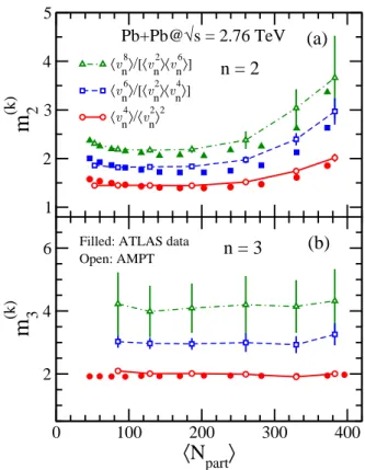
m
2 (k) 〈v n 8 〉/[〈v n 2 〉〈v n 6 〉] 〈v n 6〉 /[〈v n 2〉〈 v n 4〉 ] 〈v n 4 〉/〈v n 2 〉2 0 100 200 300 400〈
N
part〉
2 4 6m
3 (k)n = 2
n = 3
Pb+Pb@
√
s = 2.76 TeV
(a)
(b)
Filled: ATLAS data Open: AMPT
FIG. 1. (Color online) Scaled moments of the distribution of vn, (see Eq. (6)) for k = 2, 3, 4, as a function of centrality,
measured with the number of participant nucleons. Results are for (a) elliptic flow, n = 2, and (b) triangular flow, n = 3, in Pb-Pb collisions at √s = 2.76 TeV. Open symbols rep-resent AMPT calculations and closed symbols are obtained from ATLAS data [36].
III. vn FLUCTUATIONS, EVENT-PLANE
CORRELATIONS, STANDARD CANDLES We first list observables which have been previously studied in the literature and explain how they can be measured using the method outlined in Sec. II. Fluc-tuations of vn have been studied using cumulants [37–
40], which are linear combinations of even moments of the distribution of vn, that is, h(vn)2ki. These moments
are obtained by keeping only one value of n and setting kn = ln = k in Eq. (5). Figure 1 displays the scaled
moments m(k)n ≡ hv2k n i hv2(k−1)n ihvn2i , (6)
for k = 2, 3, 4 as a function of centrality for n = 2 and n = 3, obtained by using the subevent method of Sec. II. The scaled moment m(k)n thus defined is invariant if one
multiplies vnby a constant, therefore it reflects the
statis-tics of vnand should be essentially independent of the
de-tector acceptance. AMPT calculations are in fair agree-ment with the ATLAS data [36], but tend to slightly overpredict m(k)n , i.e., overestimate flow fluctuations.
0
100
200
300
400
〈
N
part〉
1
2
3
4
correlation
〈v 2 2 v 5 2〉 /[〈v 2 2〉〈 v 5 2〉 ] 〈v 3 2 v 5 2 〉/[〈v 3 2 〉〈v 5 2 〉]0
100
200
300
400
〈
N
part〉
1
2
3
4
correlation
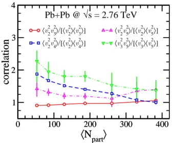
〈v 2 2 v 3 2〉 /[〈v 2 2〉〈 v 3 2〉 ] 〈v 2 2 v 4 2 〉/[〈v 2 2 〉〈v 4 2 〉]Pb+Pb @
√
s = 2.76 TeV
FIG. 2. (Color online) Correlations between v2 n and v
2 mas a
function of centrality for (n, m) = (2, 3), (2, 4), (2, 5), (3, 5), in Pb-Pb collisions at√s = 2.76 TeV calculated in the AMPT model.
If flow is solely created by fluctuations and if the statis-tics of these fluctuations is a 2-dimensional Gaussian [41], then m(k)n = k. As can be seen in Fig. 1(b), m(k)3 ≃ k for
all centralities, as expected since v3is only from
fluctua-tions in Pb-Pb collisions.2 Similarly, as seen in Fig. 1(a),
m(k)2 is roughly equal to k for central collisions where v2
is mostly from Gaussian fluctuations, but decreases for mid-central collisions, corresponding to the emergence of a mean elliptic flow in the reaction plane [43].
Event-plane correlations [6] can also be expressed in terms of moments which can be measured using the method outlined in Sec. II, as already discussed in Ref. [18]. Specifically, two-plane correlations are Pearson correlation coefficients between moments.3 The Pearson
correlation coefficient between two complex variables f and g whose average value is 0, hf i = hgi = 0, is defined as
r ≡ hf g
∗
i
ph|f|2i h|g|2i. (7)
|r| ≤ 1 in general, and r = 0 if f and g are uncorre-lated. The correlation between the second and fourth harmonic planes, which is denoted by hcos(4(Φ2− Φ4))iw
in Ref. [6], corresponds to f = V4, g = (V2)2. The largest
source of uncertainty in this measurement is the denom-inator which involves v2
4 , a measurement quadratic in
the small harmonic V4.
2
Small deviations from Gaussian statistics are actually seen ex-perimentally and result in a non-zero cumulant v3{4} [42]. Our
simulation does not have enough statistics to detect this small non-Gaussianity.
3
Three- and four-plane [44] correlations are not Pearson coeffi-cients and are not bounded by unity [25].
Note that the scaled moments Eq. (6) are of the type hf gi / hf i hgi, which is another measure of the correla-tion between f and g when hf i and hgi both differ from 0. This correlation measure equals unity if f and g are uncorrelated, and is larger than unity if there is a posi-tive correlation. It is in general easier to measure than the Pearson correlation coefficient, because it does not involve the higher-order moments|f |2 and |g|2 .
The “standard candles” introduced in Ref. [15] corre-spond to the case f = v2
n, g = v2m, obtained by keeping
only two harmonics, n and m, and setting kn = km =
ln = lm= 1 in Eq. (5). These are correlations between
the magnitudes vn and vm, which do not involve the
an-gular correlation between event planes. Four of these cor-relations are displayed in Fig. 2. The correlation between v2
2 and v23 is small and negative (hv22v23i − hv22ihv23i < 0),
as already seen in AMPT calculations [45], while the cor-relation between the corresponding event planes is small and positive [6]. All other correlations are positive. The correlation between v4 and v2, and that between v5 and
v3, become smaller for more central collisions, which is
likely due to the smaller non-linear contributions [21] of v4and v5, respectively.
Note that the observables in Eq. (6) and Eq. (7) are defined in such a way that factors of 1/N in Eq. (4) can-cel between the numerator and the denominator if N is the same for all events. In general, N fluctuates, and the result depends on whether or not one includes a factor 1/N . However, the centrality selection in experiments is typically done using the multiplicity in a reference de-tector (see e.g. Ref. [22]) so that effects of multiplicity fluctuations are likely to be small in narrow centrality intervals. The calculations in this paper are done with a 1/N normalization, but there is no strong argument for preferring one normalization over another.
IV. TESTING THE NON-LINEAR RESPONSE USING MOMENTS
We now introduce new correlation measures of the type hf gi / hf i hgi in order to study how event-plane correla-tions are correlated with the magnitude of anisotropic flow. We first consider the case f = V4(V2∗)2and g = v22.
hf gi is obtained by setting k2 = k4 = 1 and l2 = 3
in Eq. (5). The correlation hf gi / hf i hgi is displayed in Fig. 3(a). There is a significant positive correlation for all centralities, which becomes larger for central colli-sions. In hydrodynamics, the correlation between V4and
(V2)2originates from a non-linear response [19]. In order
to test this hypothesis, we model V4 as the sum of two
terms:
V4= V4l+ βV22, (8)
where the non-linear response coefficient β is the same for all events in a centrality class. This corresponds to the separation of V4into a linear part, created by
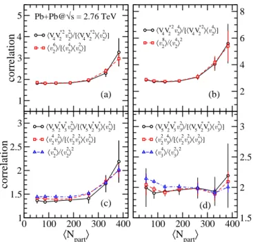
4 1 2 3 4 5
correlation
〈V4V2*2v 2 2 〉/[〈V4V2*2〉〈v 2 2 〉] 〈v 2 6 〉/[〈v 2 4 〉〈v 2 2 〉] 0 100 200 300 400 〈Npart〉 1 1.5 2 2.5 3correlation
〈V5V2*V3*v 2 2 〉/[〈V5V2*V3*〉〈v 2 2 〉] 〈v 2 4 v 3 2 〉/[〈v 2 2 v 3 2 〉〈v 2 2 〉] 〈v 2 4 〉/〈v 2 2 〉2 100 200 300 400 〈Npart〉 1.5 2 2.5 3 〈V5V2*V3*v 3 2 〉/[〈V5V2*V3*〉〈v 3 2 〉] 〈v 2 2 v 3 4 〉/[〈v 2 2 v 3 2 〉〈v 3 2 〉] 〈v 3 4 〉/〈v 3 2 〉2 2 4 6 8 〈V4V2*2v 2 4 〉/[〈V4V2*2〉〈v 2 4 〉] 〈v 2 8〉 /〈v 2 4〉2 Pb+Pb@√s = 2.76 TeV (a) (b) (c) (d)FIG. 3. (Color online) Correlations between event-plane cor-relations and anisotropic flow calculated in AMPT, and tests of Eqs. (9), (10) and (12). Circles connected by solid lines correspond to the left-hand sides, and squares connected by dashed lines correspond to the right-hand sides of these equa-tions.
addition that V4l and V2 are uncorrelated. Equation (8)
then implies the following relation between moments: V4(V2∗)2v22 hV4(V2∗)2i hv22i = v 6 2 hv4 2i hv22i . (9)
This equation relates a mixed correlation between V4and
V2to the fluctuations of elliptic flow: the right-hand side
is the scaled moment m(3)2 introduced in Eq. (6). The
AMPT simulations support Eq. (9) for all centralities, as can be seen in Fig. 3(a). A straightforward generalization of Eq. (9) is obtained using g = v4
2 instead of v22: V4(V2∗)2v42 hV4(V2∗)2i hv42i = v 8 2 hv4 2i 2. (10)
This correlation gives a higher weight to events with large elliptic flow. Equation (10) is also supported by AMPT simulations, as shown in Fig. 3(b).
This discussion can be readily extended to the correla-tion between the 5th harmonic plane and the 2nd and 3rd harmonic planes. We now set f = V5V2∗V
∗ 3 and g = v22 or g = v2 3 and write V5= V5l+ β ′ V2V3, (11)
where V5lis independent of V2and V3and β′ is constant.
One thus obtains V5V2∗V ∗ 3v22 hV5V2∗V ∗ 3i hv22i = v 4 2v32 hv2 2v32i hv22i , V5V2∗V ∗ 3v23 hV5V2∗V ∗ 3i hv23i = v 2 2v43 hv2 2v23i hv32i . (12)
The numerators in the right-hand side are obtained using Eq. (5) with k2 = l2 = 2, k3 = l3 = 1 (first line) and
k2 = l2 = 1, k3 = l3 = 2 (second line). Figs. 3(c)-(d)
again show that these equalities are very well verified by AMPT simulations. One can also use the fact that v2
and v3 are weakly correlated, as seen in Fig. 2, which
leads to the following simplified relations: v4 2v32 hv2 2v32i hv22i ≃ v 4 2 hv2 2i 2, v2 2v34 hv2 2v32i hv23i ≃ v 4 3 hv2 3i 2. (13)
These relations are also satisfied to a good approximation (see Figs. 3(c)-(d)), thus showing that the correlators in Eq. (12) are mostly driven by the fluctuations of v2 and
v3.
V. CONCLUSION
Moments of the distribution of Vn provide a
com-plete set of multiparticle correlation observables, which can be used to probe the physics of flow fluctuations in unprecedented detail. All these moments can be mea-sured using just two subevents separated by a rapidity gap. Moments yield the full information on the multi-particle correlations without resorting to unfolding pro-cedures [14, 46] or event-shape engineering [13, 47, 48]. They can be measured easily at LHC and even with de-tectors having smaller acceptance, and can be directly compared with theoretical calculations. In particular, scaled moments [23] as studied in this paper are typi-cally independent of the details of the acceptance, and reflect global fluctuations. They can be used to further probe the physics of initial-state fluctuations and the hy-drodynamic response of the quark-gluon plasma.
We have shown that the assumption that the correla-tion between V4and V2, and that between V5, V2and V3,
are driven by nonlinear response, yields nontrivial rela-tions between moments, Eqs. (9), (10) and (12). Simu-lations within the AMPT model have shown that these relations are very well satisfied. It is important to test if experimental data confirm these predictions.
ACKNOWLEDGMENTS
This work is funded by CEFIPRA under project 4404-2. JYO thanks the MIT LNS for hospitality and acknowl-edges support by the European Research Council under the Advanced Investigator Grant ERC-AD-267258.
[1] U. Heinz and R. Snellings, Ann. Rev. Nucl. Part. Sci. 63, 123 (2013) [arXiv:1301.2826 [nucl-th]].
[2] M. Luzum, J. Phys. G 38, 124026 (2011) [arXiv:1107.0592 [nucl-th]].
[3] M. Miller and R. Snellings, nucl-ex/0312008.
[4] B. Alver et al. [PHOBOS Collaboration], Phys. Rev. Lett. 98, 242302 (2007) [nucl-ex/0610037].
[5] B. Alver and G. Roland, Phys. Rev. C 81, 054905 (2010) [Erratum-ibid. C 82, 039903 (2010)] [arXiv:1003.0194 [nucl-th]].
[6] G. Aad et al. [ATLAS Collaboration], Phys. Rev. C 90, no. 2, 024905 (2014) [arXiv:1403.0489 [hep-ex]].
[7] M. Luzum and H. Petersen, J. Phys. G 41, 063102 (2014) [arXiv:1312.5503 [nucl-th]].
[8] M. Luzum and J. Y. Ollitrault, Nucl. Phys. A 904-905, 377c (2013) [arXiv:1210.6010 [nucl-th]].
[9] T. Renk and H. Niemi, Phys. Rev. C 89, no. 6, 064907 (2014) [arXiv:1401.2069 [nucl-th]].
[10] L. Yan, J. Y. Ollitrault and A. M. Poskanzer, arXiv:1408.0921 [nucl-th].
[11] D. Teaney and L. Yan, Phys. Rev. C 86, 044908 (2012) [arXiv:1206.1905 [nucl-th]].
[12] L. V. Bravina, B. H. Brusheim Johansson, G. K. Eyyubova, V. L. Korotkikh, I. P. Lokhtin, L. V. Malinina, S. V. Petrushanko and A. M. Sni-girev et al., Phys. Rev. C 89, no. 2, 024909 (2014) [arXiv:1311.0747 [hep-ph]].
[13] J. Jia, J. Phys. G 41, no. 12, 124003 (2014) [arXiv:1407.6057 [nucl-ex]].
[14] G. Aad et al. [ATLAS Collaboration], JHEP 1311, 183 (2013) [arXiv:1305.2942 [hep-ex]].
[15] A. Bilandzic, C. H. Christensen, K. Gulbrandsen, A. Hansen and Y. Zhou, Phys. Rev. C 89, 064904 (2014) [arXiv:1312.3572 [nucl-ex]].
[16] A. Bilandzic, arXiv:1409.5636 [nucl-ex].
[17] Z. W. Lin, C. M. Ko, B. A. Li, B. Zhang and S. Pal, Phys. Rev. C 72, 064901 (2005) [nucl-th/0411110]. [18] R. S. Bhalerao, J. Y. Ollitrault and S. Pal, Phys. Rev. C
88, 024909 (2013) [arXiv:1307.0980 [nucl-th]].
[19] D. Teaney and L. Yan, Phys. Rev. C 90, no. 2, 024902 (2014) [arXiv:1312.3689 [nucl-th]].
[20] N. Borghini and J. Y. Ollitrault, Phys. Lett. B 642, 227 (2006) [nucl-th/0506045].
[21] F. G. Gardim, F. Grassi, M. Luzum and J. Y. Ollitrault, Phys. Rev. C 85, 024908 (2012) [arXiv:1111.6538 [nucl-th]].
[22] K. Aamodt et al. [ALICE Collaboration], Phys. Rev. Lett. 105, 252302 (2010) [arXiv:1011.3914 [nucl-ex]]. [23] R. S. Bhalerao, M. Luzum and J. Y. Ollitrault, Phys.
Rev. C 84, 034910 (2011) [arXiv:1104.4740 [nucl-th]].
[24] A. M. Poskanzer and S. A. Voloshin, Phys. Rev. C 58, 1671 (1998) [nucl-ex/9805001].
[25] M. Luzum and J. Y. Ollitrault, Phys. Rev. C 87, no. 4, 044907 (2013) [arXiv:1209.2323 [nucl-ex]].
[26] R. S. Bhalerao, J. Y. Ollitrault, S. Pal and D. Teaney, arXiv:1410.7739 [nucl-th].
[27] C. Adler et al. [STAR Collaboration], Phys. Rev. C 66, 034904 (2002) [nucl-ex/0206001].
[28] P. Danielewicz and G. Odyniec, Phys. Lett. B 157, 146 (1985).
[29] S. S. Adler et al. [PHENIX Collaboration], Phys. Rev. Lett. 91, 182301 (2003) [nucl-ex/0305013].
[30] L. X. Han, G. L. Ma, Y. G. Ma, X. Z. Cai, J. H. Chen, S. Zhang and C. Zhong, Phys. Rev. C 84, 064907 (2011) [arXiv:1105.5415 [nucl-th]].
[31] J. Xu and C. M. Ko, Phys. Rev. C 84, 044907 (2011) [arXiv:1108.0717 [nucl-th]].
[32] S. Pal and M. Bleicher, J. Phys. Conf. Ser. 420, 012027 (2013) [arXiv:1209.0335 [nucl-th]].
[33] S. Pal and M. Bleicher, Phys. Lett. B 709, 82 (2012) [arXiv:1201.2546 [nucl-th]].
[34] W. T. Deng, X. N. Wang and R. Xu, Phys. Rev. C 83, 014915 (2011) [arXiv:1008.1841 [hep-ph]].
[35] M. Luzum, Phys. Lett. B 696, 499 (2011) [arXiv:1011.5773 [nucl-th]].
[36] G. Aad et al. [ATLAS Collaboration], Eur. Phys. J. C 74, no. 11, 3157 (2014) [arXiv:1408.4342 [hep-ex]]. [37] N. Borghini, P. M. Dinh and J. Y. Ollitrault, Phys. Rev.
C 64, 054901 (2001) [nucl-th/0105040].
[38] J. Adams et al. [STAR Collaboration], Phys. Rev. C 72, 014904 (2005) [nucl-ex/0409033].
[39] A. Bilandzic, R. Snellings and S. Voloshin, Phys. Rev. C 83, 044913 (2011) [arXiv:1010.0233 [nucl-ex]].
[40] A. Bzdak, P. Bozek and L. McLerran, Nucl. Phys. A 927, 15 (2014) [arXiv:1311.7325 [hep-ph]].
[41] S. A. Voloshin, A. M. Poskanzer, A. Tang and G. Wang, Phys. Lett. B 659, 537 (2008) [arXiv:0708.0800 [nucl-th]]. [42] K. Aamodt et al. [ALICE Collaboration], Phys. Rev.
Lett. 107, 032301 (2011) [arXiv:1105.3865 [nucl-ex]]. [43] J. Y. Ollitrault, Phys. Rev. D 46, 229 (1992).
[44] J. Jia and D. Teaney, Eur. Phys. J. C 73, 2558 (2013) [arXiv:1205.3585 [nucl-ex]].
[45] P. Huo, J. Jia and S. Mohapatra, Phys. Rev. C 90, no. 2, 024910 (2014) [arXiv:1311.7091 [nucl-ex]].
[46] B. Alver et al. [PHOBOS Collaboration], Phys. Rev. Lett. 104, 142301 (2010) [nucl-ex/0702036].
[47] J. Schukraft, A. Timmins and S. A. Voloshin, Phys. Lett. B 719, 394 (2013) [arXiv:1208.4563 [nucl-ex]].
[48] A. Dobrin [ALICE Collaboration], Nucl. Phys. A 904-905, 455c (2013) [arXiv:1211.5348 [nucl-ex]].