Structured prediction and generative modeling using neural networks

(1)

Universit´e de Montr´eal

Structured Prediction and Generative Modeling using Neural Networks

par Kyle Kastner

Département d’informatique et de recherche opérationnelle Faculté des arts et des sciences

Mémoire présenté à la Faculté des arts et des sciences en vue de l’obtention du grade de Maˆıtre ès sciences (M.Sc.)

en informatique

Aoˆut, 2016

c

(2)

Résumé

Cette thèse traite de l’usage des Réseaux de Neurones pour modélisation de données séquentielles. La fa¸con dont l’information a été ordonnée et structurée est cruciale pour la plupart des données. Les mots qui composent ce paragraphe en constituent un exemple. D’autres données de ce type incluent les données audio, visuelles et génomiques. La Prédiction Structurée est l’un des domaines traitant de la modélisation de ces données. Nous allons aussi présenter la Modélisation Générative, qui consiste à générer des points similaires aux données sur lesquelles le modèle a été entraˆıné.

Dans le chapitre 1, nous utiliserons des données clients afin d’expliquer les concepts et les outils de l’Apprentissage Automatique, incluant les algorithmes standards d’apprentissage ainsi que les choix de fonction de coût et de procédure d’optimisation. Nous donnerons ensuite les composantes fondamentales d’un R´ e-seau de Neurones. Enfin, nous introduirons des concepts plus complexes tels que le partage de paramètres, les Réseaux Convolutionnels et les Réseaux Récurrents. Le reste du document, nous décrirons de plusieurs types de Réseaux de Neurones qui seront à la fois utiles pour la prédiction et la génération et leur application à des jeux de données audio, d’écriture manuelle et d’images

Le chapitre 2.2 présentera le Réseau Neuronal Récurrent Variationnel (VRNN pour variational recurrent neural network). Le VRNN a ´eté développé dans le but de générer des échantillons semblables aux exemples de la base d’apprentissage. Nous présenterons des modèles entraˆınées de manière non-supervisée afin de générer du texte manuscrites, des effets sonores et de la parole. Non seulement ces modèles prouvent leur capacité à apprendre les caractéristiques de chaque type de données mais établissent aussi un standard en terme de performance.

Dans le chapitre3sera présenté ReNet, un modèle récemment développé. ReNet utilise les sorties structurées d’un Réseau Neuronal Récurrent pour classifier des objets. Ce modèle atteint des performances compétitives sur plusieurs tâches de reconnaissance d’images, tout en utilisant une architecture con¸cue dès le départ pour de la Prédiction Structurée. Dans ce cas-ci, les résultats du modèle sont utilisés simplement pour de la classification mais des travaux suivants (non-inclus ici) ont utilisé ce modèle pour de la Prédiction Structurée.

Enfin, au Chapitre 4 nous présentons les résultats récents non-publiés en gén´ e-ration acoustique. Dans un premier temps, nous fournissons les concepts musicaux et représentations numériques fondamentaux à la compréhension de notre approche et introduisons ensuite une base de référence et de nouveaux résultats de recherche

(3)

avec notre modèle, RNN-MADE. Ensuite, nous introduirons le concept de synthèse vocale brute et discuterons de notre recherche en génération. Dans notre dernier Chapitre, nous présenterons enfin un résumé des résultats et proposerons de nou-velles pistes de recherche.

Mots clés : r´eseaux de neurones, apprentissage automatique, apprentissage de représentations profondes, apprentissage supervisé, modèles génératifs, prédiction structurée

(4)

Summary

In this thesis we utilize neural networks to effectively model data with sequen-tial structure. There are many forms of data for which both the order and the structure of the information is ncredibly important. The words in this paragraph are one example of this type of data. Other examples include audio, images, and genomes. The work to effectively model this type of ordered data falls within the field of structured prediction. We also present generative models, which attempt to generate data that appears similar to the data which the model was trained on. In Chapter 1, we provide an introduction to data and machine learning. First, we motivate the need for machine learning by describing an expert system built on a customer database. This leads to a discussion of common algorithms, losses, and optimization choices in machine learning. We then progress to describe the basic building blocks of neural networks. Finally, we add complexity to the mod-els, discussing parameter sharing and convolutional and recurrent layers. In the remainder of the document, we discuss several types of neural networks which find common use in both prediction and generative modeling and present examples of their use with audio, handwriting, and images datasets. In Chapter 2.2, we intro-duce a variational recurrent neural network (VRNN). Our VRNN is developed with to generate new sequential samples that resemble the dataset that is was trained on. We present models that learned in an unsupervised manner how to generate handwriting, sound effects, and human speech setting benchmarks in performance. Chapter 3 shows a recently developed model called ReNet. In ReNet, inter-mediate structured outputs from recurrent neural networks are used for object classification. This model shows competitive performance on a number of image recognition tasks, while using an architecture designed to handle structured pre-diction. In this case, the final model output is only used for simple classification, but follow-up work has expanded to full structured prediction.

Lastly, in Chapter 4 we present recent unpublished experiments in sequential audio generation. First we provide background in musical concepts and digital representation which are fundamental to understanding our approach and then introduce a baseline and new research results using our model, RNN-MADE. Next we introduce the concept of raw speech synthesis and discuss our investigation into generation. In our final chapter, we present a brief summary of results and postulate future research directions.

Keywords: neural networks, machine learning, deep learning, supervised learn-ing, generative modellearn-ing, structured prediction

(5)

List of Figures

1.1 Example decision process for deciding “good” or “bad” customers . . 4

1.2 Function y = x2 . . . 16

1.3 Moving down the gradient to a minimum . . . 16

1.4 Descending from the other side . . . 17

1.5 Descending non-convex function, by “skipping” the problem region . 17 1.6 Sigmoid function sigm(x) = 1 1+exp−x . . . 20

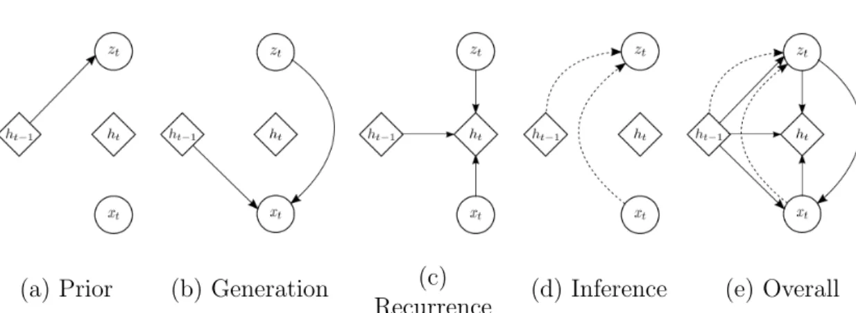
1.7 Graphs demonstrating nonlinear functions from left to right: Sig-moid (_1+exp1 _−x), tanh (1_1+exp−exp−2x_−2x), and rectified linear (0 if x < 0 else x) 21 2.1 Graphical illustrations of each operation of the VRNN: (a) comput-ing the conditional prior uscomput-ing Eq. (2.5); (b) generatcomput-ing function using Eq. (2.6); (c) updating the RNN hidden state using Eq. (2.7); (d) inference of the approximate posterior using Eq. (2.9); (e) overall computational paths of the VRNN. . . 35

2.2 The top row represents the diﬀerence δtbetween µz,tand µz,t−1. The middle row shows the dominant KL divergence values in temporal order. The bottom row shows the input waveforms. . . 39

2.3 Examples from the training set and generated samples from RNN-GMM and VRNN-Gauss. Top three rows show the global waveforms while the bottom three rows show more zoomed-in waveforms. Sam-ples from (b) RNN-GMM contain high-frequency noise, and samSam-ples from (c) VRNN-Gauss have less noise. We exclude RNN-Gauss, because the samples are almost close to pure noise. . . 40

2.4 Handwriting samples: (a) training examples and unconditionally generated handwriting from (b) RNN-Gauss, (c) RNN-GMM and (d) VRNN-GMM. The VRNN-GMM retains the writing style from beginning to end while RNN-Gauss and RNN-GMM tend to change the writing style during the generation process. This is possibly be-cause the sequential latent random variables can guide the model to generate each sample with a consistent writing style. . . 41

3.1 A one-layer ReNet . . . 47

3.2 The ReNet network used for SVHN classification. . . 50

(9)

4.2 Example Markov chain generation (temperature 1000, Markov order

6) in ABC format . . . 65

4.3 Model diagram for one step in RNN-MADE . . . 66

4.4 Piano roll plot, training data . . . 68

4.5 Piano roll plot, generated data . . . 68

4.6 Example waveform . . . 71

4.7 Spectrogram of example utterance from the training set . . . 75

(10)

List of Tables

1.1 Example customer data. . . 2

1.2 Extended customer data . . . 3

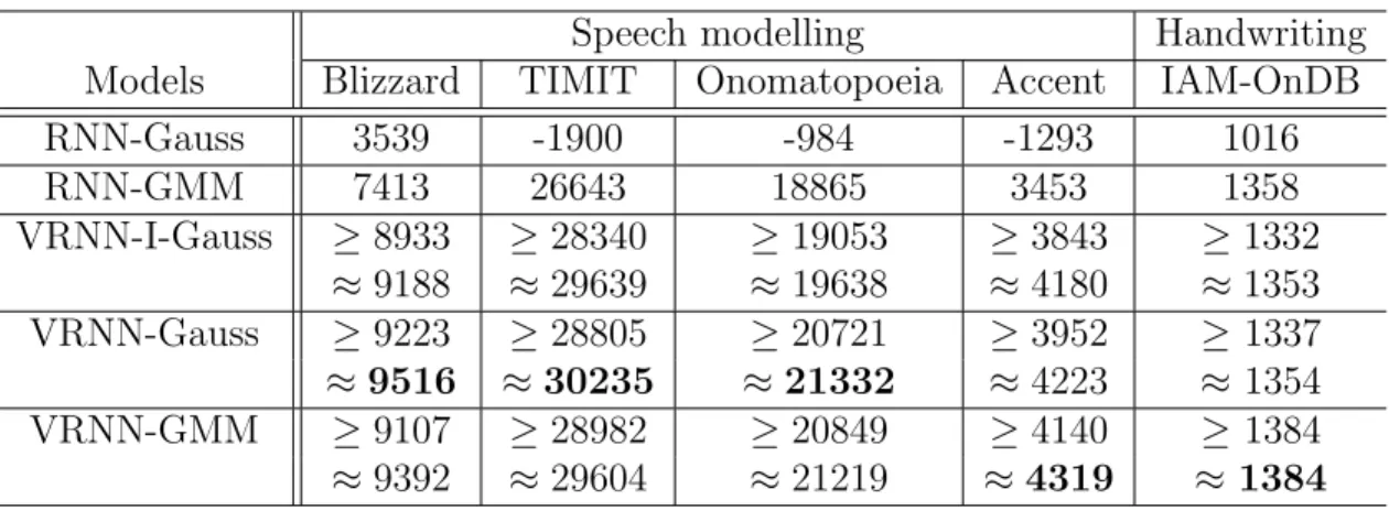
2.1 Average log-likelihood on the test (or validation) set of each task. . 37

3.1 Model architectures used in the experiments. Each row shows re-spectively the number of ReNet layers, the size of the patches, the number of neurons of each ReNet layer, the number of fully con-nected layers, the number of neurons of the fully concon-nected layers, their activation function and the data augmentation procedure em-ployed. . . 52

3.2 Generalization errors obtained by the proposed ReNet along with those reported by previous works on each of the three datasets. ⋆ denotes a convolutional neural network. We only list the results reported by a single model, i.e., no ensembling of multiple models. In the case of SVHN, we report results from models trained on the Format 2 (cropped digit) dataset only. . . 53

(11)

List of Abbreviations

AE Auto-Encoder

CNN Convolutional Neural Network GD Gradient Descent

GRU Gated Recurrent Unit GMM Gaussian Mixture Model HMM Hidden Markov Model KLD Kullback-Liebler Divergence LSTM Long-Short Term Memory

MLE Maximum Likelihood Estimation MLP Multi-Layer Perceptron

MSE Mean Squired Error

NADE Neural Autoregressive Density Estimator NLL Negative Log-Likelihood

PMF Probability Mass Function PDF Probability Density Function RNN Recurrent Neural Network SGD Stochastic Gradient Descent VAE Variational Auto-Encoder XE Cross Entropy

(12)

Acknowledgments

I am extremely grateful for an amazing set of family, friends, colleagues, and advisers without whom my work would not be possible.

Johanna Hansen, thank you for your continued love, support, and partnership. I would not be able to do any of this without you. I am blessed with an incredible immediate and extended family whose continued love, support, and strength has helped me every step of the way. Thanks to my mother, Sandra; father, Victor; and sister, Courtney.

Thank you to Dr. Roland Memisevic, Dr. Aaron Courville, and Dr. Yoshua Ben-gio for serving as outstanding advisers. Your direction, research mentorship, and guidance has allowed me to grow as a researcher and follow the path I am on today. To my many friends, co-authors, co-workers, and colleagues (alphabetically): Adam Roberts, Adriana Romero, Alex Lamb, Alexandre Abraham, Amjad Alma-hairi, Anna Huang, Arnaud Bergeron, Barron Bichon, Bart van Merriënboer, Ben Poole, Brandon Sammons, ¸Caglar Gül¸cehre, Casper Kaae Sønderby, César Lau-rent, Chris Smith, Christof Angermueller, Cinjon Resnick, Colin Raffel, Colin Vaz, Curtis ”Fjord” Hawthorne, Daniel Trejo, Daniel Jiwoong Im, David Ha, David Krueger, David Warde-Farley, Dmitriy Serdyuk, Dzmitry Bahdanau, Elvis Dohma-tob, Eduardo Gonzalez, Eugene Belilovsky, Fabian Pedregosa, Faruk Ahmed, Felix Hill, Francesco Visin, Fred Bertsch, Frédéric Bastien, Guillaume Alain, Harm de Vries, Ishaan Gulrajani, Ishmael Belghazi, Iulian Vlad Serban, Jacob Limmer, Jan Chorowski, Jesse Engel, João Felipe Santos, Jörg Bornschein, José Sotelo, Juny-oung Chung, Kelvin Xu, Kratarth Goel, Kyunghyun Cho, Laurent Dinh, Li Yao, Luke Vilnis, Marcelo Grave, Mark Pillion, Mary Otto, Mathieu Germain, Matthew Coursen, Mehdi Mirza, Michael Eickenberg, Michael Talbert, Mohammad Pezesh-ski, Myriam Côté, Natasha Jaques, Nicolas Ballas, Negar Rostamzadeh, Orhan Firat, Pascal Lamblin, Patrick Sammons, Pierre-Luc Carrier, Philemon Brakel, Rick Parker, Sam Stavinoha, Sebastian Öberg, Shawn Tan, Simon Receveur, Sina Honari, Søren Sønderby, Soroush Mehri, Stanislas Lauly, Sungjin Ahn, Tim Cooi-jmans, Vincent Dumoulin, and Yann Dauphin; Thank you for everything you do. Thank you to Mohammad Pezeshski for showing me how to use this thesis template by example and to Nicolas Chapados for providing the thesis template. Thank you

(13)

to Laurent Dinh for translating the summary portion of this thesis. Thank you also to C´eline Begin for all her patience during the thesis submission process and for her organizational help during my studies.

In addition, thanks to the rest of my friends and coworkers in MILA, my pre-vious workplaces, the scikit-learn team, and the internet at large. I am sure I missed some people I shouldn’t have forgotten. Thanks to all of you.

To all my wonderful teachers Matt Popnoe, Rex Ewert, Richard Roper, Butch Crudginton, Dr. Donald Olson, Dr. Heather Galloway, Dr. Michael Casey, Dr. Stan McClellan, Dr. William Stapleton, Dr. Jim Lansford, and Dr. Sos Agaian. Thank you for so much education and inspiration.

To my friends and mentors from SwRI (some now elsewhere), I wouldn’t be here without you. AF, SB, DC, DH, BM, AH, GM, BR, JJ, MG, RC, KB, DVR, DF, RH, KD, JS, TS, BB, AE, CZ, HO, BN, JP, JN along with many others.

I also want to express an extra thanks to my internship mentors: Ga¨el Varoquaux and Olivier Grisel at INRIA Parietal, Bhuvana Ramabhadran and Ewout van den Berg at IBM Research, and Douglas Eck and Mike Schuster at Google Brain. To my friends, family, and mentors who are no longer with us, RIP and thank you for everything.

Finally, the work reported in this thesis would not have been possible without the financial support from: Ubisoft, Samsung, IBM, NSERC, Calcul Quebec, Compute Canada, the Canada Research Chairs and CIFAR.

(14)

1

Introduction

1.1 Overview

Machine learning is an important part of modern computer science, with appli-cations across many industries including commerce, finance, logistics, agriculture, and education. There are many detailed references for deeply understanding ma-chine learning such as Bishop (2006), Hastie et al. (2001), Murphy (2012), and

Goodfellow et al. (2016). In this introductory chapter, we simply strive to give an overview of the core concepts and terminology necessary for understanding the basics of the later chapters. In this work we will cover some recent advances in the subfields of machine learning known as structured prediction and generative mod-eling. Structured prediction refers to using machine learning to predict structured elements such as vectors or sets, rather than single values. Generative modeling means that we desire to use our techniques to generate new outputs similar to the inputs. The combination of structured prediction can be used to generate things like audio, handwriting, images, and text. We approach these problems using deep learning techniques with neural networks. Structured prediction and generative modeling will be covered in more detail later, but first we will provide background on machine learning in general. Machine learning can be partly defined by exploring one of its component terms: learning.

What is learning?

One place to begin in our quest to understand learning is the dictionary defi-nition. The Myriam-Webster dictionary defines learning as: the activity or process of gaining knowledge or skill by studying, practicing, being taught, or experiencing something (myr,2016). The most important aspect of this definition is that study-ing, teachstudy-ing, practicstudy-ing, or experiencing all involve taking these actions over some information. For our purposes the information that we study is known as data. We

(15)

expect that the ability to make good decisions will improve with algorithmic study (through a learning algorithm) of a particular type data. In machine learning we attempt to make good decisions about data, by using learning algorithms to study the data in question.

What is data?

Data is a catch-all term used to describe any kind of information about an object, process, or concept. In the context of machine learning data is the de-scription of what we want to learn about, for example: the purchase history of a customer, the pixels of an image, the text of a sentence, some recordings from election speeches, or any other domain-dependent information that could be useful

Shannon (1948). A typical way of representing data in machine learning is as a collection of attributes, or features. These features describe some characteristics of the thing being measured. Let’s envision a dataset from a department store as an example. The store manager wishes to learn more about his customers by investigating his historical records about their shopping habits. In the context of machine learning, each customer is a sample and the customer’s shopping records are known as features. Features may include details about the customer such as the last item purchased, the total of their last bill, and the number of years they have been a customer. In this simple set of data, we can represent each customer with three numerical features: item id, prev bill, n years.

Table 1.1 – Example customer data

item id prev bill n years Customer A 11764 1000.00 0.6 Customer B 9718 243.16 5.12

Customer C 42 156.19 3.3

Table 1.1 shows a common format for data in a dataset. In this representation, the vertical dimension of the array is the sample axis, while the horizontal axis is the feature axis. In general, the feature vectors for each sample can be stacked to make a data matrix (often denoted simply as x), and later fed to any number of learning algorithms. There are many other ways to represent data which can

(16)

capture additional structure in data such as images, text, graphs, audio, or video that certain algorithms can use for better learning. Before discussing learning algorithms in detail, we must first describe what we wish to learn in the first place: decisions.

What are decisions?

In the preceding paragraphs, we introduced decisions as the basis which the act of studying, teaching, practicing, or experiencing was meant to improve. However, it is not necessary to have learning algorithms in order to make a decision. Let us construct an example using the department store data which was introduced in Table 1.1.

Table 1.2 – Extended customer data

item id prev bill n years good bad

Customer A 11764 1000.00 0.6 1

Customer B 9718 243.16 5.12 0

Customer C 42 156.19 3.3 ?

Suppose in addition to the information in Table 1.1, we were also given addi-tional information about each customer, namely whether each customer was “good” (0) or “bad” (1) for the business. We could add this information to the dataset, resulting in a new table, Table 1.2.

Notice in particular that Customer C has unknown information in the “good bad” column, but it is believable that we might want to predict or infer that attribute for Customer C. One way to do this might be to find the employee who created the “good bad” attributes for the other customers, and ask them to encode their logic

for making their decision on “good” or “bad” into a procedure, or function.

This function (shortened to f ()) should take the data we have now (x) for each customer, and try to output the value for “good bad” (sometimes called the labels or targets typically denoted y), such that for existing customers with known values for “good bad”, yc = f (xc) where c is shorthand to reference the features

(xc) and labels (yc) for each customer. For Customer C, we have no true value for

(17)

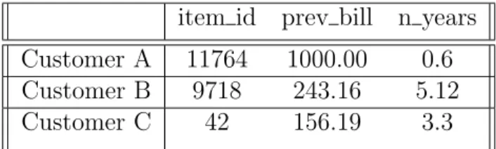
n_years > 2 “good” prev_bill > 300 prev_bill > 500 “bad” “good” “bad” True True True False False False

Figure 1.1 – Example decision process for deciding “good” or “bad” customers

is correct on Customers A and B. However if the function is working well, it is now possible to predict the “good bad” attribute for Customer C or any other customer with the same feature information. If customers are added to the dataset later, and have all their features input this function could then predict the “good bad” attribute and add it to the database. The logic for such a decision might be simple, as in Figure 1.1.

Motivations for machine learning

The logic for predicting “good” or “bad” customers is an example of something known as an expert system (Russel and Norvig, 2003). Variants of these expert systems, using a number of diﬀerent algorithms, have been employed to make machine decisions since the dawn of computing. The solution shown in Figure 1.1

shows an algorithm called a decision tree with explicitly set rules. Decision trees in particular show up in a variety of contexts, and those employing and coding handcrafted decision trees are often unaware that they have already implemented a direct precursor to machine learning by using machine decisions indirectly based on data (after being filtered through the mind of one or many employees). The details of decision trees will not be covered in detail here, but Hastie et al. (2001)

(18)

is an excellent reference for this algorithm and various extensions.

The primary diﬀerence between this hypothetical system and a machine learning approach would be having the machine learn the decision thresholds directly, rather than requiring the programmer or another expert to specify the rule manually. Many large codebases in open source and enterprise have files of “magic code”, filled with complex if-else statements and unknown or undocumented constants for making choices at each branch. These are real-world examples of “expert systems”, and in many cases machine learning techniques can greatly improve performance. Machine learning models can often discover new or unknown relationships in the data which are not obvious to the human expert.

From a machine learning perspective, expert systems are not considered a learn-ing system. The programmer(s) have input the entire logic explicitly into the deci-sion process, and it is not clear how these rules were derived without explanations and expertise. Indeed, it is believable that the rules that work for Customers A and B might not work in every circumstance. More customer data and labels, more features, or both may be necessary to make rules which are more general. As in-formation for customers is gathered, the rules which exist may be worse than a potential set of new rules, especially as more features and labels are obtained.

One way to continuously improve this system would be to dedicate one employee fully to creating and testing new rules. As customers and features are added to the data matrix, this employee could potentially write better rules. Eventually the number of customers and features might overwhelm a single employee, and a team would needed to do this job. Soon, a whole section of the company might be entirely focused on writing new rules for this predictive system, an expensive proposition (Brooks, 1995).

What if we could instead write higher level routines, so that the machine itself could learn basic rules from data? This could scale to much larger problems, without incurring a larger overhead beyond increased computer time. This is the basic premise (and promise) of machine learning.

(19)

1.2 Types of Learning

Using the descriptions from the previous section, we have loosely defined learn-ing as the development of a function f () which takes in data, and outputs desired information. This function must have some internal values which can be learned or modified, typically called parameters and denoted by θ (theta). In the previ-ous example, the parameters of θ would be the thresholds for each “if” statement, but usually what parameters do is dependent on the algorithm contained inside f (). This means the function f () is actually a function of both the inputs and the learned parameters θ, so it can also be written fθ() or f (a, θ). Most machine

learn-ing references don’t directly denote θ and instead leave it as a known assumption. There are also approaches which do not have parameters. Approaches without parameters are called (non-parametric) functions. For the moment, we will limit our discussion to parametric approaches. Machine learning attempts to solve many tasks, but generally we can categorize learning into two broad types: supervised learning and unsupervised learning.

Supervised learning is focused on learning a mapping between data and label. The label can be a numeric value, as in our department store example. The data can also be any number of human created or curated values such as pixels or words. We continue the previous notation, and denote general supervised tasks as attempting to learn yi = f (xi) for each sample i with “supervision” values in the

dataset. This function can then be used to label new data samples without a known label. Supervised learning is also called predictive modeling in some references.

Unsupervised learning, in contrast to supervised learning, is explicitly focused on learning more suitable features, sometimes called representations, without spe-cific labels on the data. Unsupervised tasks often attempt to learn forms of com-pression, such as ˆxi = f (xi). Specifically ˆxi is a reconstruction of xi after being

passed through an information bottleneck, so that the function must learn to com-press information. This comcom-pression is important since the alternative is the trivial solution of xi = xi, which should be avoided. Learning to reconstruct a part of

some data, given its surrounding information (sometimes called context) is another way to learn good representations for many types of data. Unsupervised learning is also called generative modeling in many settings, and specific approaches explicitly attempt to learn generative distributions of the data. We will cover more on these

(20)

approaches in later chapters.

Subgroups of Supervised and Unsupervised Learning

In addition to the broad categorizations of unsupervised and supervised learn-ing, there are sub-groupings such as classification, regression, and density esti-mation. Specifically, classification and regression are diﬀerent types of supervised learning, while the basic forms of density estimation are unsupervised tasks. Clas-sification is used to denote tasks which involve categorizing data points into one of K possible buckets, or classes. Regression, in the context of machine learning, is a common task which is popular in the statistics literature. Regression algorithms attempt to predict a real value for each input xi. Density estimation is a

tech-nique for fitting probability densities to data, to determine underlying structure. Clustering algorithms are generally categorized as a subset of density estimation.

Bishop (2006) and Hastie et al. (2001) are both excellent references for listings of diﬀerent techniques in these groups and subgroups of machine learning.

In the example case from the previous section, we wanted a function to predict the “good bad” attribute for each customer, which is one of two values in the set{0, 1}. Because this task requires learning a function to map the data x to a human labeled attribute y, which is one of K possibilities (in this case K = 2), we broadly file this task under the heading of supervised classification.

1.3 A Formal Definition of Learning

One common mathematical framework for machine learning is to define the problem of discovering the optimal parameters (θ∗) as an optimization problem. The fundamental problem then becomes minimizing risk, where risk is the inte-gration of some loss function between the true values y and some function f (x, θ), where the integration is with respect to the joint probability distribution of x and y. This framework was defined in Vapnik(1991), and serves as clear reading material covering much of the basis for machine learning as optimization.

R(θ) = ∫

(21)

Noting that the joint probability p(x, y) can be rewritten using Bayes rule, we see that p(x, y) = p(x|y)p(y) = p(y|x)p(x). This joint probability is unknown for most problems of interest, since we usually do not know the underlying data distributions p(x) or p(y). Our only available source of information is in the training set, yet we must approximate this integral somehow. Replacing the problem of risk minimization with empirical risk minimization, or minimizing the summed loss over the training set (sometimes called the empirical data distribution), is our best approximation to the integral in Equation1.1.

ER(θ) = 1 l l ∑ i=1 L(yi, f (xi, θ)) (1.2)

Thus, the desired set of parameters θ∗is the set of θ that minimize the empirical risk ER(θ). θ∗ = argminy l ∑ i=1 L(yi, f (xi, θ)) (1.3)

These general notions form much of the intuition behind machine learning as optimization, and can be extended in interesting ways to improve results on struc-tured problems (Bahdanau et al.,2015). It is important to note that the parameters θ∗ which are optimal on one data subset may not generalize to new subsets. Indeed much of the “art” in machine learning is understanding and minimizing diﬀerences in performance between the set used for loss minimization (the so called train-ing set) and the application domain. This can partially be done through careful composition of losses, algorithms, regularization, and optimization techniques.

1.4 Losses

After discussing the empirical risk minimization framework, it is necessary to define actual functions to use for L(y, f (x, y)). In many cases we use the function f (x, y) to model conditional probability distributions pθ(y|x). This directly leads

to costs which have a probabilistic interpretation when taking the maximum like-lihood estimator (MLE) over whatever output distribution is assumed for pθ(y|x)

(22)

In many common cases, the cost can be derived as the negative log-likelihood between the data and the current model distribution. Negative log-likelihood is also commonly known as cross-entropy, and the two terms are commonly interchanged in machine learning literature. In the standard problem setting data doesn’t change during learning, so reducing the cross-entropy amounts to improving the likelihood of pθ(y|x) with respect to the data. This is also equivalent to minimization of the

Kullback-Liebler divergence (KLD) between the empirical data distribution and the model distribution, as demonstrated in Nowak(2009). Thus optimizing cross-entropy corresponds to reducing the gap between the empirical distribution and the model. The θ∗ corresponding to the lowest cross-entropy is therefore a best estimate for the parameters p∗_θ(y|x), under the distribution assumptions of the cost. We will re-derive several common costs using this general principle.

1.4.1 Relationship between KLD and MLE

Beginning with two distributions p(x) (the empirical distribution) and q(x) (the model distribution), we first state the KLD (Nowak, 2009).

DKL(p(x)||q(x)) = ∫ p(x) log p(x)dx− ∫ p(x) log q(x)dx (1.4) = ∫ p(x) logp(x) q(x)dx (1.5) =Ex∼p[log p(x) q(x)] (1.6) =Ex∼p[log p(x)− log q(x)] (1.7)

(23)

points. θ∗ = arg max θ l ∏ i=1 q(xi) (1.8) = arg max θ l ∑ i=1 log q(xi) (1.9) = arg min θ 1 l l ∑ i=1 − log q(xi) (1.10) ∼= arg min θ El→∞,x∼p[− log q(x)] (1.11)

The last approximate equality occurs due to the “law of large numbers”, as l goes to ∞. Note that both the KLD and MLE have a term related to the expectation of the negative log probability of the model distribution (q(x)). The KLD between these two probability distributions is always positive, and only 0 if they exactly match. Going back to the original formulation for DKL(p(x)||q(x)) we can also

reformulate the terms in another way.

DKL(p(x)||q(x)) = ∫ p(x) log p(x)dx− ∫ p(x) log q(x)dx (1.12) =−H(p(x)) + XE(p(x), q(x)) (1.13) = C + XE(p(x), q(x)) (1.14)

Here Equation1.12shows that the KLD is a combination of the negative entropy (−H(p(x)) of the empirical data distribution, and the cross-entropy XE(p(x), q(x)) between the empirical data and our model distribution. Because we are optimizing only q(x), we can eﬀectively ignore the entropy term (later named C and combined with other constant terms), as it will not change. This means minimizing the KLD between p(x) and q(x) is equivalent to minimizing the cross-entropy between p(x) and q(x). p(x) is never changing, so minimizing− log q(x) (also called the negative log-likelihood) also minimizes cross-entropy.

In each case, some shorthand will be denoted for the last line of the loss so the final formulation closer resembles the implementation in code. In the classification case (cross-entropies) this involves yt the true labels, and yp the predicted labels.

(24)

1.4.2 Bernoulli Cross-entropy

Bernoulli cross-entropy is named as such because the labels are assumed to be from a Bernoulli distribution (Buja et al., 2005), which is often used in two-class classification problems. The Bernoulli distribution represents a random variable which has two possible values: k = {0, 1}, with occurrence probability pk and

1− pk, respectively. p =    pk, if k = 1 1− pk, if k = 0 (1.15) DKL(p(x)||q(x)) = ∫ p(x) log p(x)− ∫ p(x) log q(x) (1.16) =∑p(x) log p(x)−∑p(x) log q(x) (1.17) = C− ∑ c∈0,1 p(x) log q(x) (1.18) =−∑ c∈0,1 p(x) log q(x) + C (1.19) ∼= −∑ c∈0,1 p(x) log q(x) (1.20) ∼= −p(x) log q(x) − (1 − p(x)) log(1 − q(x)) (1.21) ∼= l ∑ i=0

−yt[i]log yp(xi)− (1 − yt[i]) log(1− yp(xi)) (1.22)

The integrals of the KLD become sums because of the discrete nature of the distribution. The final derivation comes due to the definition of the Bernoulli probability mass function (PMF) Equation1.15. Minimizing the final loss term (C can be ignored because it is constant with respect to q(x)) will match the model predictions yp = f (x). The function f (x) is a floating point prediction between

0 and 1. This will, after optimizing parameters θ, attempt to match the labeled dataset yt, which has values of either 0 or 1.

(25)

1.4.3 Categorical Cross-entropy

The categorical (also known as multinoulli) distribution is a K class general-ization of the two class Bernoulli (Hastie et al., 2001). Generally the prediction is a vector of probabilities for each class, so the target yt is a class in the one-hot

representation as a vector of length K, k = {0 · · · K}, where K is the number of classes. For example (with 5 classes) 0 becomes [1, 0, 0, 0, 0], 1 becomes [0, 1, 0, 0, 0], and so on. v[c] will generally refer to indexing into this vector v, assuming indices start from 0. In this manner, we refer to pk as a set of K values which form a valid

discrete probability distribution, so pk[c] refers to the cth index into pk.

p =    pk[c], if c = k 0, if c̸= k (1.23) DKL(p(x)||q(x)) = ∑ p(x) log p(x)−∑p(x) log q(x) (1.24) = C − ∑ c∈0...K p(x) log q(x) (1.25) =− ∑ c∈0...K p(x) log q(x) + C (1.26) ∼= − ∑ c∈0...K p(x) log q(x) (1.27) ∼= − ∑ c∈0...K p(x)[c] log q(x)[c] (1.28) ∼= − l ∑ i=0 ∑ c∈0...K yt[i][c] log yp(xi)[c] (1.29)

1.4.4 Gaussian Negative Log-Likelihood

Another approach is to make a Gaussian assumption, using the probability distribution shown in Equation 1.30.

p = 1

(2πσ)12

exp(−(x− µ)

2

2σ2 ) (1.30)

We track the parameters of p(x) as µ1 and σ1, and the parameters of q(x) as

(26)

DKL(p(x)||q(x)) = ∫ p(x) log p(x)dx− ∫ p(x) log q(x)dx (1.31) = ∫ p(x) logp(x) q(x)dx (1.32) = ∫ p(x) log 1 (2πσ2 1) 1 2 exp(− (x−µ1)2 2σ2 1 ) 1 (2πσ2 2) 1 2 exp(− (x−µ2)2 2σ2 2 ) dx (1.33) = ∫ p(x) log 1 (2πσ2 1) 1 2 exp(−(x− µ1) 2 2σ2 1 )dx (1.34) − ∫ p(x) log 1 (2πσ2 2) 1 2 exp(−(x− µ2) 2 2σ2 2 )dx (1.35) =−Hg(x)− ∫ p(x) log 1 (2πσ2 2) 1 2 exp(−(x− µ2) 2 2σ2 2 ) (1.36) =−Hg(x) + 1 2log(2πσ 2 2)− ∫ p(x) log exp(−(x− µ2) 2 2σ2 2 )dx (1.37) =−Hg(x) + 1 2log(2πσ 2 2) + ∫ p(x)(x− µ2) 2 2σ2 2 dx (1.38) =−Hg(x) + 1 2log(2πσ 2 2) + 1 2σ2 2 ( ∫ p(x)x2dx− ∫ p(x)2xµ2dx + ∫ p(x)µ2₂dx) (1.39) =−Hg(x) + 1 2log(2πσ 2 2) + 1 2σ₂2(E[x 2_]_{− 2E[x]µ} 2 + µ22) (1.40) =−Hg(x) + 1 2log(2πσ 2 2) + 1 2σ2 2 (E[x]− µ2)2 (1.41) =−Hg(x) + 1 2log(2π) + 1 2log(σ 2 2) + 1 2σ2 2 1 l l ∑ i=0 (xi− µ2)2 (1.42) = C + log(σ2) + 1 2σ2 2 1 l l ∑ i=0 (xi− µ2)2 (1.43) = log(σ2) + 1 2σ2 2 1 l l ∑ i=0 (xi− µ2)2 (1.44) = l ∑ i=0 log(σ2(xi)) + 1 2(σ2(xi))2 (xi− µ2(xi))2 (1.45)

(27)

Here we see that a model with Gaussian negative log-likelihood would need to output two things, µ2(xi) and σ2(xi) (Nowak, 2009; Bishop, 2006). In practice

it is often necessary to restrict the minimum variance allowed. This is because optimizing this cost can improve arbitrarily by shrinking σ2(xi) toward 0 if µ2(xi)

lies directly on the data point.

1.4.5 Mean Squared Error

Given the previous derivation, it is easy to see that if σ2 is assumed constant,

the final result is the well known equation for mean squared error where µ2(xi)

is the prediction of the model (Hastie et al., 2001). We typically set σ2 = 1 for

simplicity, but any constant value can be used and then factored out.

min DKL(p(x)||q(x)) = min θ 1 l l ∑ i=0 (xi − µ2(xi))2 (1.46)

1.5 A Basic Model

The method that we use to calculate the predictions f () (or q(x) in the previous notation) is often called a model. One of the simplest models is the linear model which is a simple linear transformation of the input (Strang, 2006). Defining the number of features, m, in each sample, xi, with a total of n samples, results in x

(the dataset) having shape (n, m). Introducing parameters W , size (m, d) and b, size (d), the model is as shown in Equation1.47. The dimension d is the number of outputs needed in the linear model and depends on the cost chosen to couple with the model.

q(x) = xW + b (1.47)

In practice, the equation is often implemented as in Equation1.47but typically written in formulae as Equation 1.48

(28)

Using this simple model q(), our goal is to minimize a chosen loss with respect to the parameters W and b. The formula q(x) = W x + b gives the predicted value of the model. The theoretical properties of linear models are well explored (Hastie et al., 2001), and form an entire field of study in machine learning, so we only briefly introduce the basics of linear models here.

1.5.1 Gradient Based Optimization

Though some models can be minimized in closed form for certain losses including Equation1.48as demonstrated inHastie et al.(2001), this is not generally true. We may wish to take another approach to optimization, in order to handle cases where closed form solutions are not possible. Gradient based optimization methods are a simple and eﬀective way to optimize for loss, (Bottou,1998). To gain understanding of gradient based methods, we must first introduce the idea of convexity. Convexity is a general name for functions which have only one place where the derivative is 0 ( also known as the critical point ). Optimization for machine learning generally operates on the assumption of minimization, although it is possible to convert convex functions to concave ones with a simple sign change.

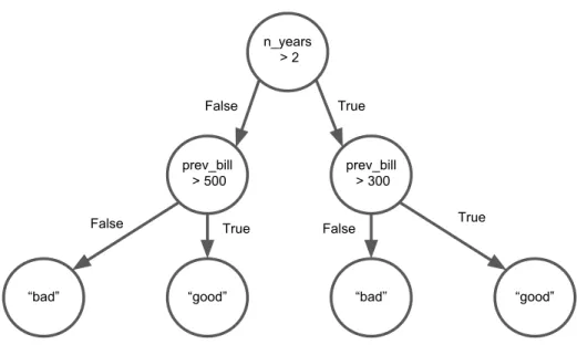
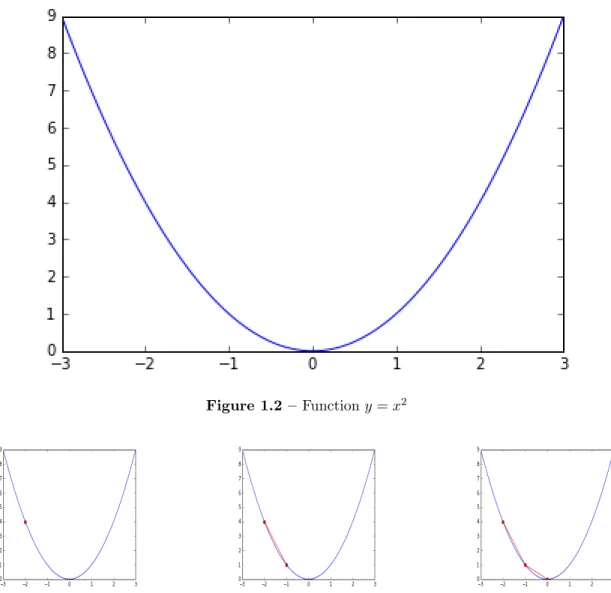
Imagine we wish to find the minimum of a function which follows the curve y = x2 shown in Figure1.2. If we continuously move down the “hill” (down the gradient with respect to x, Figures1.3) we will eventually reach the minimum of the function. Choosing how far to move each time the gradient is calculated is a choice that must be made. We generally call this step size, or learning rate in many gradient based optimizers. The learning rate is the first of many possible hyperparameters, which is a general terminology for settings that cannot be optimized, and must be set beforehand by the algorithm designer or programmer. The choosing of hyperparameters is absolutely critical to the performance of many models, and comprises folk knowledge in diﬀerent fields of machine learning.

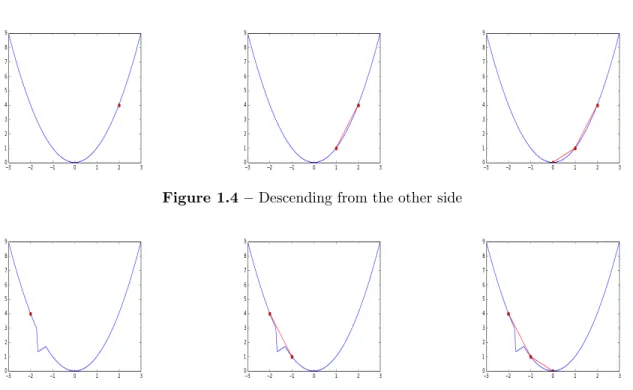
If we instead start on the right as in Figure 1.4, the gradient points the oppo-site direction, and we still move toward the global minimum. The theory behind gradient based optimization for convex (and non-convex) models is a huge field of study (Bottou, 1998), but here we present a simple example explaining the intu-ition behind gradient based optimization. Addintu-itionally, it is easy to see that this type of model can also work for non-convex functions, given the right settings of

(29)

Figure 1.2 – Function y = x2

Figure 1.3 – Moving down the gradient to a minimum

the optimizer.

Figure 1.5 shows a non-convex problem, with a minima near x = −1. It easy to see that with the right step size we would still be able to find the minimum of the function, by stepping directly over the problem region. However, without prior knowledge of where the problem region lies it would be quite diﬃcult to purposefully choose settings that avoid issues. Indeed, there are many diﬀerent techniques used when bridging the gap from convex linear models to non-convex models such as neural networks (LeCun et al., 1998).

(30)

Figure 1.4 – Descending from the other side

Figure 1.5 – Descending non-convex function, by “skipping” the problem region

as in Choromanska et al. (2014) and Dauphin et al. (2014)) in optimization is a problem of current interest as many models are not guaranteed to be convex with respect to all parameters. It is also important to note that we generally optimize L(y, f (x, θ)) with respect to parameters θ. The general intuition of gradient descent as a movement along a surface can be quite useful (Goodfellow,2015).

The process of proceeding from a starting point, or initialization, to some mini-mum of a function by changing parameters θ, whether by gradient descent or some other means, is broadly called learning. Optimization and learning are often used interchangeably in existing literature as well as in this thesis, but there exist meth-ods of learning which are not based on optimization explicitly (Mitchell, 1998).

Deriving the gradients of the cost with respect to the parameters θ in a linear model (θ being the combined elements of W and b) is a straightforward applica-tion of calculus and there are many resources for such derivaapplica-tions such as Bishop

(2006) andHastie et al.(2001). Computational toolkits for gradient based machine learning such as Bastien et al. (2012) and Abadi et al. (2015) often use methods to automatically calculate the gradients of many common functions either symbol-ically or numersymbol-ically, and are a crucial piece of implementing more complex models such as neural networks.

(31)

An additional note is that optimization generally becomes more diﬃcult as the number of parameters grows, also known as the “curse of dimensionality” in

Bellman (1957). There exist models with thousands or millions of parameters and optimizing such models can be quite diﬃcult especially in non-convex settings. Finding clever ways to reduce the number of necessary parameters for a model can often greatly improve performance on a given task, and we will discuss some techniques for parameter sharing in later sections.

1.5.2 Stochastic, Minibatch, and Batch Gradient Descent

In the framework of gradient based optimization, we have additional choices on how to actually implement the optimization algorithm. Theoretical guarantees on convergence speed in the case of convex functions (Bottou,1998) often lean toward taking a single example xi, calculating the gradient of the cost L(xi) with respect to

parameters θ, then performing an update θt= θt−1− ηgradθ(L(xi)), with learning

rate η > 0 and previous parameter settings θt−1. This parameter update rule is

commonly known as stochastic gradient descent, or SGD (Bottou, 1998).

By calculating the average cost with respect to several samples (sometimes called a minibatch), and then calculating the updates to θ, we can smooth out issues related to badly modeling single samples, while the dataset as a whole is well modeled. In the extreme case, we can calculate the loss over the entire dataset (so called batch gradient descent ), and then update parameters, θ.

In general the choice of which type of gradient descent (stochastic, minibatch, or batch) to use is yet another hyperparameter. Many practitioners choose to use minibatch gradient descent due to the ability to increase or decrease the number of samples in the minibatch, allowing flexibility when modeling new datasets, while also controlling practical issues such as memory usage and data access times. There also exist more advanced gradient based optimizers and adaptations such as dis-cussed in Kingma and Ba (2015), Dauphin et al. (2014), Sutskever et al. (2013),

Bengio et al. (2013),Zeiler (2012), Hinton(2012), and Duchi et al.(2011).

1.5.3 Regularization

In addition to a cost assumption, it is common to add constraints on the type of solution desired, in the form of an additional regularizer, RG. In the framework

(32)

of empirical risk minimization, this results in a modified formulation as seen in Equation 1.49. ER(θ) = 1 l l ∑ i=1 L(yi, f (xi, θ)) + RG(θ) (1.49)

The case of weight norm penalties is discussed in Vapnik (1991), and is a com-mon addition to many models to reduce numerical issues and improve training sta-bility. In the specific case of linear models the addition of weight norm constraints results in the well known LASSO (L1), Ridge (L2), and ElasticNet estimators (L1 and L2) as demonstrated inBishop(2006). The relative weighting between the loss, L, and the regularizer, RG, is another important hyperparameter. It is typically chosen by trial and error on a subset of the full dataset.

1.6 Basic Learning Algorithms

1.6.1 Linear Regression

Combining the linear model q(x) = W x + b with the mean squared error loss results in the following formulation, where yi is the paired y coordinate for the

sample xi. L(x) = 1 l l ∑ i=0 (yi− q(xi))2 (1.50) L(x) = 1 l l ∑ i=0 (yi− (W xi+ b))2 (1.51)

1.6.2 Logistic Regression

Bernoulli cross-entropy with q(x) = W x + b, is a potentially simple model for classification, but there is one major problem. The default output of q(x) is unbounded, but for the Bernoulli cross-entropy cost to work, the output of q(x) must be bounded between 0 and 1. One way to bound the output is to introduce a non-linear activation to squash the outputs into the correct range. The sigmoid

(33)

Figure 1.6 – Sigmoid function sigm(x) = _1+exp1 _−x

(also known as the logistic function), shown in Figure 1.6, is the ideal function to enforce the bounds.

Denoting the sigmoid function as sigm(x), we modify the model q(x) = sigm(W x+ b). Plugging into the Bernoulli cross-entropy, we see the classic formulation for lo-gistic regression. Lolo-gistic regression is very closely related to the perceptron which forms the foundations of modern neural networks (Rosenblatt, 1958).

L(x) = 1 l l ∑ i=0 yilog q(xi) (1.52) L(x) = 1 l l ∑ i=0 yilog sigm(W xi+ b) (1.53)

1.6.3 Multinomial Logistic Regression

Using the familiar linear model q(x) = W x+b with the categorical cross-entropy loss has similar problems as two-class logistic regression. Once again, it is necessary to bound the outputs between 0 and 1 in order for the loss function to work. In

(34)

the multiclass case, the softmax activation function, denoted by s(x) and shown in Equation 1.54, is the best choice (Bishop, 2006).

s(x) = exp

xj

∑k

i=0expxk

f or j = 0· · · k (1.54) We can define the full loss for multinomial logistic regression using the correct class from the target data, c, combined with q(x) = s(W x + b).

L(x) = 1 l l ∑ i=0 yi[c] log q(xi)[c] (1.55) L(x) = 1 l l ∑ i=0 yi[c] log s(W xi+ b)[c] (1.56)

1.7 Neural Networks

Next, we might consider ways to add more parameters to these kinds of models. One way is to create more input features, m, so that the matrix W (shape (m, d)) becomes larger. Next, we might try having two matrices, W1 and W2, of size (m,

d1) and (d1, d), so that the model becomes q(x) = W2W1x + b. Unfortunately this

cannot increase the number of parameters (sometimes called capacity), because the composition of linear transforms can still be represented by a single transform (Ogus, 2007). When holding the feature size constant with a required output size dependent on the cost and targets, there seems to be no way to increase the number of parameters.

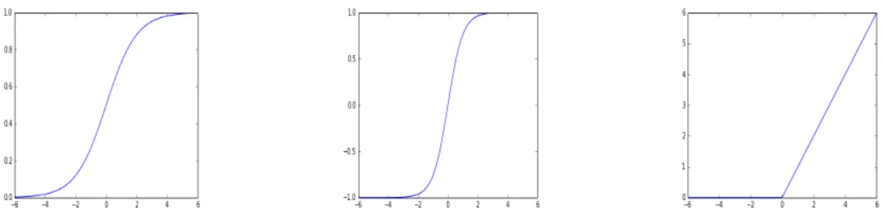
Figure 1.7 – Graphs demonstrating nonlinear functions from left to right: Sigmoid (_1+exp1 _−x), tanh (1_1+exp−exp−2x−2x), and rectified linear (0 if x < 0 else x)

(35)

One way to prevent the linear transformations from combining is to introduce a non-linearity, such as a sigmoid, hyperbolic tangent, or rectified linear functions. Examples of each can be seen in Figure 1.7. The resulting model may look some-thing like q(x) = W1sigm(W2x)+b, or for two functions f () and g(), q(x) = f (g(x)).

To calculate the gradients with respect to the parameters associated with f () and g(), the standard chain rule of calculus can be used (Finney et al., 2003; Rumel-hart et al., 1986). This stacking of multiple parameterized non-linear functions (called layers) with a loss function forms a basic neural network sometimes called a multilayer perceptron, or MLP is shown inRumelhart et al.(1986). These linear transforms with a non-linearity applied afterward are commonly called feedforward layers. The loose assumption of feedforward layers in the MLP is roughly “every-thing to every“every-thing”, or that the value at xi[n] depends on all xi[̸=n], meaning the

function captures f (xi[0]...xi[n]) for all feature indices n.

1.8 Networks Which Exploit Structure

The models we have talked about so far share parameters over dataset sam-ples, roughly based on the assumption that dataset examples are drawn from some underlying data distribution or have some common information which is shared over examples. There are additional assumptions we can make about the struc-ture of each example, which often allows for a further reduction in the number of parameters. Parameter sharing is one of the most powerful tools in the arsenal of practitioners, and finding new ways to share parameters on a dataset can often result in much better solutions than previous attempts.

1.8.1 Convolutional Networks

The basic motivation for convolutional neural networks, first seen inFukushima

(1980), centers around the concept of shared statistics. Namely, we believe that in some types of data (such as images) there are statistics which are shared over the data sample. This is commonly exploited in the form of cutting images into smaller “patches”, then processing patches, rather than whole images Coates et al. (2012). One common assumption is that images are made from a hierarchy of shape types,

(36)

starting from edges and blobs which are then further combined into more compli-cated shapes. If we wanted to craft an edge detector, it would be a bit strange to choose a number of parameters that is the same size as the image. This is because edge detection is fundamentally local. Rather we can use something much smaller such as a 3 by 3 filter which is repeatedly dotted and shifted over the whole image

Sobel and Feldman (1968). This repeated “dot and shift” procedure is also known as convolution, and is a common operation in image processing. Convolution with handcrafted filters has formed the core of signal and image processing for many years, but by using the right layers in a neural network, we can create learned filters which start randomly and are trained by gradient descent. These filters can be optimized toward a specific goal, combined with the right cost and task such as image classification (Krizhevsky et al., 2012a), audio modeling (Dieleman and Schrauwen, 2014), or text classification [cite convnet sentiment]. In addition we can stack these layers on top of each other with the goal of learning a set of hi-erarchical filters such that for images it first detects edges, then groups of edges, and eventually detectors for complex objects Yosinski et al. (2015). A similar in-tuition of first matching small features, then hierarchical groupings of features as the network gets deeper, also holds for other types of inputs. The details of convo-lutional networks can be found in many places such as Fukushima(1980), LeCun et al. (1997), Krizhevsky et al. (2012a), Goodfellow et al. (2016), Sermanet et al.

(2014), Simonyan and Zisserman (2015), Szegedy et al. (2014). Sharing weights over dimensions of data because of similar statistics provides an important way to improve the performance of neural networks. We use this technique heavily in modern research, and the papers included in Chapters 2.2 and 3 are no exception. One key piece of convolutional networks is the assumption of independence. In a given layer, each local filter application is assumed to be independent of the other filter applications. As such the filters at each layer can be calculated in parallel, allowing for eﬃcient computation on modern computers and parallel processing devices. We can roughly say that convolutional networks model the assumption f (x_i[j₋k

2]...xi[j+

k

2]) where k is the convolutional filter size, and j is the current filter

position. Convolutional models capture the full relationship between all features f (xi[0]...xi[n]) only after stacking many convolutional layers, eﬀectively partitioning

the space over depth so that nearby interactions have highly similar paths through the network while more distant features have more disjoint paths (Dinh, 2016). If

(37)

the sample xi is multi-dimensional such as an image, the independence

assump-tion may also have multiple dimensions depending on the size of the filter in each dimension. In the extreme case of filter size equal to sample size, a convolutional layer is equivalent to a feedforward layer with the same nonlinearity.

1.8.2 Recurrent Neural Networks

Recurrent neural networks are another way of sharing parameters, as seen in

Jordan(1986) andElman(1990). Unlike the previous example of convolutional neu-ral networks, recurrent neuneu-ral networks make no independence assumptions within the same layer. Instead, it factorizes the joint model f (xi[0]...xi[n]) as a sequence of

conditional functions f (xi[0]), f (xi[1]|xi[0]), f (xi[2]|xi[1], xi[0]), f (xi[3]|xi[2], xi[1], xi[0])

... up to f (xi[n]|xi[n−1], ..., xi[0]). In standard training (combined with the

cor-rect cost) these conditional functions form probability distributions, so that we eﬀectively factorize the joint probability distribution p(xi[0]...xi[n]) as a product of

conditional distributions p(xi[0])∗ p(xi[1]|xi[0])...p(xi[n]|xi[n−1]...xi[0]) (Larochelle and

Murray, 2011a). The general idea of recurrent neural networks is that the out-put for a specific position k can be thought of as a function of the current inout-put xi[k] and some previous information (often called the hidden state) hk−1 which

attempts to compress all previous history xi[0...k−1]. This results in a function

hk = f (r(xi[k]) + hk−1), with input feature model r() and hidden state h. By

starting this process recursively, and allowing the hidden state to be shared over all steps k in 0...n, this results in the factorization described above. In addition, the function f () and hidden state processing can have memory, error correction, or a host of diﬀerent useful computational blocks. Details for specific recurrent neural networks will be found in subsequent chapters, but a general overview of the concept and introductions to specific architectures can be found in Hochreiter and Schmidhuber(1997),Cho et al. (2014),Goodfellow et al. (2016),Graves et al.

(38)

1.9 Structured Prediction

If the chosen model (and associated cost) is more advanced, we may use it to predict multiple things about a single sample. Some examples include classifying each pixel in an image (such as road, car, tree) as in Eigen and Fergus (2015) or notes in a piece of music as in Eck and Schmidhuber (2002) and Boulanger-Lewandowski et al. (2012a). Standard prediction problems (such as classification) can be thought of as learning a mapping function f (yi|xi), where xi is a feature

vector of some kind, and yi is a single target for that mapping. A simple problem

dealing with structured prediction might involve prediction of multiple targets for each sample, f (yi[0]...yi[l]|xi). Many other problems have further knowledge which

can be mined or described about the relationship between targets. This allows var-ious breakdowns of the cost function into related subproblems that may (or may not) share parameters. These types of problems are common in natural language processing and speech recognition. Much study in modern research is focused on better ways of handling so called structured output tasks, and incorporating prior knowledge in the output structure can provide massive improvements on a given task. There are also ways to learn one to many mappings by outputting the param-eters for mixture densitiesBishop (1994), but we leave this for further exploration in subsequent chapters. In the next chapter we discuss a method for structured prediction of handwriting and audio sequences, called a variational recurrent neural network, or VRNN.

(39)

2

A Recurrent Latent

Variable Model For

Sequential Data

2.1 Prologue to the Article

A Recurrent Latent Variable Model for Sequential Data. Junyoung Chung, Kyle Kastner, Laurent Dinh, Kratarth Goel, Aaron Courville, Yoshua Ben-gio.

Published in Advances in Neural Information Processing Systems 28, NIPS 2015.

Personal Contribution. The idea for this form of model with recurrent latent variables was conceived by Yoshua and Junyoung with involvement from Laurent, Aaron, and I in a brainstorming session during the MILA speech synthesis group meeting. Junyoung developed a prototype that showed the idea working and we soon started running experiments on various datasets. Laurent formalized the mathematical side of the model, with Junyoung reviewing and input from Yoshua and Aaron. Later, Kratarth joined Junyoung and I in running additional experi-ments. I handled dataset issues around the handwriting dataset and assisted Juny-oung with speech experiments. Laurent developed the visualization for the change in latent states over the sequence. We all assisted in writing the final paper. I pro-vided content in the background, datasets, and analysis sections of the paper. My research role centered around assisting in debugging the model and code, organizing test datasets, running experiments, and analyzing generated results.

Aﬃliations

Junyoung Chung, MILA, Département d’Informatique et de Recherche Op´ era-tionnelle, Université de Montréal

Kyle Kastner, MILA, Département d’Informatique et de Recherche Op´ era-tionnelle, Université de Montréal

Laurent Dinh, MILA, Département d’Informatique et de Recherche Op´ era-tionnelle, Université de Montréal

(40)

Kratarth Goel, MILA, Département d’Informatique et de Recherche Op´ era-tionnelle, Université de Montréal

Aaron Courville, MILA, Département d’Informatique et de Recherche Op´ era-tionnelle, Université de Montréal

Yoshua Bengio, MILA, Département d’Informatique et de Recherche Op´ era-tionnelle, Université de Montréal, CIFAR Senior Fellow

Funding We acknowledge the support of the following agencies for research funding and computing support: Ubisoft, Nuance Foundation, NSERC, Calcul Quebec, Compute Canada, the Canada Research Chairs and CIFAR.

2.2 Abstract

In this paper, we explore the inclusion of latent random variables into the hidden state of a recurrent neural network (RNN) by combining the elements of the variational autoencoder. We argue that through the use of high-level latent random variables, the variational RNN (VRNN)1can model the kind of variability observed in highly structured sequential data such as natural speech. We empirically evaluate the proposed model against other related sequential models on four speech datasets and one handwriting dataset. Our results show the important roles that latent random variables can play in the RNN dynamics.

2.3 Introduction

Learning generative models of sequences is a long-standing machine learning challenge and historically the domain of dynamic Bayesian networks (DBNs) such as hidden Markov models (HMMs) and Kalman filters. The dominance of DBN-based approaches has been recently overturned by a resurgence of interest in recur-rent neural network (RNN) based approaches. An RNN is a special type of neural network that is able to handle both variable-length input and output. By training

(41)

an RNN to predict the next output in a sequence, given all previous outputs, it can be used to model joint probability distribution over sequences.

Both RNNs and DBNs consist of two parts: (1) a transition function that determines the evolution of the internal hidden state, and (2) a mapping from the state to the output. There are, however, a few important diﬀerences between RNNs and DBNs.

DBNs have typically been limited either to relatively simple state transition structures (e.g., linear models in the case of the Kalman filter) or to relatively simple internal state structure (e.g., the HMM state space consists of a single set of mutually exclusive states). RNNs, on the other hand, typically possess both a richly distributed internal state representation and flexible non-linear transition functions. These diﬀerences give RNNs extra expressive power in comparison to DBNs. This expressive power and the ability to train via error backpropagation are the key reasons why RNNs have gained popularity as generative models for highly structured sequential data.

In this paper, we focus on another important difference between DBNs and RNNs. While the hidden state in DBNs is expressed in terms of random variables, the internal transition structure of the standard RNN is entirely deterministic. The only source of randomness or variability in the RNN is found in the condi-tional output probability model. We suggest that this can be an inappropriate way to model the kind of variability observed in highly structured data, such as natural speech, which is characterized by strong and complex dependencies among the output variables at different timesteps. We argue, as have others ( Boulanger-Lewandowski et al., 2012b; Bayer and Osendorfer, 2014), that these complex de-pendencies cannot be modelled efficiently by the output probability models used in standard RNNs, which include either a simple unimodal distribution or a mixture of unimodal distributions.

We propose the use of high-level latent random variables to model the variability observed in the data. In the context of standard neural network models for non-sequential data, the variational autoencoder (VAE) (Kingma and Welling, 2014;

Rezende et al.,2014) oﬀers an interesting combination of highly flexible non-linear mapping between the latent random state and the observed output and eﬀective approximate inference. In this paper, we propose to extend the VAE into a re-current framework for modelling high-dimensional sequences. The VAE can model

Structured prediction and generative modeling using neural networks

Résumé

Summary

Contents

List of Figures

List of Tables

List of Abbreviations

Acknowledgments

1

Introduction

1.1

Overview

1.2

Types of Learning

1.3

A Formal Definition of Learning

1.4

Losses

1.4.1

Relationship between KLD and MLE

1.4.2

Bernoulli Cross-entropy

1.4.3

Categorical Cross-entropy

1.4.4

Gaussian Negative Log-Likelihood

1.4.5

Mean Squared Error

1.5

A Basic Model

1.5.1

Gradient Based Optimization

1.5.2

Stochastic, Minibatch, and Batch Gradient Descent

1.5.3

Regularization

1.6

Basic Learning Algorithms

1.6.1

Linear Regression

1.6.2

Logistic Regression

1.6.3

Multinomial Logistic Regression

1.7

Neural Networks

1.8

Networks Which Exploit Structure

1.8.1

Convolutional Networks

1.8.2

Recurrent Neural Networks

1.9