HAL Id: cea-02339097
https://hal-cea.archives-ouvertes.fr/cea-02339097v2
Submitted on 5 Mar 2020
HAL is a multi-disciplinary open access
archive for the deposit and dissemination of
sci-entific research documents, whether they are
pub-lished or not. The documents may come from
teaching and research institutions in France or
abroad, or from public or private research centers.
L’archive ouverte pluridisciplinaire HAL, est
destinée au dépôt et à la diffusion de documents
scientifiques de niveau recherche, publiés ou non,
émanant des établissements d’enseignement et de
recherche français ou étrangers, des laboratoires
publics ou privés.
Comparison of MAVRIC/Monaco and TRIPOLI-4
Simulations of the LLNL Pulsed Spheres Benchmark
Experiments
T. Miller, E. Le Menedeu, D. Mancusi, A. Zoia
To cite this version:
T. Miller, E. Le Menedeu, D. Mancusi, A. Zoia. Comparison of MAVRIC/Monaco and
TRIPOLI-4 Simulations of the LLNL Pulsed Spheres Benchmark Experiments. RPSD 2018 - 20th Topical
Meeting of the Radiation Protection and Shielding Division, Aug 2018, Santa Fe, United States.
�cea-02339097v2�
ANS RPSD 2018 - 20th Topical Meeting of the Radiation Protection & Shielding Division of ANS
Santa Fe, NM, August 26 – 31, 2018, on CD-ROM, American Nuclear Society, LaGrange Park, IL (2018)
†TRIPOLI-4® is a registered trademark of CEA.
COMPARISON OF MAVRIC/MONACO AND TRIPOLI-4® SIMULATIONS OF THE LLNL PULSED SPHERES BENCHMARK EXPERIMENTS
T. M. Miller1, E. Le Ménédeu2, D. Mancusi2, and A. Zoia2
1Oak Ridge National Laboratory, P.O. Box 2008, Oak Ridge, TN, 37831, USA millertm@ornl.gov
2 Den-Service d’études des réacteurs et de mathématiques appliquées (SERMA), CEA, Université Paris-Saclay, F-91191,
Gif-sur-Yvette, France, eve.le-menedeu@cea.fr, davide.mancusi@cea.fr, andrea.zoia@cea.fr
Simulations of the Lawrence Livermore Pulsed Spheres with MAVRIC/Monaco and TRIPOLI-4® are presented. Both codes use ENDF/B-VII.1 cross section data, but TRIPOLI-4® also uses cross section data based on JEFF-3.1.1. The MAVRIC/Monaco simulations were performed with the SCALE 6.2.2 release while the TRIPOLI-4® simulations used an internal development version of the code. For the most part, the simulated and measured neutron counts agree within 30%. Simulated gamma flux data is compared, as well. There are no measured gamma data. The agreement between the simulated gamma flux spectra is often within 10% or less, but there some notable differences, especially when comparing simulations using ENDF/B-VII.1 and JEFF 3.1.1 based cross section data. The comparison of photon simulations suggests that improvements are needed in the cross-section data, cross section processing codes, and/or transport codes and gamma measurement data is needed for experimental validation.
I. INTRODUCTION
The Lawrence Livermore Pulsed Spheres1,2 (LPSs)
benchmark experiments were performed specifically to test new radiation transport codes being developed at the time, but the results continue to provide valuable data today. These benchmark experiment results are also a good test of the total, elastic, and inelastic cross section data. By the middle of 1971, the LPS experiments measured the neutron emission spectra for 17 isotopic, elemental, and compound spherical targets via time-of-flight techniques. These spherical targets varied in thickness from 0.5 to 5 mean free paths (mfp) for 14 MeV neutrons. The source in each measurement was 14 MeV neutrons born from deuterium-tritium (DT) fusion reactions at the center of each sphere. These neutrons were born at times that resulted in a Gaussian distribution, with a mean of 0 ns and full-width-at-half-maximum of 3, 4, 5, or 6 ns. The time-of-flight measurements were made along two different flight paths, 30° and 120°. These angles were measured with respect to the direction of travel of the deuterons. Either a Pilot B plastic or NE213 liquid scintillator was used to measure neutrons at 30°, but only a NE213 liquid scintillator was used for the 120° measurement. Along the 30° flight path, the distance from the DT source to the detector for most of
the measurements was about 765 cm, but a few were around 753 cm. For the 120° flight path, this distance for all the measurements was about 976 cm.
Oak Ridge National Laboratory (ORNL) and the Commissariat à l’Énergie Atomique et aux Énergies Alternatives – Centre de Saclay (CEA-Saclay) performed simulations of the LPS benchmark experiments to add these results to the suite of validation problems of
MAVRIC/Monaco3 and TRIPOLI-4®.4† This paper
presents results for the following spheres: 0.8 mfp Be, 2.9 mfp C, 3.1 mfp N, 0.9 mfp iron, and 2.0 mfp concrete. The benchmark measurement data provided by Wong1 are the
time-dependent neutron count rates at the different detector locations. Simulation results for MAVRIC/Monaco version 6.2.2 and a development version of TRIPOLI-4®, which will become version 11, are compared to the measured data for some of the LPSs. Additionally, the calculated gamma flux spectra on the surface of each LPS are compared. The calculated gamma flux is the integral over all time. In other words, no time and energy cutoffs were used in these simulations other than a 100 keV energy cutoff for the photons, so these spectra may include photons produced after the measurement time of the LPS. Both Monte Carlo codes use cross sections based on ENDF/B-VII.1 for these simulations. However, TRIPOLI-4® results with cross sections based on JEFF-3.1.1 are also presented.
II. COMPUTATIONAL TOOLS AND DATA
The ORNL results contributed to this work were simulated using the MAVRIC sequence in SCALE 6.2.2. The MAVRIC sequence mixes cross sections for the Monaco fixed-source Monte Carlo code, automatically generates variance reduction parameters for Monaco, and executes Monaco. However, the automated variance reduction typically provided by the MAVRIC sequence for the Monaco Monte Carlo code was not used for this analysis, so MAVRIC was simply used to mix cross sections for Monaco and run Monaco. The only variance reduction techniques used for the MAVRIC/Monaco simulations were implicit capture, Russian roulette and splitting, and biasing of the angular source distribution. MAVRIC/Monaco can use multigroup or continuous energy cross sections. For this work the continuous energy
neutron and photon cross sections based on ENDF/B-VII.1 were used (ce_v7.1_endf), which are produced by AMPX5
and provided with SCALE 6.2.2. None of the available thermal scattering data were used because the lowest energy neutrons measured in these benchmark experiments were around 1.7 MeV.1 The lowest temperature cross
section data available with SCALE 6.2.2 are room temperature, 293 K. Some of the material temperatures for the nitrogen simulations are well below room temperature (liquid nitrogen). The correct temperature was set on the material cards in the MAVRIC/Monaco input, which usually results in correctly broadened cross section data for the given temperature. However, since the nitrogen temperature is below room temperature and SCALE will only interpolate the available temperature dependent cross section data—i.e., no extrapolation—the room temperature cross sections are used with temperature corrections for free gas elastic scattering and collision kinematics.
TRIPOLI-4® represents the fourth generation of the production Monte Carlo code for continuous-energy particle transport developed by CEA. The new major version 11 is scheduled for release at the end of 2018. All the TRIPOLI-4® results presented in this paper use a developmental version of TRIPOLI-4® that will become version 11. TRIPOLI-4® can simulate neutrons, photons and the electromagnetic shower, including electrons and positrons. Several variance reduction techniques are available, including a special built-in variance reduction module with an automatic precalculation of the importance function. For the purpose of the LPS calculations, the only variance-reduction techniques used were implicit capture and Russian roulette and splitting. For neutron transport, TRIPOLI-4® can directly use any nuclear data library in ENDF format without any extra treatment step; for the purposes of this paper, calculations were performed using ENDF/B-VII.1 and JEFF-3.1.1. Cross section data at 300K were used for these simulations, and the free gas treatment
was used for all materials. For photon transport, TRIPOLI-4® relies on the cross sections and parameterizations provided by the EPDL97 library.6
III. MODEL DESCRIPTION
This section briefly summarizes the computation models used in these simulations. Most of the information in this section was taken from Wong et al.1 and Plechaty
and Howerton,2 which should be consulted for additional
details.
III.A. Geometry and Materials
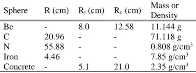
Even though these benchmark experiments are referred to as spheres, some of them are actually spherical shells. Regardless, all of them have either a cylindrical or conical frustum cutout where the source assembly can be placed within the sphere. Some of these cutouts are more complicated, like the C sphere with a cutout that is a combination of a cylinder and conical frustum. A generic two-dimensional schematic of these geometry options is shown in Figure 1. Table I provides numerical values of the dimensions labeled in Figure 1 along with the mass or density of each sphere (depending on which was specified in Wong et al.1). Three of the five LPS simulated for this
work were elemental with naturally occurring isotopic abundances and no reported impurities. The elemental compositions of the fourth and fifth spheres, which were iron and concrete, are provided in Table II.
TABLE I. Sphere dimensions and mass or density.
Sphere R (cm) Ri (cm) Ro (cm) Mass or Density Be - 8.0 12.58 11.144 g C 20.96 - - 71.118 g N 55.88 - - 0.808 g/cm3 Iron 4.46 - - 7.85 g/cm3 Concrete - 5.1 21.0 2.35 g/cm3
Fig. 1a. Example spherical geometry. Fig. 1b. Example spherical shell geometry.
R
Ri
TABLE II. Elemental atom percent of iron and concrete spheres.
Element Iron Concrete Element Iron Concrete Element Iron Concrete
H - 15.1 Al - 3.2 Ca - 3.6
C < 1.2 3.1 Si - 14.9 Ti - < 1.0
O - 55.7 P < 0.7 - Mn < 1.0 < 1.0
Na - 1.3 S < 0.1 - Fe > 97.0 < 1.0
Mg - 1.8 K - < 1.0
Fig. 2. Energy and angular distribution of DT neutrons.
The geometry of the facility surrounding the LPS and source assembly is taken from Bennett and Kiedrowski,7
including the material composition and dimensions of the surrounding room and collimators. This model is very simplistic, but it is adequate for these simulations because neutrons above 1 MeV are the primary interest.
III.B. Source
The source neutrons were provided by DT fusion reactions. The energy and angular distribution of the neutrons used in these simulations are the results of simulations by Marchetti and Hedstorm.8 A plot of the
energy and angular neutron distribution is provided in Figure 2.
The time dependence of the source neutrons was studied by the experimenters and was determined to have a Gaussian shape.1 In all instances, the mean of this Gaussian
is 0 ns. The full-width-at-half-maximums for each measurement are all between 3 and 6 ns.1 Continuous
energy and time-dependent transport were recently implemented in the Monaco Monte Carlo code in SCALE
(version 6.2), but a time-dependent source has not been implemented. Therefore, the source neutrons are all born at 0 ns in the MAVRIC/Monaco simulation, which will obviously affect the results at the earliest measurement times. TRIPOLI-4 is able to fully model the Gaussian time distribution of the source neutrons.
III.C. Tallies
The tally normalization (source strength) needed for these simulations is not provided explicitly. The measured data are provided on a relative basis, counts with the sphere relative to the total number of counts without the sphere, so the explicit source strength is not needed.1 Each
configuration is simulated with the sphere material and with each sphere material replaced by air. The results presented later in this paper use this method to normalize the tallies and divide the results by the widths of the time bins (2 ns). The detector response functions are needed to convert the Monte Carlo tallies to counts in the Pilot B or NE213 scintillators.2 These response functions are plotted
in Figure 3, which have units of counts per fluence (A is the detector area and ε is the efficiency).
10.8 0.60.4 0.20 -0.2-0.4 -0.6-0.8-1 0 0.005 0.01 0.015 0.02 0.025 0.03 0.035 0.04 0.045 0.05 12.8 13 13.2 13.4 13.6 13.8 14 14.2 14.4 14.6 14.8 15 15.2 15.4 15.6 15.8 Co sin e Pr ob ab ilit y Energy (MeV) 0-0.005 0.005-0.01 0.01-0.015 0.015-0.02 0.02-0.025 0.025-0.03 0.03-0.035 0.035-0.04 0.04-0.045 0.045-0.05
Fig. 3. Pilot B and NE213 detector response functions.
The MAVRIC/Monaco neutron tallies for this work use a volumetric region tally. This volumetric region ends up being a ring, or more precisely the segment of a spherical shell. The simplistic geometry of the room surrounding the spheres allows one to take advantage of the symmetry of the tally region. Bennett and Kiedrowski accomplish this via a ring detector.6 MAVRIC/Monaco
does not have a ring detector, so this volumetric region is used instead. The thickness of the region tally is 1 cm along the radius from the source region to the tally region. The distance from the source region to the center of the tally region is the flight path provided in Wong et al.1
Similarly, the tally for the TRIPOLI-4® simulations took advantage of the axial symmetry to maximize collected statistics. Contrary to the MAVRIC/Monaco simulations, the neutron tally was a surface current across a spherical shell with a radius equal to the nominal flight path. The angular acceptance of the tally region was determined by the surrounding concrete collimators; it amounted to about 3° for the 30° beamline and 2.5° for the 120° beamline.
The gamma flux tally in the MAVRIC/Monaco simulations was also a volumetric region tally. The tally volume covered the entire surface of each sphere, excluding the cutout for the source assembly. The thickness of this tally region in the radial direction was 1 mm. No response function was applied to the gamma flux tally. The gamma flux tally is energy dependent, integrating over all time, but a cutoff energy of 100 keV was applied. No neutron cutoff energy was applied in the simulations to allow for low energy neutrons to be absorbed and create capture gammas.
The TRIPOLI-4® photon score was taken to be the flux integrated on the outer surface of each sphere, excluding the cutout for the source assembly. The same energy cutoffs were applied as those applied in the MAVRIC/Monaco simulations.
IV. RESULTS
The following subsections present the measured LPS data and the results of the MAVRIC/Monaco and TRIPOLI-4® simulations. No gamma data were measured during the LPS experiments, but the gamma flux on the surface of each sphere was calculated, and these results are also presented in the following subsections. The ratio results presented for the gamma flux data are the MAVRIC/Monaco ENDF/B-VII.1 and TRIPOLI-4® JEFF-3.1.1 results relative to the TRIPOLI-4® ENDF/B VII.1 results. For all plotted data, the error bars represent the 1-sigma uncertainty.
IV.A. Beryllium Sphere, 0.8 MFP, 30°
Neutron counts for the 0.8 mfp Be sphere were only reported at 30°. Figure 4 compares the measured and calculated neutron data, and Figure 5 compares the calculated gamma fluxes on the surface of the sphere.
IV.B. Carbon Sphere, 2.9 MFP, 30° and 120°
Neutron counts were measured at two angles, 30° and 120°, for the 2.9 mfp C sphere. Figure 6 compares the measured and calculated neutron data, and Figure 7 compares the calculated gamma fluxes on the surface of the sphere.
IV.C. Nitrogen Sphere, 3.1 MFP, 30°
Neutron counts for the 3.1 mfp (liquid) N sphere were only reported at 30°. Figure 8 compares the measured and calculated neutron data, and Figure 9 compares the calculated gamma fluxes on the surface of the sphere.
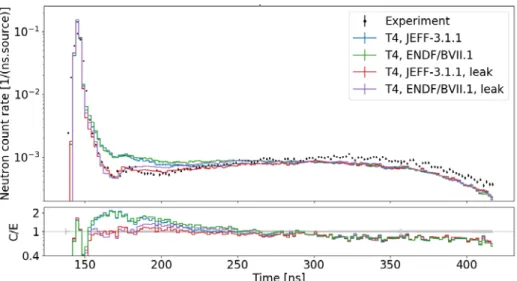
IV.D. Iron Sphere, 0.9 MFP, 30° and 120°
Neutron counts were measured at two angles, 30° and 120°, for the 0.9 mfp iron sphere. Figure 10 compares the measured and calculated neutron data, and Figure 11 compares the calculated gamma fluxes on the surface of the sphere. There is a dramatic difference in the calculated gamma fluxes between 10 and 15 MeV when comparing the simulations with ENDF/B-VII.1 and JEFF-3.1.1 data.
The agreement between the measured and simulated neutron data is always dependent on the collimator material surrounding the detector. However, for the spheres considered in this paper, excluding the iron, the impact of the collimator material is relatively small. In this paper, the collimator model was taken from Bennett and Kiedrowski,7
which is simplified compared to the brief description in Wong et al.1 Neither reference provides complete details.
Models and results related to Bennett and Kiedrowski7
ultimately ignore the collimator by setting the neutron importance to zero in the collimator geometry cells, which removes all contributions due to scattering in the collimator. The original MAVRIC/Monaco and TRIPOLI-4® simulations in this paper do not ignore the collimator, so the results in Figure 10 include neutrons scattered in concrete surrounding the detectors. For all the spheres
except iron, this contribution is negligible. The iron sphere simulations were repeated to remove the neutrons scattered in the collimator, and the results for TRIPOLI-4® are shown in Figure 12. Better agreement can be observed in the simulated data at around 175 and 225 ns for the 30° and 120° angles, respectively. In these additional TRIPOLI-4® simulations, a leakage boundary condition was applied to the collimator cells, so particles that entered the collimator cells were treated as though they leaked from the system. The results shown in Figure 12 with this treatment are labeled “leak.” The MAVRIC/Monaco simulations were also repeated, but with the collimator material replaced by a void. This produced results similar to the TRIPOLI-4® results with the leakage boundary condition.
IV.E. Concrete Sphere, 2.0 MFP, 120°
Neutron counts for the 2.0 mfp concrete sphere were only reported at 120°. Figure 13 compares the measured and calculated neutron data, and Figure 14 compares the calculated gamma fluxes on the surface of the sphere. A peak is observed in the measured data at around 435 ns that is not duplicated in any of the transport simulations.
The measurement data in Wong et al.1 is reported in
2 ns time bins on a per ns basis. For the concrete sphere, there is a missing data point. The missing data point is for the time bin between 312 and 314 ns. After an initial glance at this data, one might assume that between 310 and 316 ns for the concrete sphere, there are two 3 ns time bins rather than three 2 ns time bins. The reported measurement data also includes the integral number of counts over the measurement time. Further investigation finds that the integral data is always consistent with 2 ns time bins, which means that no measurement data are reported between 312 and 314 ns. The TRIPOLI-4® simulations were set up to correctly address this by always using 2 ns time bins. The MAVRIC/Monaco simulations were not set up in this manner, but they have been adjusted to correct for this. This missing measured data point is reflected in the C/E portion of Figure 13 by a small gap in the ratio data. This gap shows the time during which the missing data point should be located, and it also prevents division by zero because the TRIPOLI-4® simulation has more data points than the measurement.
Fig. 5. Gamma flux on surface of Be sphere.
Fig. 6a. Neutron counts at 30° with C sphere.
Fig. 7. Gamma flux on surface of C sphere.
Fig. 8. Neutron counts at 30° with N sphere.
Fig. 10a. Neutron counts at 30° with iron sphere.
Fig. 10b. Neutron counts at 120° with iron sphere.
Fig. 12a. Neutron counts at 30° with iron sphere – no collimator contribution.
Fig. 12b. Neutron counts at 120° with iron sphere – no collimator contribution.
Fig. 14. Gamma flux on surface of concrete sphere. V. SUMMARY AND CONCLUSIONS
V.A. Measured and Simulated Neutron Counts
Comparing the simulated neutron counts to the measured counts, the results for the Be, C, and N spheres are good in the context of a shielding or fixed-source benchmark. In general, the agreement is within ±30% for these spheres outside of the peak at the earliest times for uncollided neutrons. Even though MAVRIC/Monaco was unable to simulate the time dependence of the DT neutron source, the results do not appear to suffer much.
The worst differences between the simulated and measured neutron counts for the iron sphere shown in Figure 10 were addressed by removing contributions from the collimator, as illustrated in Figure 12. Like Be, C, and N, the agreement between the simulations and measurements for the iron sphere is mostly within ±30% outside the uncollided peak, with the contributions from the collimators removed.
Like the other spheres, most of the simulated concrete results are within ±30% of the measured data outside the uncollided peak. The peak at around 435 ns in the measured data is not observed in any of the simulated data. An MCNP6.2 simulation with ENDF/B-VII.1 data was performed, and it also did not produce a peak at around 435 ns. The authors assume that the measured concrete data are correct, even though there is already one other known anomaly in which data between 312 and 314 ns are missing. Therefore, it is thought that there is some missing reaction data in the ENDF/B-VII.1 and JEFF 3.1.1 evaluated nuclear data. Additional benchmark quality measurement data are needed to further evaluate this possibility. However, another plausible explanation, assuming the measured data are correct, is that the actual isotopic composition of the concrete sphere is not exactly known. When considering the other measured data
presented in this paper, it is noted that the C sphere produces two peaks between 225 and 325 ns and another peak at about 435 ns along the 120° angle. If the C atom percent in Table II for concrete is smaller than the actual value (there are known concrete compositions with larger C atom percentages), then the simulated neutron counts around 435 ns might be too low.
The neutron simulation results with
MAVRIC/Monaco and TRIPOLI-4® using ENDF/B-VII.1 and JEFF 3.1.1 cross section data are not in perfect agreement with each other but are fairly consistent. The differences between the simulated and measured neutron data are bigger than between the different simulated neutron data, so one cannot say that one cross section data set performed dramatically different from the other. At this point additional benchmark measurement data is needed. Better documentation of the materials and dimensions could eliminate issues like uncertainty due to the collimator seen with the iron sphere, and better source characterization could eliminate the differences observed at early times between the measured and simulated uncollided neutron peak. Finally, it would also be helpful if a time-dependent source was implemented in Monaco.
V.B. Simulated Photon Fluxes
Comparing the MAVRIC/Monaco and TRIPOLI-4® simulated photon fluxes on the surface of each sphere, many of the results are very good in the context of a shielding benchmark. This means the agreement is within ±10% or better, outside of some statistical uncertainties at high energies. However, there are a few exceptions, which will be discussed next. Recall that the TRIPOLI-4® results presented in this paper were produced by a development version that will become version 11.
For the Be sphere, the agreement is very good down to 5 MeV when both codes use cross sections based on
ENDF/B-VII.1, but below 5 MeV there clearly is a bias (nearly a factor of 2). This bias is eliminated when comparing TRIPOLI-4® simulations with ENDF/B-VII.1 and JEFF 3.1.1 based cross sections, but differences above 11 MeV appear. The differences above 11 MeV are likely due to differences in the ENDF and JEFF cross section data (there are differences like this with other spheres). The bias below 5 MeV needs further investigation, but it appears this is due to an issue with MAVRIC/Monaco or its cross sections.
For the liquid N sphere, there appears to be some differences in the photopeaks between 2.5 and 5 MeV when only ENDF/B-VII.1 based cross sections are used. As with the Be sphere, there are differences between ENDF and JEFF above 11 MeV along with statistical noise.
When ENDF/B-VII.1 based cross sections are used, the agreement for the iron sphere is very good. The introduction of the JEFF 3.1.1 cross sections produces some differences below 3 MeV and above 11 MeV. The differences above 11 MeV are similar to the Be and N spheres.
The simulated photon fluxes for the concrete sphere are very similar regardless of which code or cross section data set was used. The agreement is very good except for some photopeaks between 5 and 7.5 MeV. There are also differences above 12.5 MeV, some of which is statistical noise. However, for the simulations comparing TRIPOLI-4® with ENDF/B-VII.1 and JEFF 3.1.1 based cross sections there appears to be a meaningful difference.
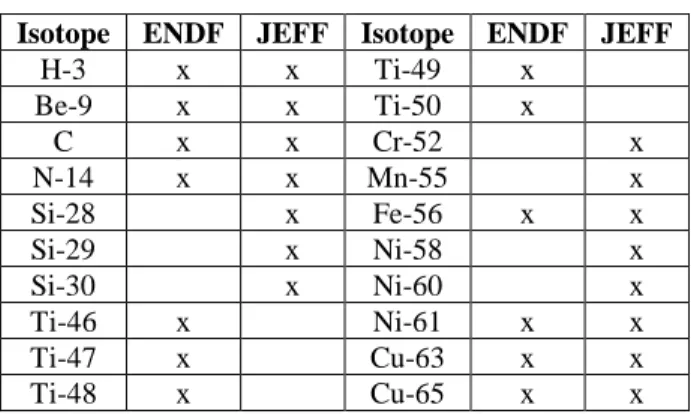
The simulations of gamma flux spectra on the surface of the N, iron, and concrete spheres all seem to produce meaningfully different results when using ENDF/B-VII.1 cross sections as compared to JEFF 3.1.1 cross sections. These differences in the gamma spectra are in part due to differences in gamma production data between the ENDF/B-VII.1 and JEFF 3.1.1 data sets. Table III lists 20 elements and isotopes included in the LPS models and indicates which cross section data sets are missing gamma production data for one or more neutron interaction for these isotopes (x indicates missing data). All the remaining isotopes in the LPS models have complete sets of gamma production data. The data in Table III is based on the TRIPOLI-4® simulations, which notifies the user when gamma production data is missing for one or more specific neutron interaction. MAVRIC/Monaco and MCNP only notify the user if there is no gamma production data at all. If gamma production data is missing from both datasets for an isotope that is less interesting than if gamma production data is available in one data set and not the other. This is because only simulations are considered in this paper rather than comparing simulations and measurements. For the N sphere, the steel container surrounding the liquid N has Si, Cr, Mn, and Ni, which all have isotopes in JEFF 3.1.1 that are missing some gamma production data that are available
in ENDF/B-VII.1. These isotopes make up a large atom fraction of the steel container, but a small fraction of the overall N sphere model. The iron sphere contains Mn, which is also missing gamma production data in JEFF 3.1.1, but Mn is only 1% of the iron sphere. Finally, the concrete sphere contains Si, Ti, and Mn. The JEFF 3.1.1 data set is missing gamma production data for Si and Mn while ENDF/B-VII.1 is missing gamma production data for Ti.
TABLE III. Missing gamma production data. Isotope ENDF JEFF Isotope ENDF JEFF
H-3 x x Ti-49 x Be-9 x x Ti-50 x C x x Cr-52 x N-14 x x Mn-55 x Si-28 x Fe-56 x x Si-29 x Ni-58 x Si-30 x Ni-60 x Ti-46 x Ni-61 x x Ti-47 x Cu-63 x x Ti-48 x Cu-65 x x
Work is needed to improve the agreement between the gamma simulation results. There is clearly some gamma production data that require improvements in the evaluated data, but the cross-section processing codes and the radiation transport codes may need some improvements as well. Separating some of the aspects of these gamma simulations would simplify the investigation. For example, the gamma production due to neutron interactions in the LPSs— the secondary gamma source—can be tallied and compared. Then that secondary gamma source can be transported, and the flux results on the surface of the sphere can be compared. This would reveal whether there are major differences in the gamma production of the neutron cross sections, the interaction cross sections of the gammas themselves, or both. Finally, evaluating the performance of the gamma cross section data would benefit from additional gamma measurement data.
ACKNOWLEDGMENTS
The TRIPOLI-4® developers gratefully acknowledge partial financial support from Électricité de France (EDF).
REFERENCES
1. C. WONG et al., Livermore Pulsed Sphere Program: Program Summary through July 1971, UCRL-51144, Rev. 1, Lawrence Livermore Laboratory (1972). 2. E. PLECHATY and R. HOWERTON, Calculational
Models for LLL Pulsed Spheres, UCID-16372, Lawrence Livermore Laboratory (1973).
3. B. T. REARDEN and M. A. JESSEE, Eds., SCALE Code System, ORNL/TM-2005/39, Version 6.2.2, Oak Ridge National Laboratory (2017).
4. TRIPOLI-4® Project Team, “TRIPOLI-4® CEA, EDF, and AREVA reference Monte Carlo code,” Ann. Nucl. Energy, 82, 151 (2015).
5. D. WIARDA, et. al., AMPX-6: A Modular Code System for Processing ENDF/B Evaluations, ORNL/TM-2016/43, Oak Ridge National Laboratory (2016).
6. D. E. CULLEN, J. H. HUBBELL and L. KISSEL, EPDL97: The Evaluated Photon Data Library ‘97 Version, UCRL-50400 Vol. 6, Rev. 5., Lawrence Livermore National Laboratory (1997).
7. A. S. BENNETT and B. C. KIEDROWSKI, Revisiting the MCNP Shielding Validation Suite, LA-UR-11-04540, Los Alamos National Laboratory (2011). 8. A. MARCHETTI and G. HEDSTORM, New Monte
Carlo Simulations of the LLNL Pulsed-Sphere
Experiments, UCRL-ID-131461, Lawrence