A New Cascade Model for the Hierarchical Joint Classification of Multitemporal and Multiresolution Remote Sensing Data

HAL Id: hal-01308039

https://hal.inria.fr/hal-01308039

Submitted on 27 Apr 2016

HAL is a multi-disciplinary open access archive for the deposit and dissemination of sci-entific research documents, whether they are pub-lished or not. The documents may come from teaching and research institutions in France or abroad, or from public or private research centers.

L’archive ouverte pluridisciplinaire HAL, est destinée au dépôt et à la diffusion de documents scientifiques de niveau recherche, publiés ou non, émanant des établissements d’enseignement et de recherche français ou étrangers, des laboratoires publics ou privés.

Classification of Multitemporal and Multiresolution

Remote Sensing Data

Ihsen Hedhli, Gabriele Moser, Josiane Zerubia, Sebastiano Serpico

To cite this version:

Ihsen Hedhli, Gabriele Moser, Josiane Zerubia, Sebastiano Serpico. A New Cascade Model for the Hierarchical Joint Classification of Multitemporal and Multiresolution Remote Sensing Data . IEEE Transactions on Geoscience and Remote Sensing, Institute of Electrical and Electronics Engineers, 2016, 54 (11), pp.6333 - 6348. �hal-01308039�

1 Ihsen HEDHLI Student Member, IEEE, Gabriele MOSER, Senior Member, IEEE,

Josiane ZERUBIA, Fellow, IEEE, and Sebastiano B. SERPICO, Fellow, IEEE

Abstract—In this paper, we propose a novel method for the joint classification of both multidate and multiresolution remote sensing imagery, which represents an important and relatively unexplored classification problem. The proposed classifier is based on an explicit hierarchical graph-based model that is sufficiently flexible to address co-registered time series of images collected at different spatial resolutions.

Within this framework, a novel element of the proposed approach is the use of multiple quad-trees in cascade, each associated with the images available at each observation date in the considered time series. For each date, the input images are inserted in a hierarchical structure on the basis of their resolutions, whereas missing levels are filled in with wavelet transforms of the images embedded in finer-resolution levels. This approach is aimed at both exploiting multiscale information, which is known to play a crucial role in high resolution image analysis, and supporting input images acquired at different resolutions in the input time series. The experimental results are shown for multitemporal and multiresolution optical data.

Index Terms— Satellite image time series, multitemporal classification, hierarchical

multiresolution Markov random fields.

A New Cascade Model for the Hierarchical Joint

Classification of Multitemporal and Multiresolution

2

I. INTRODUCTION

The capabilities to monitor the Earth’s surface, notably in urban and built-up areas, for environmental disasters such as floods or earthquakes and to assess the ground effects and damage of such events play important roles in multiple social, economic, and human viewpoints. In this framework, accurate and time-efficient classification methods are important tools required to support the rapid and reliable assessment of ground changes and damages induced by a disaster, in particular when an extensive area has been affected. Given the substantial amount and variety of data available currently from last-generation very-high resolution (VHR) satellite missions such as Pléiades, COSMO-SkyMed, or WorldView-2 and -3, the main difficulty is to develop a classifier that utilizes the benefits of multiband, multiresolution, multidate, and possibly multisensor input imagery. On the one hand, the use of multiresolution and multiband imagery has been previously shown to optimize the classification results in terms of accuracy and computation time [1] and on the other hand, the integration of the temporal dimension into a classification scheme can significantly enhance the results in terms of accuracy and reliability [2]. Within this framework, classification methods are required that automatically merge the information provided by different sets of images taken on the identical area at different times and resolutions.

In this context, Markov random field (MRF) models are widely used to solve low level processing problems in computer vision and image classification since they provide a convenient and consistent way of integrating contextual information into the classification scheme [3-9]. Because of their generally non-causal nature, MRF models for the spatial context in image classification lead to iterative inference algorithms that are computationally demanding. A well-known example is the optimization via simulated annealing, which is based on the Metropolis-Hastings algorithm, converges under suitable assumption to a globally optimum solution, but typically requires very long times [10-13]. Thus, suboptimal algorithms are often used in practice. For instance, the iterated conditional mode (ICM) is akin to a gradient descent or a simulated annealing frozen at zero temperature. It dramatically reduces computational burden, as compared to simulated annealing, but allows only a locally optimum solution to be reached and may be critically sensitive to initialization. One could also use the modified Metropolis dynamics (MMD), which usually offers a good compromise between computation time and accuracy. In other words, it is often a good tradeoff between a deterministic gradient-like algorithm and the simulated annealing algorithm. More recently, fast methods based on graph theory (e.g., graph cuts) have also become popular. In the

3 case of binary classification, they allow the globally optimum solution of the maximum a posteriori (MAP) criterion to be determined very efficiently. When applied to multiclass problems, they usually reach local maxima with strong optimality properties [43].

By contrast, MRF models defined according to a hierarchical structure exhibit good methodological and application-oriented properties including the following: (i) causality in scale under the Markovianity assumption, allowing the use of non-iterative algorithms with acceptable computational time [14], and (ii) the possibility to incorporate images acquired at multiple resolutions in the hierarchy for multisensor [15] and multiresolution fusion purposes [16, 17].

In the proposed method, the multidate and multiresolution image classification is based on explicit statistical modeling through a hierarchical MRF. The proposed model allows both the input data collected at multiple resolutions and additional multiscale features derived through wavelets to be fused. The proposed approach consists of a supervised Bayesian classifier that combines (i) a joint class-conditional statistical model for pixelwise information and (ii) a hierarchical MRF for spatio-temporal and multiresolution contextual information. Step (i) addresses the modeling of the statistics of the spectral channels acquired at each resolution and conditioned to each class. Step (ii) consists of integrating this statistical modeling in a hierarchical Markov random field for each date.

Given an input time series of remote sensing images acquired at multiple spatial resolutions, the proposed technique is a multiscale and multitemporal model to fuse the related spatial, temporal, and multiresolution information. Two Bayesian approaches can generally be adopted for joint multitemporal classification. The “cascade” approach (e.g., [18]) classifies each image in the input series on the basis of itself and of the previous images. The “mutual” approach classifies each image on the basis of the previous and the subsequent images in the series (e.g., [2] and [19]). Regarding the relationships between the cascade and mutual schemes for multitemporal classification, cascade structures can be considered as a subset of mutual structures. From a different perspective, we could also consider cascade and mutual structures as being associated with ordered and unordered sets of acquisition times. Indeed, this second perspective has been used for long in the area of multitemporal image classification (e.g., [17, 18]), while cascade and mutual approaches have often been related to different categories of applications. Cascade methods have especially been considered for applications requiring to update a previously available land cover map, which was generated by classifying a past image acquisition, on the basis of a new acquisition. Mutual techniques have been focused mostly on applications in which all acquisitions occurred in the past and could be classified jointly. In particular, to deal with causal models, it is necessary to define an order

4 over the set of images. Accordingly, the cascade approach is adopted in this paper to preserve the temporal ordering of images.

A novel element of the proposed approach is the use of multiple quad-trees in cascade, each associated with each new available image at different dates, to characterize the temporal correlations associated with distinct images in the input time series. The transition probabilities between the scales and between different dates determine the hierarchical MRF because they formalize the causality of the statistical interactions involved.

Specifically, the proposed method jointly addresses two multisource fusion problems: multiresolution data fusion and multitemporal data fusion. On one hand, previous multiresolution image classification techniques have been based, for example, on wavelet transforms [39], low-level hierarchical multiscale segmentation [38], or multiresolution stochastic image models [15, 1], while they have been mostly focused on single-time data. On the other hand, classical change detection methods generally operate with input single-resolution data, while current approaches to multitemporal analysis with optical imagery generally focus on rather long sequences of single scale images with coarser spatial resolutions (e.g., from a few dozens to a few hundreds of meters) and are not aimed at image classification [46][47]. To our best knowledge, the joint problem of multiresolution and multitemporal fusion has been addressed very scarcely in the literature of remote sensing data classification. Partial exceptions are represented by our previous work in [44], which have used hierarchical multitemporal MRFs, and by [42], in which the problems of multitemporal and multiresolution classification of a VHR satellite image time series (SITS) are jointly addressed by combining multitemporal analysis with conditional random fields (CRFs). In [42], a multitemporal CRF is built on an image grid that, in addition to the spatial neighborhood relations, is expanded by temporal interaction terms that link neighboring epochs via transition probabilities between different classes. Furthermore, in [41] the authors modified slightly the hierarchical technique developed in [1] for change detection purpose. The hierarchical algorithm was applied to a combined image using a normalized change index.

This paper is organized as follows. In Section II, we focus on the proposed multitemporal hierarchical model. Section III explains the methodological selections associated with the modeling of transition probabilities and class-conditional statistics. The experimental results of employing this new hierarchical model in time series classification are presented in Section IV. Finally, we conclude and discuss possible directions for future work in Section V. Proofs are reported in the Appendix.

5

II. METHODOLOGY

The methodological formulation of the proposed approach to multiresolution and multitemporal fusion for classification purposes is described in this section. Specifically, the proposed hierarchical multidate MRF model and its topology are described in Section II.A. Their use for classification purposes is formulated in a Bayesian framework in Section II.B.1, while the related inference and parameter estimation issues are addressed in Sections II.B.2 and II.B.3.

A. Multitemporal hierarchical MRF model

The objective of this study is to develop a method for multitemporal and multiresolution classification of optical images based on a hierarchical Markovian model. Thus, this method has two requirements for accomplishing this task: (i) the method should be parallel to handle the data in a short time and (ii) the method should provide a structure simplifying the interactions between different images in the input data set.

Parallel multigrid (or pyramidal) schemes are one of the possible approaches satisfying requirement (i). The pyramid structure is a type of signal representation in which images are organized according to their resolutions [20] (see Figure 1), i.e., a pyramid 𝑃 is a stack of images 𝐼_𝑛 for which the scale 𝑛 ∈ [0, 𝑅] and 𝑅 is the height of the pyramid. An element of this pyramid is called a node (i.e., a pixel or group of pixels in the image domain).

6 To handle requirement (ii), we define for each node of the pyramid a set of links to other nodes to model scale-to-scale interactions. The theory of multiscale signals has been widely studied, and their representations lead naturally to models of signals on trees. Among others, dyadic trees [21] and quad-trees [1] have been proposed as attractive candidates for modeling these scale-to-scale interactions in mono-dimensional and bi-dimensional signals, respectively. The selection of these structures is justified by their causality properties over scale [22] and possibility of employing a fast optimization method.

Figure 2: Quad-tree that models the scale-to-scale interactions between images in the pyramid structure. Given a site 𝑠 in the quad-tree, 𝑠− _{denotes the parent site of 𝑠, 𝑠}+ _{is the set of four children sites of 𝑠, 𝑑(𝑠) is the set of all descendants of 𝑠, and}

𝛼, 𝛿, and 𝜀 are the operators associated with parent, children, and same-scale interchange relationships, respectively.

Let us denote a generic node on the quad-tree as 𝑠 and the finite set of all nodes as 𝑆 (𝑠 ∈ 𝑆). Each node is a pixel in one of the levels of the tree. The set of nodes is hierarchically partitioned, i.e., 𝑆 = 𝑆0 _{∪ 𝑆}1_∪ ⋯ ∪ 𝑆𝑅 where 𝑆𝑛 indicates the subset of nodes associated with the 𝑛𝑡ℎ level of the tree (𝑛 = 0, 1, 2, … , 𝑅), 𝑛 = 𝑅 denotes the root of the tree (coarsest resolution), and 𝑛 = 0 indicates its leaves (finest resolution). In the considered structure, a parent-child relationship can be defined [21]: an upward shift operator 𝛿 such that 𝑠− _{= 𝛿(𝑠) is the parent of node 𝑠. The operator 𝛿 is not one-to-one, but four-to-one because} each parent has four offsprings (because of the quad-tree structure). We define the forward shift operator 𝜀 such that 𝑠+ = 𝜀(𝑠) is the set of all the descendants of 𝑠, the interchange operator α is defined as between the nodes in the identical scale, and 𝑑(𝑠) is the set including 𝑠 and all its descendants in the tree as illustrated in Figure 2. This framework allows data from sensors with different resolutions and different spectral bands to be fused.

7 A novel element of the proposed approach is the multitemporal aspect. We employ multiple pyramids and quad-trees in a cascade, each pyramid being associated with the set of images available at a different date to characterize the temporal correlations associated with distinct images in the input time series. We build new operators to link between the nodes across different dates. Therefore, we define an upward shift operator ɷ such that 𝑠= = ɷ (𝑠) is the parent of node 𝑠 in the previous date of the time series. Furthermore, we define an interchange operator σ between nodes in the identical scale and identical position but from consecutive dates to characterize the temporal correlation between images given at different dates (Figure 3).

Figure 3: Example of multitemporal hierarchical structure using two quad-trees in cascade. In addition to the same notations used in Fig. 2, 𝑠= _{denotes the parent of site 𝑠 in the quad-tree corresponding to the previous acquisition time; 𝜎 and ɷ are the}

operators associated with the relationships between 𝑠 and 𝑠= _{and between 𝑠}− _{and 𝑠}=_{, respectively.}

This multitemporal hierarchical structure is aimed at supporting the joint classification of both multitemporal and multiresolution input images. This implies that, if only one image is available on a certain acquisition time, then it will be included in the finest resolution layer (level 0) of the corresponding quad-tree. Hence, the intrinsic resolution of the image will be the finest resolution of the quad-tree of that date, and all other levels of the tree will be filled in using wavelet transforms of the input image [15].

If images corresponding to multiple resolutions are available on a certain time, a scenario that occurs, for example, when there are both higher resolution panchromatic and coarser resolution multispectral data,

8 then each single-resolution input image is included in a separate level of the quad-tree. In this case, an assumption implicit in the quad-tree topology is that the spatial resolutions of the input images are related by a power-to-2 relationship. This condition is satisfied with minor approximations by most current multiresolution spaceborne optical sensors (see Section I), so it is operatively only a mild restriction. After the input images are included in the layers corresponding to their spatial resolutions, level 0 of the quad-tree corresponds to the finest-resolution input image, while some intermediate levels generally remain empty and are filled in using wavelet transforms of the images on the lower (finer resolution) layers. For example, if an IKONOS acquisition composed of a panchromatic component at 1-m resolution and a multispectral component at 4-m resolution is used on a certain date, then the finest resolution of the quad-tree is 1 m, the panchromatic and multispectral images are included on levels 0 and 2, respectively, and level 1 is computed as a wavelet transform of the panchromatic data of level 0.

The proposed hierarchical structure allows, in a natural way, the use of an explicit statistical model through a hierarchical Markov random field formulation using a series of random fields at varying scales and times using the operators defined above on the consecutive quad-trees. Let us denote the class label of site 𝑠 as a discrete random variable 𝑥_𝑠 and its value as 𝜔_𝑠 (𝑠 ∈ 𝑆). If there are 𝑀 classes in the considered scene, then each label occupies a value in the set 𝛬 = {0, 1, . . . , 𝑀 − 1} (i.e., 𝜔𝑠 ∈ 𝛬). The class labels of all pixels can be collected in a set 𝜒 = {𝑥𝑠}𝑠∈𝑆 of random fields 𝜒𝑡𝑛 = {𝑥𝑠}𝑠∈𝑆𝑡𝑛 associated with each scale 𝑛 and date 𝑡, where 𝑆_𝑡𝑛 _{is the related set of lattice points. The corresponding configuration at scale 𝑛 and} date 𝑡 can be represented as 𝜔_𝑡𝑛 _{= {𝜔}

𝑠}𝑠∈𝑆𝑡𝑛. The configuration space Ω = 𝛬

|𝑆| _{is the set of all global} discrete labelings (i.e., 𝜒 ∈ Ω).

We then assume the following to fit an MRF model to the aforementioned hierarchical structure:

 The fundamental assumption of the model is that the sequence of random fields from coarse to fine scales form a Markov chain over scale and time:

𝑝(𝜒_𝑡𝑛 = 𝜔_𝑡𝑛|𝜒_𝑝𝑞 = 𝜔_𝑝𝑞, 𝑝 < 𝑡, 𝑞 > 𝑛) = 𝑝(𝜒_𝑡𝑛 = 𝜔_𝑡𝑛|𝜒_𝑡𝑛+1 _{= 𝜔}

𝑡𝑛+1, 𝜒𝑡−1𝑛+1 = 𝜔𝑡−1𝑛+1), (1)  The transition probabilities of this Markov chain factorize so that the components (pixels or nodes)

of 𝜒_𝑡𝑛 are mutually independent given 𝜒𝑡𝑛+1and 𝜒𝑡−1𝑛+1 : 𝑝(𝜒_𝑡𝑛 = 𝜔_𝑡𝑛|𝜒_𝑡𝑛+1 _{= 𝜔} 𝑡 𝑛+1_{, 𝜒} 𝑡−1𝑛+1 = 𝜔𝑡−1𝑛+1) = ∏ 𝑝 (𝑥𝑠 = 𝜔𝑠|𝑥𝑠− = 𝜔𝑠−, 𝑥𝑠= = 𝜔𝑠=) 𝑠∈𝑆_𝑡𝑛 . (2)

9 Using the quad-tree structure allows benefiting from the good properties discussed in Section I (e.g., causality) and applying non-iterative algorithms, thus resulting in a decrease in computational time compared to iterative optimization procedures over graphs.

B. The proposed multitemporal classifier

1) Bayesian Framework

The aim of the classification is to estimate the value 𝑥 = {𝑥_𝑠}_𝑠∈𝑆 of the hidden label field 𝜒 given a realization 𝑦 = {𝑦𝑠}𝑠∈𝑆 of a random field of observations 𝛶 attached to the set of nodes 𝑆 and composed of the input satellite data and of the derived wavelet transforms (see Section II.A). In this context, we consider the problem of inferring the “best” configuration 𝑥̂ ∈ Ω. The standard Bayesian formulation of this inference problem consists of minimizing the Bayes risk [23]:

𝑥̂ = 𝑎𝑟𝑔 𝑚𝑖𝑛

𝜔∈𝛺 𝐸{𝐶(𝜔, 𝑥)|𝛶 = 𝑦} , (3)

where 𝐶 is the cost function penalizing the discrepancy between the estimated configuration and the “ideal” random configuration and 𝐸{⋅} is the expectation operator.

Among the different classification algorithms employed on a quad-tree structure in the literature, two have been widely used. The first algorithm aims to estimate exactly the MAP configuration. The cost function of this algorithm is defined by the following:

𝐶_𝑀𝐴𝑃(𝜔, 𝜔′_{) = 1 − 𝛿(𝜔, 𝜔}′_{) = 1 − ∏ 𝛿(𝜔} 𝑠, 𝜔𝑠′) 𝑠∈𝑆

, ₍₄₎

where 𝛿(⋅) is the Kronecker delta (i.e., 𝛿(𝑎, 𝑏) = 1 for 𝑎 = 𝑏 and 𝛿(𝑎, 𝑏) = 0 otherwise). This function implies the same cost for all pairs of configurations that differ in, at least, one site. From (3) and (4), the MAP estimator of the label field 𝜒 is given by the following:

𝑥̂𝑀𝐴𝑃 = 𝑎𝑟𝑔 𝑚𝑎𝑥

𝜔∈𝛺 𝑝(𝜒 = 𝜔 |𝛶 = 𝑦) (5)

This combinatorial optimization problem can be resolved by using a Kalman-like filter, owing to the formal similarity between MRF models and the spatio-temporal models used in Kalman approaches for optical flow [24], or a Viterbi algorithm [25]. The extension of the Viterbi algorithm, which computes the exact MAP estimate of 𝜒 given 𝛶 = 𝑦 on the quad-tree has been introduced by Dawid in the context of probabilistic expert systems [45], and Laferté et al. in the context of image classification [1] by proposing a non-iterative algorithm on the quad-tree. However, these algorithms exhibit two main shortcomings. First, computationally, they are known to be affected by underflow problems because of the small

10 probabilities involved [51]. Second, according to (4), the MAP cost function penalizes the discrepancies between configurations regardless of their corresponding scales, an undesirable property from the viewpoints of segmentation, labeling, and classification [3]. Specifically, an error at a coarser scale will be paid the same cost as an error at a finer scale whereas it is desirable to have a higher cost for errors at coarser levels because they may generally lead to the misclassification of groups of pixels at level 0 (e.g., one pixel at the root corresponds to 4𝑅 pixels at the finest scale).

On the contrary, the marginal posterior mode (MPM) rule is based on a criterion function that aims at segmentation accuracy and allows errors on distinct scales to be penalized differently [1, 3]. The cost function is:

𝐶𝑀𝑃𝑀(𝜔, 𝜔′) = ∑[1 − 𝛿(𝜔𝑠 , 𝜔′𝑠)], 𝑠∈𝑆

(6) which is related to the number of sites in which two label configurations differ. The MPM criterion penalizes errors according to their number, consequently to the scale at which they occur. The Bayesian estimator resulting from (6) is given by the following:

∀ 𝑠 ∈ 𝑆, 𝑥̂_𝑠 = 𝑎𝑟𝑔 𝑚𝑎𝑥 𝜔𝑠∈𝛬

𝑝(𝑥_𝑠 = 𝜔_𝑠|𝛶 = 𝑦), (7)

which produces the configuration that maximizes at each site 𝑠 the a posteriori marginal distribution of 𝑥_𝑠 conditioned to all observations 𝑦. Furthermore, as shown in [48, 49], MPM well adapts the estimator to the quad-tree topology. Indeed, because the tree is acyclic, the labels are estimated recursively by MPM through a forward-backward algorithm similar to the classical Baum and Weiss algorithm for Markov chains [26].

In the following, the explicit distinction between random fields (or variables) and their realizations will be dropped for ease of notation, and for example, the posterior marginal 𝑝 (𝑥_𝑠 = 𝜔_𝑠 |𝛶 = 𝑦) will be simply denoted as 𝑝 (𝑥𝑠 |𝑦).

2) Multitemporal MPM inference

In this study, based on the arguments in Section II.1, an extended version of MPM is developed for the proposed multitemporal hierarchical structure. The posterior marginal 𝑝 (𝑥𝑠 |𝑦) of the label of each spatio-temporal node 𝑠 is expressed as a function of the posterior marginal 𝑝(𝑥_𝑠− |𝑦) of the parent

11 node 𝑠− _{in the corresponding quad-tree and the posterior marginal 𝑝(𝑥}

𝑠= |𝑦) of the parent node 𝑠= in the quad-tree associated with the previous date to characterize the temporal correlations associated, at different scales, with distinct images in the input time series. The posterior marginal of (7) can be written as the following: 𝒑 (𝒙𝒔 |𝒚) = ∑ [ 𝑝 (𝑥𝑠 , 𝑥𝑠−, 𝑥𝑠=| 𝑦𝑑(𝑠)) ∑ 𝑝_𝑥𝑠 (𝑥_𝑠 , 𝑥_𝑠−, 𝑥_𝑠=| 𝑦_𝑑(𝑠)) . 𝒑(𝒙_𝒔−| 𝒚) 𝒑(𝒙_𝒔=|𝒚)] 𝑥 _{𝑠 −}, 𝑥_{𝑠 =} (8) where bold font denotes the marginal posteriors of interest to the MPM. This equation involves two conditional independence assumptions:

A1. The label 𝑥_𝑠, given the labels of the parents 𝑥_𝑠− and 𝑥_𝑠= on the same and the previous dates, depends only on the observations 𝑦_𝑑(𝑠) of site 𝑠 and of its descendants and not on the observations of the other sites, i.e., 𝑝(𝑥_𝑠 |𝑦, 𝑥_𝑠−, 𝑥_𝑠=) = 𝑝(𝑥_𝑠 | 𝑦_𝑑(𝑠), 𝑥_𝑠−, 𝑥_𝑠=);

A2. Given the observations, the label of the parent 𝑠− of a site 𝑠 on the same date is independent on the label of the parent 𝑠= _{on the previous date, i.e., 𝑝(𝑥}

𝑠−|𝑥𝑠=, 𝑦) = 𝑝(𝑥𝑠−|𝑦).

These assumptions are analogous to the conditional independence assumptions that are commonly accepted when dealing with (hierarchical or single-scale) MRF-based image analysis. They are used within the proposed method for analytical convenience. Proof of (8) can be found in the Appendix.

This formulation allows calculating recursively the posterior marginal 𝑝 (𝑥_𝑠 |𝑦) at each spatio-temporal node 𝑠 while the probabilities 𝑝 (𝑥_𝑠 , 𝑥_𝑠−, 𝑥_𝑠=| 𝑦_𝑑(𝑠)) are produced. Indeed, using arguments similar to [1], the following is proven in the Appendix:

𝑝 (𝑥_𝑠 , 𝑥_𝑠−, 𝑥_𝑠=| 𝑦_𝑑(𝑠)) = 𝑝 (𝑥𝑠 | 𝑥𝑠−, 𝑥𝑠=) . 𝑝 (𝑥_𝑠−| 𝑥_𝑠=) . 𝑝 (𝑥_𝑠=) 𝑝(𝑥𝑠 ) . 𝑝(𝑥𝑠 | 𝑦𝑑(𝑠)), (9)

12 A3. The distribution of the labels 𝑠− _{and 𝑠}= _{of the parents of a site 𝑠 are independent on the} observations 𝑦_𝑑(𝑠) of the descendants of 𝑠, when conditioned to the label 𝑥_𝑠 of 𝑠, i.e., 𝑝(𝑥_𝑠−, 𝑥_𝑠=|𝑥_𝑠, 𝑦_𝑑(𝑠)) = 𝑝(𝑥_𝑠−, 𝑥_𝑠=|𝑥_𝑠).

In (9), the first factor 𝑝 (𝑥_𝑠 | 𝑥_𝑠−, 𝑥_𝑠=) corresponds to the child-parent transition probability; 𝑝(𝑥_𝑠 ) is the prior probability; 𝑝 (𝑥_𝑠−| 𝑥_𝑠=) is the temporal transition probability in the same scale; and 𝑝(𝑥_𝑠 | 𝑦_𝑑(𝑠)) is the partial posterior marginal probability.

To compute these probabilities, we benefit from the hierarchical structure defined above and use three recursive passes on the quad-tree, including one “bottom-up” and two “top-down” passes (see algorithm 1). For the sake of brevity, only the steps associated with a pair of images acquired on two different times (𝑡 = 0 and 𝑡 = 1) are explained in the following (see Figure 4). The recursive extension to more than two acquisition times is straightforward.

Figure 4: Multitemporal recursive formulation of the MPM criterion on a sequence of two quad-trees (i.e., two acquisition times). The case 𝑅 = 2 is considered as an example. Blue, green, and red arrows indicate the calculations performed by the

first top-down, the bottom-up, and the second top-down passes. For each pass, numbers 1 and 2 indicate initialization and recursive computation, respectively.

13

Algorithm 1. Multitemporal MPM

1. Input: classification map in the root of quad-tree at time 𝑡 = 0; number 𝑇 of observations date. For 𝑡 from 0 to 𝑇 − 1 :

2. Initialize: prior initialization via (10) 3. Top down pass: prior estimation via (11)

4. Bottom-up pass: estimation of 𝑝(𝑥𝑠 | 𝑦𝑑(𝑠)) and 𝑝(𝑥𝑠 , 𝑥𝑠−, 𝑥𝑠=| 𝑦𝑑(𝑠)) via (9) and (13)

5. Top down pass: estimation of 𝑝(𝑥𝑠 | 𝑦) at each level of the quad-tree via (8)

6. Output: maximization of 𝑝(𝑥𝑠 | 𝑦) using MMD

7. 𝑡  𝑡 + 1.

a) Time 𝒕 = 𝟎: single-time MPM. According to the cascade approach, first, classification is performed at time 𝑡 = 0 using a single-date MPM as in [1] and [6], in which the segmentation is obtained recursively over scales through a top-down and a bottom-up stages. Details of this single-date formulation can be found in [1]. We only recall that the process is initialized by predefining the pixelwise prior probability distribution on the root of the corresponding quad-tree, i.e., 𝑝(𝑥_𝑠), 𝑠 ∈ 𝑆₀𝑅. This initialization is required to begin a top-down recursion and compute the priors in all levels of the quad-tree at time 0. A simple initialization strategy is to use a uniform prior distribution on 𝛬. Here, to incorporate spatial contextual information and mitigate possible blocky artifacts [1, 51], a case-specific initialization strategy is applied that makes use of a spatial MRF model: a neighborhood system is defined on the lattice 𝑆₀𝑅 in the root at time 0, and for each pixel 𝑠 ∈ 𝑆₀𝑅, the unconditional prior 𝑝(𝑥_𝑠) is replaced by the local conditional prior 𝑝(𝑥_𝑠|𝑥_𝑠′, 𝑠′∼ 𝑠, 𝑠′∈ 𝑆₀𝑅), where 𝑠 ~ 𝑠′ denotes that the sites 𝑠 and 𝑠′ are neighbors. This choice generally provides a biased prior-probability estimate but favors spatial adaptivity, a desired property when working with high resolution images in which spatial details are common.

The well-known Potts MRF model, which favors the same labeling in homogeneous image regions, is used [3, 29], i.e.:

𝑝(𝑥_𝑠 |𝑥_𝑠′ 𝑠′∼ 𝑠, 𝑠′ ∈ 𝑆₀𝑅) ∝ 𝑒𝑥𝑝 (−𝛽 ∑ 𝛿(𝑥_𝑠 , 𝑥_𝑠′) 𝑠 ~ 𝑠′

) , (10)

where 𝛽 is a positive spatial smoothness parameter. Several methods have been proposed to optimize the value of this parameter including the maximization of the pseudo-likelihood function over the training set [28]. In [52], Chardin et al. also combine a hierarchical structure and the Potts model, leading to a

semi-14 iterative technique in which the Potts component is used to compute a unique prior distribution for each scale. On the contrary, here, we use the Potts model to define a local characteristic for each node of the root level to maximize spatial adaptivity.

As a result of single-time processing at time 𝑡 = 0, the posterior marginal 𝑝(𝑥_𝑠|𝑦) is known for each pixel of the corresponding quad-tree; 𝑝(𝑥_𝑠|𝑦_𝑑(𝑠)), in which 𝑦_𝑑(𝑠) denotes the collection of the observations of all quad-tree sites that are descendants of site 𝑠, is also derived as a by-product (𝑠 ∈ 𝑆₀𝑛, 𝑛 = 0,1, … , 𝑅). Details can be found in [1].

b) Time 𝒕 = 𝟏: first top-down pass. In the proposed method, the recursive top-down / bottom-up formulation used for the single-time case in [1] is extended to the multitemporal classification at time 1. In this case as well, first, the prior distribution on the root lattice, i.e., 𝑝(𝑥𝑠), 𝑠 ∈ 𝑆1𝑅, has to be defined to initialize a top-down pass. Following the cascade approach, at time 1, we take benefit of the inference conducted at time 0: for each pixel 𝑠 ∈ 𝑆₁𝑅 on the root lattice at 𝑡 = 1, the unconditional prior 𝑝(𝑥𝑠) is initialized as the posterior marginal 𝑝(𝑥_𝜎(𝑠)|𝑦_{𝑑[𝜎(𝑠)]}), which corresponds to the same pixel 𝜎(𝑠) ∈ 𝑆₀𝑅 in the root lattice 𝑆₀𝑅 at 𝑡 = 0 (blue arrow labeled with the number one in Figure 4) and has been computed as a by-product of the single-date MPM application at time 0.

After initializing the prior in the root, a top-down pass (blue arrow labeled with the number two in Figure 4) is performed for each finer level 𝑛 < 𝑅 at time 1. The prior-probability distribution is derived as a function of the prior-probability distribution at the parent level and of the transition probabilities from the parent to the current level (𝑠 ∈ 𝑆₁𝑛, 𝑛 = 0,1, … , 𝑅 − 1):

𝑝(𝑥𝑠 ) = ∑ 𝑝 (𝑥_𝑠 | 𝑥𝑠−) . 𝑝(𝑥𝑠−) 𝑥 _{𝑠 −}

(11) This derivation favors an identical parent-child labeling and models the statistical interactions between consecutive levels of the quad-tree. We model the transition probability in the form introduced by Bouman et al. [26], i.e., (𝑠 ∈ 𝑆₁𝑛, 𝑛 = 0, 1 ⋯ , 𝑅 – 1): 𝑝 (𝑥_𝑠 | 𝑥_𝑠− ) = { 𝜃 𝑥_𝑠 = 𝑥_𝑠− 1 − 𝜃 𝑀 − 1 𝑥𝑠 ≠ 𝑥𝑠− , (12)

where 𝜃 is a parameter ranging in [1

𝑀 , 1]. As a result of the first top-down pass, the prior distribution 𝑝(𝑥_𝑠) is derived for each pixel 𝑠 (𝑠 ∈ 𝑆₁𝑛, 𝑛 = 0,1, … , 𝑅) of each level of the quad-tree at time 𝑡 = 1.

15

c) Time 𝒕 = 𝟏: bottom-up pass. A bottom-up pass recursion is then performed to estimate the joint probabilities 𝑝 (𝑥_𝑠 , 𝑥_𝑠−, 𝑥_𝑠=| 𝑦_𝑑(𝑠)) starting from the leaves of the quad-tree at time 1 and proceeding until the root is reached based on the factorization in (9).

In addition topriors, which have been computed in the previous top-down pass, three sets of probabilities are required to compute this factorization: (i) the set of temporal transition probabilities at the same scale 𝑝 (𝑥_𝑠−| 𝑥_𝑠=); (ii) the child-parent transition probability 𝑝 (𝑥_𝑠 | 𝑥_𝑠−, 𝑥_𝑠=); and (iii) the partial posterior marginals 𝑝(𝑥_𝑠 | 𝑦_𝑑(𝑠)). Details of the calculation of (i) and (ii) are shown in Section II.B.3. Concerning (iii), Laferté et al. [1] proved the following (𝑠 ∈ 𝑆₁𝑛, 𝑛 = 1,2, ⋯ , 𝑅):

𝑝(𝑥𝑠 |𝑦𝑑(𝑠)) ∝ 𝑝(𝑦𝑠| 𝑥𝑠) ⋅ 𝑝(𝑥𝑠 ) ⋅ ∏ ∑ [ 𝑝(𝑥_𝑠̃ |𝑦_𝑑(𝑠̃)) 𝑝(𝑥𝑠̃) ⋅ 𝑝(𝑥_𝑠̃ |𝑥𝑠)] 𝑥𝑠̃ 𝑠̃∈𝑠+ (13)

Thus, the bottom-up pass is a recursion that estimates 𝑝(𝑥_𝑠 | 𝑦_𝑑(𝑠)). It starts from the leaves of the quad-tree in which the partial posterior marginals are computed via (green arrow labeled with the number 1 in Figure 4):

𝑝(𝑥_𝑠 |𝑦_𝑠) ∝ 𝑝(𝑦_𝑠| 𝑥_𝑠) ⋅ 𝑝(𝑥_𝑠 ), (14)

and then proceeds until the root is reached using (13) (green arrow labeled with the number two in Figure 4). (13) involves the pixelwise class-conditional PDFs 𝑝(𝑦_𝑠| 𝑥_𝑠) of the image data at each node of each quad-tree (see Section II.B.3). As a result of the bottom-up pass, we now have all needed probabilities to compute 𝑝 (𝑥_𝑠 , 𝑥_𝑠−, 𝑥_𝑠=| 𝑦_𝑑(𝑠)) at each level of the quad-tree.

d) Time 𝒕 = 𝟏: second top-down pass. According to (8), first, the posterior marginal is initialized at the root of time 1 (red arrow labeled with the number one in Figure 4). For this purpose, we initialize 𝑝(𝑥𝑠 | 𝑦) as 𝑝(𝑥𝑠 | 𝑦𝑑(𝑠)) for 𝑠 ∈ 𝑆1𝑅, as in the usual single-date formulations of MPM [1] Then, the posterior 𝑝(𝑥𝑠 | 𝑦) at each pixel 𝑠 for all other tree levels at time 𝑡 = 1 (𝑠 ∈ 𝑆1𝑛, 𝑛 = 0,1, … , 𝑅 − 1) can be easily computed recursively in a top-down pass (red arrow labeled with the number two in Figure 4) using the formulation in (8).

e) Both times: combination with MMD. At each time 𝑡 ∈ {0,1}, the aforementioned steps lead to the computation of the posterior marginal 𝑝(𝑥𝑠 | 𝑦) on each pixel (𝑠 ∈ 𝑆𝑡𝑛, 𝑛 = 0,1, … , 𝑅). In principle, the

16 class label 𝑥_𝑠 that maximizes 𝑝(𝑥_𝑠 | 𝑦) over the finite set 𝛬 of classes could be selected and assigned to 𝑠. This is a feasible procedure but is often avoided in the literature of hierarchical MRFs because of its computational burden (linear with respect to the number of classes and the number of sites in all scales and times) and of possible blocky artifacts [1, 15, 51]. As an alternate approach, here, a case-specific formulation of MMD is applied separately for each scale and time. Specifically, in the case of the root layer of the quad-tree corresponding to each time 𝑡, MMD is used to minimize the following energy with respect to the label configuration 𝜒_𝑡𝑅 = {𝑥_𝑠}_𝑠∈𝑆

𝑡𝑅: 𝑈(𝜒_𝑡𝑅|𝑦) = − ∑ ln 𝑝(𝑥𝑠|𝑦) 𝑠∈𝑆𝑡𝑅 − 𝛽 ∑ 𝛿(𝑥𝑠, 𝑥𝑠′) 𝑠,𝑠′_∈𝑆 𝑡𝑅, 𝑠∼𝑠′ (15)

where the first term is expressed in terms of the pixelwise posteriors computed by MPM and the second contribution is due to the Potts model on the root of the tree. MMD is iterative and is initialized with a randomly generated configuration of the label field 𝜒_𝑡𝑅_{. At each iteration, it randomly draws one pixel 𝑠 ∈} 𝑆_𝑡𝑅 _{and a candidate label for 𝑠 using a uniform distribution: if this label yields a decrease in 𝑈(𝜒}

𝑡𝑅|𝑦), then it is assigned to 𝑠; otherwise, it is discarded [29].

In the case of each other layer 𝑛 = 0,1, … , 𝑅 − 1, no Potts model is used and MMD is applied to minimize:

𝑈(𝜒_𝑡𝑛|𝑦) = − ∑ ln 𝑝(𝑥𝑠|𝑦) 𝑠∈𝑆_𝑡𝑛

. ₍₁₆₎

This means that, in this case, MMD is equivalent to iteratively selecting a random subset of pixels for which random replacements in class membership are attempted. In all cases, the iterative procedure of MMD is repeated until the difference in energy on consecutive iterations goes below a predefined threshold (which was set to 10−4 in the experiments).

In the case of the root layer, the solutions obtained using MMD and maximizing 𝑝(𝑥_𝑠|𝑦) directly intrinsically differ because the former takes into account spatial context through the Potts model while the latter does not. In the case of the other layers, MMD basically acts as a randomized version of the maximization of 𝑝(𝑥_𝑠|𝑦) on every pixel. Computationally, the number of iterations of MMD that suffices to reach convergence is usually significantly smaller than the number of individual operations leading to the maximization of 𝑝(𝑥_𝑠|𝑦) on every pixel with respect to the class label. Accordingly, MMD is expected to be advantageous from a computational viewpoint. This is consistent with various previous works using

17 MPM on hierarchical MRF models (see, e.g., [51] that combines MPM and ICM; and [15] with MPM and MMD).

3) Transition Probabilities and pixelwise class-conditional PDFs

a) Transition probabilities

The transition probabilities between consecutive scales and consecutive dates determine the properties of the hierarchical MRF because they formalize the causality of the statistical interactions involved. Therefore, they must be carefully defined.

In the proposed method, two types of probabilities involve time. The first is the set of temporal transition probabilities at the identical scale 𝑝 (𝑥_𝑠−| 𝑥_𝑠=), which are estimated using a specific formulation of the expectation-maximization (EM) algorithm [34]. An iterative fixed-point EM-like algorithm is performed to estimate the prior joint probabilities 𝑝 (𝑥_𝑠−, 𝑥_𝑠=) for each scale 𝑛, and the temporal transition probabilities are then derived [19]. The probabilities 𝑝 (𝑥_𝑠− = 𝑚, 𝑥_𝑠= = 𝑚′), where 𝑚 and 𝑚′ range in 𝛬 = {0,1, … , 𝑀 − 1}, are regarded as the elements of an 𝑀 × 𝑀 matrix 𝐽, which is computed by maximizing the following pseudo-likelihood (𝑛 = 0,1, … , 𝑅):

𝐿(𝐽) = ∏ (∑ ∑ 𝑝 (𝑥_𝑠−, 𝑥_𝑠=) 𝑝(𝑦_𝑠−, 𝑦_𝑠=|𝑥_𝑠−, 𝑥_𝑠=) 𝑥_𝑠= 𝑥_𝑠− ) 𝑠∈𝑆₁𝑛 . (17)

The recursive equation to be used to maximize (17) is the following:

𝑝_𝑘+1(𝑥_𝑠−, 𝑥_𝑠=) ∝ ∑ 𝑝_𝑘 (𝑥_𝑠−, 𝑥_𝑠=) 𝑝 (𝑦_𝑠−|𝑥 𝑠−) 𝑝 (𝑦𝑠=|𝑥𝑠=) ∑ ∑_𝑥 𝑝_𝑘 (𝑥_𝑠−, 𝑥_𝑠=) 𝑝 (𝑦_𝑠−|𝑥_𝑠−) 𝑝 (𝑦_𝑠=|𝑥_𝑠=) 𝑠= 𝑥_𝑠− 𝑠∈𝑆₁𝑛 , (18)

where 𝑝_𝑘(𝑥_𝑠−, 𝑥_𝑠=) is the iterative joint probability estimate at the 𝑘𝑡ℎ EM iteration. These estimates are initialized by assigning equal probabilities to each pair of classes:

𝑝0(𝑥𝑠−, 𝑥𝑠=) = 1

𝑀2 (19)

The second type of transition probabilities that involve time is the child-parent transition probability 𝑝 (𝑥𝑠 | 𝑥𝑠−, 𝑥𝑠=). To our knowledge, a case-specific formulation of EM is not available for inter-scale transition probabilities. However, parametrically modeling these probabilities have demonstrated an effective choice in the case of single-date classification as it allowed accurate results to

18 be obtained [1, 32]. Indeed, we extend here the model proposed by Bouman and Shapiro [32], which favors the identity between the children and parents (in the current and previous dates), all other transitions being unlikely: 𝑝 (𝑥_𝑠 | 𝑥_𝑠−, 𝑥_𝑠=) = { 𝜃 𝑥𝑠 = 𝑥_𝑠− = 𝑥_𝑠= 𝜑 (𝑥𝑠 = 𝑥𝑠−𝑜𝑟 𝑥𝑠 = 𝑥𝑠=) 𝑎𝑛𝑑 𝑥𝑠− ≠ 𝑥𝑠= 1 − 𝜃 𝑀 − 1 𝑥𝑠 ≠ 𝑥𝑠−𝑎𝑛𝑑 𝑥𝑠 ≠ 𝑥𝑠= 𝑎𝑛𝑑 𝑥𝑠− = 𝑥𝑠= 1 − 2𝜑 𝑀 − 2 𝑥𝑠 ≠ 𝑥𝑠−𝑎𝑛𝑑 𝑥𝑠 ≠ 𝑥𝑠= 𝑎𝑛𝑑 𝑥𝑠− ≠ 𝑥𝑠= (20)

with the parameters θ _{> 1 𝑀⁄ and 1 𝑀}⁄ < φ _{< 1 2}⁄ . Here, 𝜃 has the same meaning as in (12), and the same parameter value is used in both transition probabilities.

b) Pixelwise class-conditional PDFs

Given a training set for each input date, for each class 𝑚, scale 𝑛 and acquisition time 𝑡 we model the corresponding class-conditional marginal PDF 𝑝(𝑦𝑠|𝑥𝑠 = 𝑚) using finite mixtures of independent distributions:

𝑝(𝑦𝑠|𝑥𝑠 = 𝑚) = ∑ 𝐾 𝜋𝑖𝑚𝑛𝑡 𝐹𝑖𝑚𝑛𝑡(𝑦𝑠|𝜃𝑖𝑚𝑛𝑡), ∀𝑠 ∈ 𝑆𝑡𝑛 𝑚𝑛𝑡

𝑖=1 (21)

Figure 5: PDF modeling using finite mixtures

where 𝜋_𝑖𝑚𝑛𝑡 are the mixing proportions, 𝜃_𝑖𝑚𝑛𝑡 is the set of the parameters of the 𝑖𝑡ℎ PDF mixture component of class 𝑚 at scale level 𝑛 and time 𝑡, and 𝐹_𝑖𝑚𝑛𝑡(⋅) is the corresponding parametric family (𝑛 = 0,1, … , 𝑅; 𝑚 = 0,1, … , 𝑀 − 1; 𝑡 = 0,1).

When the data at scale level 𝑛 and time 𝑡 is an optical image, the class-conditional marginal PDF 𝑝(𝑦𝑠|𝑥𝑠 = 𝑚) related to each class 𝑚 is modeled by a multivariate Gaussian mixture [34] with a set of

19 parameters associated with the corresponding means and covariance matrices. This Gaussian assumption, especially when combined with a finite mixture is a well-known and widely accepted model for the statistics of optical data. Thanks to the linearity of the wavelet operator, the same assumption also holds for the resulting transformed levels of the quad-tree.

The use of finite mixtures instead of single PDFs offers the possibility to consider heterogeneous PDFs, usually reflecting the contributions of different materials present in each class. This class heterogeneity is relevant when we address VHR images. The parameters of the mixture model 𝜃_𝑖𝑚𝑛𝑡 in the Gaussian mixture are estimated through the stochastic expectation maximization (SEM) algorithm [31], which is an iterative stochastic parameter estimation algorithm developed for problems characterized by data incompleteness and approaching, under suitable assumptions, maximum likelihood estimates. For each scale and time, SEM is separately applied to the training simples of each class to estimate the related parameters. We note that SEM also automatically estimates the number of mixture components 𝐾𝑚𝑛𝑡 [31]. Only the maximum number of such components has to be predefined (and, in our experiments, was fixed to 10).

III. EXPERIMENTAL RESULTS

1) Data Sets and Experimental Setup

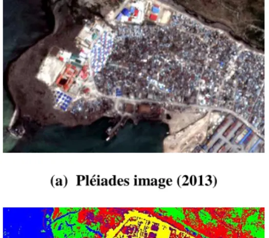
In this section, we discuss the results of the experimental validation of the developed hierarchical classifier on two datasets (see figure 7):

 A three-date series of panchromatic and multispectral Pléiades images acquired over Port-au-Prince (Haiti) in 2011, 2012, and 2013.

 Two pan-sharpened GeoEye acquisitions acquired over Port-au-Prince (Haiti) in 2009 and 2010. Five land cover classes have been considered for both data sets: urban (red), water (blue), vegetation (green), bare soil (yellow), and containers (purple). We note that these classes represent semantically high level land covers. However, a classification map associated with more detailed classes can be produced when a sophisticated ground truth is available. In the present work, manually annotated non-overlapping training and test sets were selected in homogeneous areas. Spatially disjoint training and test areas were used in all experiments to minimize correlation between training and test samples and prevent possible optimistic biases in accuracy assessment.

20 In the case of the Pléiades images, the finest resolution of the multiresolution pyramid (level 0) was set equal to the finest resolution of the input panchromatic images (i.e., 0.5 m). Co-registered multispectral images (at 2 m) were integrated in level 2 of the pyramid. To fill level 1, a wavelet decomposition of the panchromatic image was used. As a preliminary experiment, the combination of the proposed method with numerous wavelet operators, including Daubechies, biorthogonal, and reverse biorthogonal wavelets, symlets, and coiflets of various orders [33], was examined. The results were similar, and the main difference relied on the level of smoothness of the final classification map. On one hand, as shown in Figure 6, the average of the overall accuracies obtained on the test sets of all individual dates was remarkably stable as a function of the selection of the wavelet operator, suggesting that this selection is not critical in the application of the proposed approach. On the other hand, an exception was represented by the Daubechies wavelets of order 10 (db10) whose combination with the proposed multiresolution method resulted in higher accuracies than the other considered wavelet transforms. This wavelet operator will be used in all other experiments discussed in this paper (see Figure 6).

Figure 6: Pléiades data set: average of the overall accuracies obtained on the test sets of all individual dates results using several wavelet families.

The GeoEye image resolution is at 0.5 meters (the finest resolution of the multiresolution pyramid). Comments similar to those reported for the experiments with Pléiades images regarding the selection of the wavelet operator hold here as well, and db10 was used to fill level 1 and level 2 of the pyramid.

As discussed in Section II.A, the proposed method depends on four parameters, i.e., 𝛽 in (10) and (15), 𝜃 in (12) and (20), 𝜑 in (20), and 𝑅. the classification results included in the paper were obtained using the following parameter values: 𝛽 = 0.8, 𝜃 = 0.85, 𝜑 = 0.48, and 𝑅 = 2, i.e., three levels in each quad-tree. Including more decomposition levels generally assists in discriminating homogeneous land

83 84 85 86 87 88 89 90 b io r11 b io r68 co if1 co if3 _db1 d b 10 _db2 _db3 _db5 Dme y H aar rb io 11 rb io 22 rb io 33 rb io 44

sym10 sym2 sym25 sym5

Ov era ll a ccura cy (% ) Wavelet families

21 covers but might result in the removal of small-size image details [1, 15, 51, 52]. Indeed, with 𝑅 = 2, the classification map is generated at 50-cm spatial resolution for both data sets, while the coarsest scale corresponds to 2-m resolution. Including coarser-resolution features would generally favor spatial smoothness but may progressively hinder the capability to discriminate classes characterized by spatial details such as “buildings” and “containers.”

The value of 𝛽 was automatically optimized by applying the well-known pseudo-likelihood method to the training samples [27]. Accordingly, a user/operator does not have to perform a trial-and-error procedure to set 𝛽. In general, a lower value of 𝛽 prevents spatial oversmoothing at the price of an accuracy decrease on test samples located inside homogeneous regions associated with the same thematic class.

As 𝛽 is automatically optimized, the only free parameters are 𝜃 and 𝜑. According to (20), 𝜃 is the probability that a site, its parent on the same date and its parent on the previous date all share the same class label; 𝜑 is the probability that a site shares the same label of one of the two parents while the parents disagree. For (20) to define a probability distribution, 𝜃 and 𝜑 can take values in [0, 1] and [0, 0.5], respectively, in the case of 𝑀 = 5 classes. Figures 11 and 12 show the behavior of the overall accuracy of the proposed method on the test set as each one of these two parameters range in these intervals while the other parameter is fixed to the aforementioned reference values (i.e., 𝜃 = 0.85 and 𝜑 = 0.48). On one hand, these plots suggest that the method is sensitive to the values of 𝜃 and 𝜑. This is an expected result because they involve the causality of the model. On the other hand, limited sensitivity was observed and the overall accuracy remained higher than approximately 85% as long as 𝜑 and 𝜃 were larger than 0.4 and 0.85, respectively. On the contrary, it was basically for relatively extreme and not meaningful values of 𝜃 or 𝜑 that poor values of the overall accuracy were obtained. For example, 𝜑 = 0.2 implies that there is a 15% probability that the labels of a site and of its two parents are all different (see (20) with 𝑀 = 5). Because of the very high interscale and temporal correlations associated with the multiresolution data sets, this event is highly unlikely, and 𝜑 = 0.2 yields to significantly overestimating its chances of occurring in the classification process, thus affecting the overall accuracy. Similarly, 𝜃 = 0.5 implies a 12.5% probability that the parents of a site on the two dates agree on a certain class membership but the site disagrees, another outcome that is very unlikely because of interscale correlation and whose probability is overestimated.

Therefore, although the proposed method is overall sensitive to 𝜃 and 𝜑, the experimental analysis suggests that the meaning of the two parameters in relation to interscale and temporal correlation allows

22 a user/operator to rather easily determine values of or ranges on these parameters that lead to accurate classification maps.

Preliminary experiments also pointed out that the use of the MMD optimization technique resulted in a significant reduction in the number of iterations needed to estimate the class label of each pixel as compared to the direct maximization of the posterior marginals. To reach convergence in the case of one single level of a quad-tree including 1600 x1000 pixels and 5 classes, MMD required fewer than 1000 iterations. We recall that, in each MMD iteration, one individual pixel is examined. On the contrary, the direct choice of the class label that maximizes the posterior marginal on each pixel required to iterate over all 1600 x1000 pixels and 5 classes, thus taking a much longer time.

The results obtained by the proposed method were compared to those generated by: the technique in [1], used as a multiresolution single-date benchmark in both its (i) MPM- and (ii) MAP-based formulations; (iii) the MRF-based algorithm in [2], used as single-resolution multitemporal benchmark; (iv) a contextual combination of the K nearest neighbor and MRF-based approaches, used as a single-resolution single-date benchmark; and (v) the well-known K-means clustering technique, used as a basic unsupervised benchmark. The results of the proposed and previous techniques are reported in the following subsection along with further details on their applications.

2) Experimental Results and comparisons

In this section, we present the classification maps and discuss the corresponding classification accuracies that were obtained on the test set. Figure 9 and Table 1 refer to the results obtained using Pléiades images, and Figure 10 and Table 2 regard those obtained from the GeoEye acquisitions All computation times reported in the tables refer to a C++ implementation on an Intel i7 quad-core (2.40 GHz) 8-GB-RAM 64-bit Linux system.

The analysis of the classification maps has suggested that the proposed hierarchical method leads to accurate results.

In particular, several experimental comparisons were performed with methods exploiting multi- or single-resolution, multi- or single-date, supervised or unsupervised approaches. First, the results of the proposed technique were compared to the separate hierarchical classifications results obtained at individual dates using the multiresolution single-time method in [1], in both its MPM (Figure 9(c) and Figure 10(c)) and MAP formulations and using a 3 level pyramid with the following parameters: 𝛽 = 0.8

23 and 𝜃 = 0.85 (see Figure 9(d) and Figure 10(d)). We recall that several extensions of the method in [1] have been developed including the approach presented by Voisin et al. in [15] for the specific case of multisensor classification and based on the integration of the hierarchical MRF model of Laferté et al. in [1] with copula functions for merging data from both optical and SAR sensors within the same pyramid. In the present paper, the focus is on multitemporal classification with optical images and not on multisensor fusion. Accordingly, we used the original method in [1] for comparison purposes. The results of the comparison suggest the effectiveness of the proposed multitemporal hierarchical model in fusing the temporal, spatial, and multiresolution information associated with the input data (see Table 1). In practice, the use of one quad-tree structure with the MPM criterion yields “blocky” segmentation (see Figure 8 (a)). This phenomenon can be explained by the fact that two neighboring sites at a given scale may not have the same parent. In this case, a boundary appears more easily than when they are linked by a parent node. These blocky artifacts are avoided by the use of the multitemporal hierarchical structure proposed in this work in which causal relationships between parents and offspring in the same quad-tree are relaxed by the introduction of other causal relationships over time and scale (see Figure 8(b)). One of the main sources of misclassification in the single-date results is the confusion between the “urban” and “vegetation” classes; this misclassification is reduced in the multitemporal classification obtained by the proposed method because of the modeling of the temporal relationships among the input multiresolution data. Furthermore, as expected, the MAP criterion was poorly effective when applied to the considered hierarchical structure because errors were propagated from the root to the leaves and led to severe misclassifications, especially regarding the classes that most strongly overlap in the feature space (e.g., “urban” and “containers”; see Figures 9 and 10 (d)).

Second, in the context of multitemporal classification, the proposed classifier was compared to the multitemporal single-resolution MRF-based method proposed in [2]. It uses the mutual approach and consists in performing a bidirectional exchange of the temporal information between the (non-hierarchical) single-time MRF models associated with consecutive images in the sequence. In the form of an appropriate energy function, each single-time MRF model integrates three types of information (spectral, spatial contextual, and temporal contextual) using a multilayer perceptron (MLP) neural network to extract the spectral information. The results reported in Table 2 show that a better exploitation of the spatio-temporal information allowed the proposed cascade multiresolution approach to provide more accurate results than the previous mutual single-resolution approach in [2]. More generally, the mutual approach reduces the risk of propagating the classification error between consecutive dates, while the use

24 of the hierarchical schema provided more accurate classification maps, at least, on the considered data sets. Furthermore, because of the hierarchical aspects and the non-iterative algorithm, only few minutes were necessary to obtain satisfactory results using the proposed approach compared to those obtained by the mutual approach that required a much longer computation time (several hours). According to the formulation of the method in [2], this time included the times required to compute the texture features from the given image time series, to train and apply an MLP neural network for the image of each date using the backpropagation algorithm, and to estimate the parameters of the corresponding MRF model using the case-specific parameter optimization procedure in [3].

The classification maps obtained using the well-known K-nearest-neighbors (K-NN) method are also shown in Figures 9 and 10 (h). K-NN was used as a benchmark parametric classifier. It is non-contextual, so to perform a fair comparison between the proposed method and a spatial-contextual technique, it was combined with an MRF model. A hidden MRF whose unary term was expressed in terms of the pixelwise posterior probabilities estimated by K-NN and whose contextual term was represented by an isotropic Potts model was used. K = 30 was estimated by cross validation on the training set, and the smoothing parameter of the Potts model was optimized using the automatic method in [36], which is based on the Ho-Kashyap algorithm. The numerical results on the test sets suggest that this single-scale MRF-based method (see Tables 1 and 2) leads to rather poor accuracy and severe spatial oversmoothing as shown in Figures 9 and 10(g). This is consistent with the fact that this combined K-NN + MRF classifier is intrinsically single-resolution and single-date, and can exploit neither the multiresolution nor the multitemporal structure of the input data set. In the map in Figure 10(g), obtained from GeoEye data, the combined K-NN + MRF well discriminated the “water” and “urban” classes but almost did not identify the other thematic classes due to the strong spectral overlapping and the imbalance between the training sample sizes of these classes.

Finally, a further comparison was performed between the results of the proposed method and those of an unsupervised algorithm. K-means was used for this benchmark comparison as a well-known consolidated approach, and was applied with K = 5. This number of clusters was used to match the number of classes in each data set. The clusters obtained by K-means generally do not coincide with the thematic classes of a supervised classification problem. An alternate strategy could be to, first, apply K-means using a significantly larger number of clusters, and then, perform a cluster-to-class assignment either manually or on the basis of the training set. In either case, this assignment would incorporate prior knowledge. This experiment was meant as a benchmark comparison with an unsupervised method using no prior

25 knowledge. Accordingly, the simple choice K = 5 was accepted. As expected due to its unsupervised, non-contextual, and single-resolution formulation, K-means performed the worst in terms of classification accuracy, while it exhibited the lowest computation time (see figures 9, 10 (h)).

Port au Prince

Pléiades ©CNES (2011), distribution Airbus DS

Port au Prince

Pléiades ©CNES (2012), distribution Airbus DS

Port au Prince

Pléiades ©CNES (2013), distribution Airbus DS

Port au Prince ©GeoEye (2009),

Port au Prince ©GeoEye (2010), Figure 7: Examples of time series images acquired over Port-au-Prince (Haiti)

(a) (b)

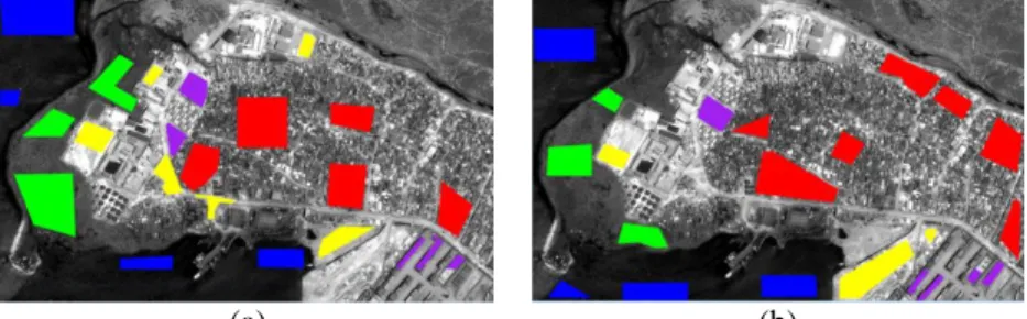
Figure 13: Ground truth for the Pléiades image acquired in 2013: (a) training set, (b) test set

Class name and color # of pixels in training set # of pixels in test set

Water(blue) 49 057 45 790

Urban (red) 75 508 72 327

Vegetation (green) 50 688 27 086 Bare soil (yellow) 29 333 25 541 Container (purple) 16 064 14 652

Table 3: Number of training and test samples on the panchromatic pixel lattice of the Pléiades image (1600 x1000 pixels) acquired in 2013

26

(a) Pléiades image (2013) (b) Ground Truth (training+test sets)

(c) Laferté et al. (with MPM criterion) [1] (d) Laferté et al. (with MAP criterion) [1]

(e) Melgani et al. [2] (f) The proposed method

(g) K-NN + MRF method (h) K-means

Figure 9: Classification maps obtained from Pléiades images, (© CNES distribution Airbus DS). Legend: urban (red), water (blue), vegetation (green), bare soil (yellow) and containers (purple).

27

(a) GeoEye image (2010) (b) Ground Truth (training+test sets)

(c) Laferté et al. (with MPM criterion) (d) Laferté et al. (with MAP criterion)

(e) Melgani et al. (f) The Proposed method

(g) KNN-MRF method (h) K-means

Figure 10: Classification maps obtained from GeoEye images. Legend: urban (red), water (blue), vegetation (green), bare soil (yellow) and containers (purple).

28

(a) (b)

Figure 8: (a) Detail of two maps in Figure 7: blocky artefacts obtained using the method in [1] in its MPM formulation (b) reduction of these blocky artefacts using the proposed method.

Port-au-Prince, Haiti

urban water vegetation bare soil containers overall accuracy

computation time Proposed method 81.62 % 100 % 90.69 % 92.82 % 62.82 % 85,59 % 480 seconds Laferté et al. method

using MPM criterion

77.45 % 88.62 % 72.59 % 86.02 % 57.02 % 76.34 % 160 seconds Laferté et al. Method

using MAP criterion

56.14 % 100% 81,90 % 87.02% 73.21% 79.65 % 220 seconds Melgani et al. method 80.63 % 100 % 86.33 % 87.61 % 69.61 % 84,83 % ≈1 hour

K-NN + MRF 96,84% 92,42% 47.15 % 71.83 % 16.75 % 64.99% 90 seconds K-means 12.37% 98.63% 59.18% 91.66 % 29.42 % 58.25 % 20s

Table 1. Classification accuracies on the test set of the Pléiades dataset: class accuracies (producer’s accuracies), overall accuracy, and computation time.

Experiments were conducted using one (1600x1000) image in level 0, one (800x500) image in level 1 and four (400x250) bands in level 2 on an Intel i7 quad-core (2.40 GHz) 8-GB-RAM 64-bit Linux system.

Port-au-Prince, Haiti

urban water vegetation bare soil containers overall accuracy

computation time Proposed method 87.59 % 100 % 98.12 % 72.82 % 82.27 % 88,16 % 345 seconds Laferté et al. method

using MPM criterion

77.45 % 100 % 88.34 % 66.22 % 67.87 % 79.97 % 90 seconds Laferté et al. method

using MAP criterion

64.52 % 100% 92.15 % 85.62% 49.47 % 78.35 % 140 seconds Melgani et al. method 80.63 % 100 % 89.79 % 70.54 % 74.29 % 83,05 % ≈1 hour

K-NN + MRF 100% 100% 0% 0% 12.28% 42.45 % 40 seconds K-means 88.97% 100% 88.14% 45.6 % 36.96 % 71.93 % 15 seconds

Table 2. Classification accuracies on the test set of the GeoEye dataset: class accuracies (producer’s accuracies), overall accuracy, and computation time.

Experiments were conducted using one (1600x800) image in level 0, one (800x400) image in level 1 and one (400x200) bands in level 2 on an Intel i7 quad-core (2.40 GHz) 8-GB-RAM 64-bit Linux system.

29

(a) (b)

Figure 11. Overall accuracy of the proposed method on the test set of the Pléiades data set as a function of the parameters (a) 𝜑 and (b) 𝜃.

Detail on the Pléiades image 𝜃 = 0.7, 𝜑 = 0.45

𝜃 = 0.85, 𝜑 = 0.2 𝜃 = 0.85, 𝜑 = 0.45

Figure 12. Details of the the classification maps obtained by the proposed method when applied to the Pléiades data set with different values of 𝜃 and 𝜑.

65 70 75 80 85 90 0,2 0,3 0,4 0,49 O ve ral l Ac cu rac y (%) Values of 𝜑 81 82 83 84 85 86 0,5 0,7 0,85 0,9 O ve ral l A cc ur ac y (%) Values of 𝜃

30

IV. CONCLUSION

In the proposed method, multidate and multi-resolution fusion is based on explicit statistical modeling. The method combines a joint statistical model of the considered input optical images through hierarchical Markov random field modeling, leading to a statistical supervised classification approach. We have developed a novel MPM-based hierarchical Markov random field model that considers multitemporal information and, thus, supports the joint supervised classification of multiple images taken over the same area at different times and different spatial resolutions. We analyzed the results obtained with the proposed method through experiments with multitemporal Pléiades and GeoEye data sets. The experimental results suggest that the method is able to provide accurate classification maps. The proposed algorithm was compared to a previous single-date multiresolution method and a previous multidate single-resolution method, both based on MRF models associated with suitable (hierarchical or single-scale) pixel lattices and a couple of well-known classifiers including a contextual combination of the K nearest neighbor and MRF-based approaches, used as a single-resolution single-date benchmark; and the K-means clustering technique, used as a basic unsupervised benchmark. The proposed technique was demonstrated to be advantageous in terms of the classification accuracy on the test set, the spatial regularity of the classification maps, the minimization of spatial artifacts, and the tradeoff with respect to computation time. These results suggest the effectiveness of the algorithm in fusing both multitemporal and multiresolution information for supervised classification purposes and confirm that MRF models represent a powerful fusion tool in remote sensing.

The computational advantages of hierarchical MRFs, for which exact recursive formulations of the MPM decision rule are feasible with no need for time-expensive Metropolis or Gibbs sampling procedures, has also been confirmed by the experimental results of the proposed method and those of the benchmark single-resolution multiresolution classifier.

The proposed method is based on an MRF model on a case-specific topology that comprises multiple hierarchical quad-trees, each associated with an acquisition date. Wavelet transforms are used to fill in those levels of each quad-tree that are associated with input remote sensing imagery. The selection of the wavelet operator among a large family of possible transforms was not critical because most transforms lead to classification results with similar accuracies. Nevertheless, Daubechies wavelets of order 10 yielded higher accuracies than the other considered transforms. As a future extension of this method, the automation of the selection of the wavelet operator using, for example, a dictionary of multiple transforms [35] could be incorporated in the developed model and classifier. Similarly, the pseudo-likelihood method