Designing mechanisms with shape memory alloys and permanent magnets

Designing Mechanisms with Shape Memory Alloys

and Permanent Magnets

by

B.S., The

Nicholas E. Kottenstette Mechanical Engineering (1995) Catholic University of America

Submitted to the Department of Mechanical Engineering in Partial Fulfillment of the Requirements for the Degree of

Master of Science at the

Massachusetts Institute of Technology February 1997

@ 1997 Massachusetts Institute of Technology. All rights reserved.

Signature of Author...

Certified by ... C

Accepted

Department of Mechanical Engineering

___,____v _{4, 1997}

Woodie C. Flowers Pappalardo Professor of Mechanical Engineering -,,<7-ft,.hesis Supervisor by

...

_

...

Ain A. Sonin Chairman, Department Committee on Graduate Students

APR 1 6

1997

Alf -il

Designing Mechanisms with Shape Memory Alloys

and Permanent Magnets

by

Nicholas E. Kottenstette

Submitted to the Department of Mechanical Engineering on February 3, 1997, in Partial Fulfillment of the

Requirements for the Degree of Master of Science

ABSTRACT

A computer program has been created which assists an engineer to develop mechanisms which use Shape Memory Alloys (SMAs) and permanent magnets. The computer program simulates the following systems:

1. An electrically-heated Ni49TiS wire actuating a constant force bias spring. 2. An electrically-heated Ni49Ti51 wire actuating a linear bias spring.

3. A bi-stable mechanism employing Ni₄₉Ti51 wires and permanent magnets.

The simulations aid the engineer in creating reliable Shape Memory Alloy actuators for specific life-cycle and environmental temperature requirements.

Temperature-strain curves of three SMAs supplied by Dynalloy (Ni49Ti,,51, Ni49Ti44Hf7 and

Ni49Ti44Cu7) were experimentally obtained. The simulated temperature-strain curve for the

Ni49Ti51 wire approximately matched the experimental results, which led to the

manufacturing predictions for Dynalloy's Ni49Ti51 SMAs. The Ni49Ti4Hf, wires shrank

only 1.5% (4% shrink was expected) and their Martensite Finish temperature was no greater than that of the Ni49Ti,, wires.

Life-cycle tests were performed on Ni49TiS wire at an actuating stress of 160 MPa. Two

Ni49Ti51 wires cycled approximately 1,000,000 times under a 160 MPa stress; however, using the same apparatus, two other Ni49Ti51 wires cycled approximately 10,000 times under the same 160 MPa stress.

Experimental force-gap curves were obtained for Ceramic, Samarium Cobalt, Neodymium Iron Boron, and Bonded Neodymium Iron Boron magnets. These experimental curves were used to create 2 correction factors for future force-gap curve simulations.

Thesis Supervisor: Woodie C. Flowers

Acknowledgments

My wife,

Maryellen Kottenstette Professor Woodie Flowers DEKA Research and Development Gustavo Buhacoff

Dr. Kingston Owens

Professor Frank McClintock Professor David Trumper

Professor Anuradha Annaswamy Raymond Hardin

Michael Bush My parents,

Designing Mechanisms with Shape Memory Alloys

and Permanent Magnets

List of Figures ... 7

List of Tables ... 12

1 Shape Memory Alloys and permanent magnets ... 13

1.1 An introduction to Shape Memory Alloys ... 14

1.2 An introduction to permanent magnets ... 18

2 Modeling SMA-actuated systems ... 23

2.1 Modeling an electrically-heated Ni₄₉Ti51 wire actuating a constant force bias spring ... 24

2.2 Modeling an electrically-heated Ni49Ti51 wire actuating a linear bias spring ... 26

2.3 Modeling a bi-stable mechanism employing Ni49Ti51 wires and permanent magnets ... 28

3 Computer simulations of SMA-actuated systems ... 34

3.1 Simulation of an electrically-heated Ni49Ti51 wire actuating a constant force bias spring ... 34

3.2 Simulation of an electrically-heated Ni49TiS wire actuating a linear bias spring ... 39

3.3 Simulation of a bi-stable mechanism employing Ni₄₉Ti51 wires and permanent magnets ... 44

4 Conclusions and Recommendations ... 51

Appendix A: Users Manual for Design Program ... 53

Appendix B: Modeling Shape Memory Alloys ... ... 78

Appendix D: Appendix E:

Model for Permanent Magnets ... 129 Permanent Magnet Experiments and Results ... 151 B ibliography ... 161

Figure

Figure 1. Stress-strain curve for SMAs consisting of Nickel and Titanium ... 15

Figure 2. Arrangement required to create a SMA which can contract and elongate without being plastically deformed ... 16

Figure 3. Half of a Samarium Cobalt magnet and a low-carbon steel torus ... 19

Figure 4. B-H curves for Samarium Cobalt and low-carbon steel ... 20

Figure 5. An electrically-heated Ni49Ti51 wire actuating a constant force bias spring... 24

Figure 6. An electrically-heated Ni49Ti51 wire actuating a linear bias spring.. 26

Figure 7. A bi-stable mechanism employing Ni49Ti51 wires and permanent m agnets ... 28

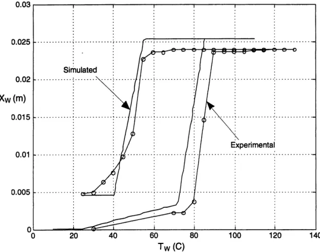
Figure 8. Simulated and experimental temperature-position curves for a 4.3 MPa biased Flexinol 90-110 wire ... 35

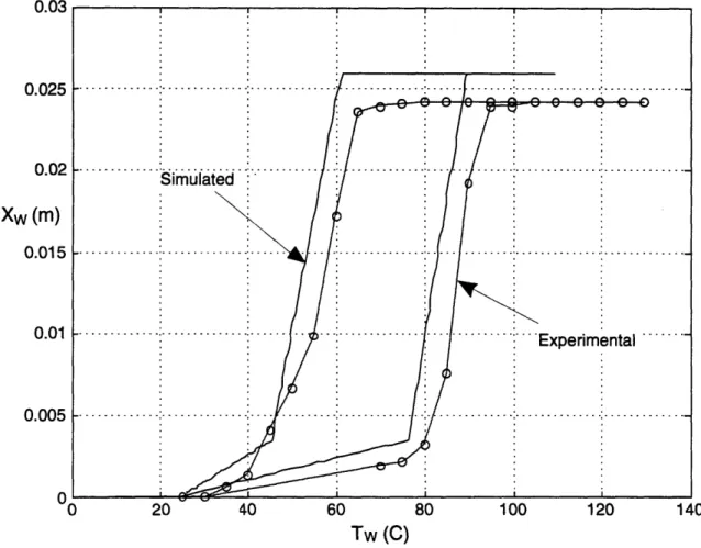
Figure 9. Simulated and experimental temperature-position curves for a 47.3 MPa biased Flexinol 90-110 wire ... 36

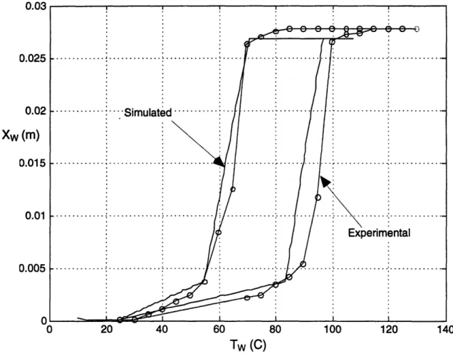
Figure 10. Simulated and experimental temperature-position curves for a 86.0 MPa biased Flexinol 90-110 wire ... 37

Figure 11. Simulated and experimental temperature-position curves for a 150.4 MPa biased Flexinol 90-110 wire ... 38

Figure 12. Simulated temperature-time curve for Ni49Ti,1 wire ... 40

Figure 13. Simulated length-time curve for Ni49Ti51 wire ... 41

Figure 14. Simulated stress-time curve for Ni₄₉Ti 5 wire ... 42

Figure 15. Simulated temperature-strain curve for Ni49Ti51 wire ... 43

Figure 16. Simulated magnetic force-gap curve for Samarium Cobalt ... 44

Figure 17. Resulting magnetic torque-angular position curve from Samarium Cobalt pendulum ... 45

Figure 18. Simulated angular position-time curve for steel lever ... .47

Figure 19. Simulated stress-time curve for Ni49Ti51 wire (wire 2) ... 48

Figure 20. Simulated temperature-strain curve for Ni49Ti' wire (wire 1) ... 49

Figure Al. An electrically-heated Ni49Ti,5 wire actuating a constant force bias spring ... ... 54

Figure A2. Design menu used to simulate an electrically-heated Ni49Ti51 wire .. 55

Figure A3. The "Flexinol 90-110 Wires" screen ... 57

Figure A4. The "Mondo-tronics Ribbon Wires" screen ... 58 Page

Figure Figure Figure Figure Figure Figure Figure Figure A5. A6. A7. A8. A9. A10. All. Figure A12. Figure Figure Figure Figure Figure Figure Figure Figure Figure Figure A13. A14. A15. A16. A17. A18. A19. A20. A21. A22. Figure B 1. Figure B2. Figure B3. Figure B4. Figure B5. Figure B6. Figure B7. Figure B8.

The "Create Your Own Wires" screen ... 59

The "Create Force History" screen (constant force bias option) ... 60

Simulated temperature-strain curve for Ni49Ti51 wire ... 61

An electrically-heated Ni49Ti51 wire actuating a linear bias spring .. 62

The "Create Force History" screen (linear spring bias option) ... 63

Simulated stress-time curve for Ni49Ti51 wire ... 64

A bi-stable mechanism employing Ni49Ti51 wires and permanent magnets ... 65

Main menu used to simulate a bi-stable mechanism employing Ni49Ti51 wires and permanent magnets ... 66

The "SMA Wires" screen ... 67

The "Bias Springs" screen ... 68

The "Assembly Dimensions" screen ... 69

The "Magnet and Friction Torque" screen ... 70

Magnetic torque-angular position and normal force-angular position curves ... 71

The "Heating The Wires" screen ... 72

Electrical square wave to heat Ni49Ti51 wires ... 73

The "Lever Inertia" screen ... 74

The "Plot Results" screen ... 75

Simulated angular position-time curve for steel lever ... 77

Generalized model for a Shape Memory Alloy ... 78

Thermal conductivity-temperature curve for air ... 80

Prandtl-temperature curve for air ... 81

Curve relating logl0(gp/v2) to temperature for air ... 82

Temperature-strain curve model for a SMA ... 84

Experimental temperature-strain curve of a 4.3 MPa biased Ni49Ti51 wire ... 86

Experimental temperature-strain curve of a 47.3 MPa biased Ni49Ti51 wire ... 87

Experimental temperature-strain curve of a 86.0 MPa biased Ni49Ti51 wire ... 88

Figure Figure B9. Figure B 10. Figure B 11. Figure B 12. Figure B13. Figure B 14. Figure B 15. Figure B16. Figure Figure Figure B17. B18. B19. Figure B20. Figure B21. Figure C 1. Figure C2. Figure C3. Figure C4.

Experimental temperature-strain curve of a 150.4 MPa biased

N i49Ti51 w ire ... 89

Experimental temperature-strain curve of a 4.3 MPa biased

Ni49Ti44Cu7 wire ... 90

Experimental temperature-strain curve of a 43.0 MPa biased

Ni₄₉Ti₄₄Cu7 wire ... ... 91

Experimental temperature-strain curve of a 86.0 MPa biased

Ni49Ti44Cu7 wire ... 92

Experimental temperature-strain curve of a 150.4 MPa biased

Ni49Ti44Cu7 wire ... . 93

Transformation temperatures-stress curves (Ms, Mf, As, Af)

for Ni49Ti51 wire ... 94

Austenite finish temperature-cycle curves for Ni49Ti51 wires with

different heat-treatments ... 95 Martensite start temperature-cycle curves for Ni49Ti51 wires with different heat-treatments ... 96 Unrecovered strain-stress curve for Ni49Ti5 wire ... 98 Shrink loss-cycle curve for Ni4 9Ti51 wire ... 99 Creep-cycle curves of Ni49Ti1 wires

(4000_{C, 425}0_{C and 600}0_{C heat-treatments) under 69.0 Mpa ... 101}

Creep-cycle curves of Ni49Ti51 wires

(4000_{C, 425}0_{C and 600}0_{C heat-treatments) under 207.0 MPa .... 102}

Contraction-cycle curve for pre-creeped Ni49Ti51 wire under

69.0 MPa ... 103 Experimental apparatus used to obtain temperature-strain curves ... 106 Experimental temperature-strain curve of a 4.3 MPa biased

N i49Ti,, w ire ... 110 Experimental temperature-strain curve of a 47.3 MPa biased

Ni49Ti51 wire ... ... 111

Experimental temperature-strain curve of a 86.0 MPa biased

N i49T i51 w ire ... 112

Figure Figure C5. Figure C6. Figure C7. Figure C8. Figure C9. Figure C10. Figure C11. Figure C12. Figure C13. Figure C14. Figure Figure C15. C16. Figure D 1. Figure D2. Figure D3. Figure D4. Figure D5. Figure D6. Figure D7. Figure D8. Figure D9. Figure D10.

Experimental temperature-strain curve of a 150.4 MPa biased N i49Ti51 w ire ...

Transformation temperatures-stress curves (Ms, Mf, As, Af) for Ni49Ti51 wire ...

Experimental temperature-strain curve of a 4.3 MPa biased N i4 9Ti4 4Cu7 wire ...

Experimental temperature-strain curve of a 43.0 MPa biased N i49Ti44Cu, wire ...

Experimental temperature-strain curve of a 86.0 MPa biased N i49Ti44Cu7 wire ...

Experimental temperature-strain curve of a 150.4 MPa biased N i49Ti44Cu7wire ... 113 114 116 117 118 119 Transformation temperatures-stress curves (Ms, Mf, As, Af)

for Ni49Ti4 4Cu7 wire ... 120

Experimental temperature-strain curve of a 4.3 MPa biased N i49Ti44H f7 wire ... 122

Experimental temperature-strain curve of a 150.4 MPa biased N i49Ti44H f7 wire ... 123

Experimental apparatus used for life-cycle testing of a Ni49Ti51 wire ... 124

Digital electronic circuit used to thermally cycle Ni49Ti51 wire ... 125

Adjustable voltage supply used to electrically heat Ni49Ti51wire ... 125

Magnetic fields of a permanent magnet located in free-space and on a steel block ... Demagnetization curves for permanent magnets ... Force-gap curves for Samarium Cobalt ... Force-gap curves for Neodymium Iron Boron ... Force-gap curves for Ceramic 5 ... Force-gap curves for Ceramic 8 ... Force-gap curves for Bonded Neodymium Iron Boron Experimental relationship between Cf, and DM/Lm ... Experimental relationship between Cf2 and DM/Lm ... Corrected force-gap curves for Samarium Cobalt .... 130 ... 133 ... 138 ... 139 ... 140 ... 141 ... 142 ... 144 ... 145 ... 146 Page

Figure Figure D 11. Figure D12. Figure D13. Figure D14 Figure El. Figure E2. Figure E3. Figure E4. Figure E5. Figure E6.

Corrected force-gap curves for Neodymium Iron Boron ... Corrected force-gap curves for Ceramic 5 ...

Corrected force-gap curves for Ceramic 8 ...

Corrected force-gap curves for Bonded Neodymium Iron Boron .. 147 148 149 150

Experimental apparatus used for testing permanent magnets ... 152

Experimental force-gap curve for Samarium Cobalt ... 156

Experimental force-gap curve for Neodymium Iron Boron ... 157

Experimental force-gap curve for Ceramic 5 ... 158

Experimental force-gap curve for Ceramic 8 ... 159

Experimental force-gap curve for Bonded Neodymium Iron Boron ... 160

Table

Table C1. Experimental temperature-contraction results for Ni49Ti51 wire .... 109

Table C2. Experimental temperature-contraction results for Ni49Ti44Cu7 wire. . 115 Table C3. Experimental temperature-contraction results for Ni49Ti44Hf7 wire.. 121

Table D1. Residual flux densities and coercivities of permanent magnets .... 134 Table El. Experimental force-gap results for permanent magnets ... 155

1

Shape Memory Alloys and permanent magnets

Shape Memory Alloys (SMAs) and permanent magnets are non-linear materials which can be described by hysteresis loops. Together, they can be used to form bi-stable

mechanisms. SMAs can be electrically heated in order to move a permanent magnet between two stable states. Figure 7 illustrates a bi-stable mechanism in which two SMA

wires are used to toggle a steel lever which is biased by a permanent magnet pendulum. The bi-stable mechanism utilizes the magnet's constant holding force capabilities, and the

SMAs' actuating capabilities. The mechanism is energy efficient, because it eliminates the need for the SMA to be continuously heated in order to maintain a specific position. In order to simulate the bi-stable mechanism, methods to simulate SMAs and permanent magnets will be developed.

Shape Memory Alloys are alloys which, when properly manufactured, can contract and elongate approximately 4% of their initial length. This ability to contract and elongate

allows SMAs to be used as actuators. In order for reliable SMA actuators to be developed, the engineer needs to be aware of the limitations associated with SMAs. For example, a properly designed SMA actuator will operate with environmental temperatures no greater than 500C. These and other limitations of SMAs are discussed as this document shows how to simulate the following systems:

1. An electrically-heated Ni49Ti51 wire actuating a constant force bias spring.

2. An electrically-heated Ni49Ti51 wire actuating a linear bias spring.

3. A bi-stable mechanism employing Ni49Ti,5 wires and permanent magnets.

Ni49Ti5l wires are a primary SMA used in industry. The system simulations shown above

are performed using the software package MATLAB®. These simulations illustrate how to manufacture Ni49Ti5 1 wire, perform life cycle analysis, and tolerance studies on the

systems. Section 1.1 provides a more detailed discussion of SMAs.

Permanent magnets are in many of the products people use. Permanent magnets can be found in speakers, electric motors for VCRs and blenders, on credit cards and on

refrigerators holding up memos. This document discusses how to determine the resulting permanent magnetic holding force on a refrigerator with a low-carbon steel shell. It shows

how the holding force changes when various non-magnetic items with different thicknesses are placed between the permanent magnet and the refrigerator. It will show that, for the appropriate holding force to be obtained, the steel shell requires a minimum thickness in order to avoid magnetic saturation. Section 1.2 provide a more detailed discussion of this problem.

1.1 An introduction to Shape Memory Alloys

In the 1960s Buehler and Wiley invented the Shape Memory Alloy NiTiNOL (Nickel Titanium Naval Ordinance Laboratories); however, significant research involving SMAs did not occur until the early 90s. Baz (1990), Liang and Rogers (1990) began to

investigate the dynamic behavior and modeling of SMAs. Thoma (1992) wrote a paper on manufacturing stable SMA wires consisting of Ni49Ti51. Baz developed an empirical dimensionless model to determine the resulting thermal time constants, and maximum displacement of a spring and mass biased actuator. Liang and Rogers developed a constitutive model for the phase transformation dynamics and stress-strain-temperature relations for SMAs. Thoma discussed the SMAs' changing properties due to cycling under an applied stress. Appendix B incorporates the work of Thoma, Liang and Rogers, along with recent experimental results (Appendix C), in order to develop a more complete dynamic model for Ni49Ti5,, wires.

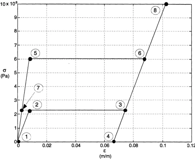
A Shape Memory Alloy is an alloy which can be transformed between two phases by changing its temperature. The phase transformation occurs at temperatures which are below the recrystalization temperature. The two phases are known as the Martensite phase and Austenite phase. Figure 1 shows the resulting stress-strain history for a SMA

10ox

(Pa)

12 (m/m)

Figure 1. Stress-strain curve for SMAs consisting of Nickel and Titanium. When the SMA is in its Martensite phase, it can be strained from point 1 to point 2, at which point the wire yields at 224 MPa with a strain of .008 m/m (note the SMAs'

Young's modulus is 28 GPa). The SMA is further strained to point 3 (.0746 m/m) under a near constant stress (224 MPa). The SMA is then released as it recovers to point 4 with a final unrecoverable strain of .066 m/m. When the SMA is heated to its Austenite phase, the deformed SMA will recover the plastic strain from point 4 to point 1. When the SMA is in its Austenite phase it is in a super-elastic state. The SMA can be stretched from point 1 to point 5 at which point the wire yields at 600 MPa with a strain of .008 m/m (note the SMAs Young's modulus is 75 GPa). The SMA continues to be strained under a constant 600 MPa stress until the strain is .088 m/m at point 6. The stress in the SMA is reduced in order for the wire to return to point 3 (note the SMAs' Young's modulus is now at 28 GPa because it is in a stress-induced Martensitic state). As the stress continues to be reduced, the SMA recovers its strain to point 7, and then to point 1 (in which the SMAs Young's modulus is now 75 GPa because it is no longer in a stress-induced Martensitic state). So

long as the SMA remains in its Austenite phase, it can be continually cycled from points 1 to 5 to 6 to 3 to 7 to 1. Point 8 represents the ultimate strength of the SMA before it breaks (1,000 MPa). This curve was approximated by information given by Gilbertson (1994), in which the maximum recovery stress (600 MPa), Martensite Young's modulus (28 GPa), Austenite Young's modulus (75 GPa) and the ultimate stress (1,000 MPa) are given. The Martensite yield stress was estimated by multiplying the yield strain of the Austenite by the Young's modulus of the Martensite. The behavior of the stress-strain curve is based on an article written by Wayman (1993). Figure 2 illustrates the arrangement required to create a Shape Memory Alloy which can contract and elongate without needing to be plastically deformed.

4Lwt

1.04Lwi 00

Figure 2. Arrangement required to create a SMA which can contract and elongate without being plastically deformed.

In its Martensite state, a SMA wire is elongated to a total length (L,,) which is

approximately 4% of its initial length (L,,). The deformed wire is then constrained at both ends. The constrained wire is then heated to its Austenite finish temperature. Since the wire is constrained, it is unable to recover and remains in a stress-induced Martensite state. The wire is then cooled to below its Martensite finish temperature at which point it

"remembers" its former stress-induced Martensite state. This heating and cooling of the constrained wire should be repeated approximately five more times. After the training is

complete, the SMA is now capable of shrinking to L, and elongating 4% to L,, with a 70 MPa bias stress.

ý

leo

This process generates in-built microstresses in the parent phase that in turn program the specimen to behave as in a stress-induced Martensitic

transformation. That is, the microstresses favor only a single orientation of Martensite on subsequent cooling, which produces a spontaneous

deformation.

- Wayman (1990) There are over 10,000 United States patents on SMAs and their

applications. Few of these patents have resulted in viable products.

-Zhang, Zee and Thoma (1996) Some successful products are superelastic eyeglass frames, pipe couplings, and

orthodontic arch wires. The eye glass frames can be bent around a finger and still return to their initial state. The pipe couplings, manufactured by Raychem, are shipped in liquid nitrogen in a deformed Martensitic state (point 4 of Figure 1). The coupling is then removed and placed around two pipes to be connected. As the coupling warms, it

transforms into Austenite and attempts to recover to point 1 of Figure 1. If the pipes are the correct size, the superelastic coupling will still remain strained under a 224 MPa stress. This principle has also been applied to electrical connectors. The superelastic orthodontic arch wires are able to provide a constant bias stress in the patient's mouth as it changes shape, thus reducing the need for adjustments.

No high life cycle (over 10,000 cycles) SMA actuator currently exists which has made any significant market impact.

Failure in the application of SMAs is primarily due to the lack of knowledge of many scientists and engineers on the limitations of SMAs and how to process SMAs to achieve long lived and stable SMA members.

-Zhang, Zee and Thoma (1996)

The simulation programs presented address these limitations and enable engineers to design high life cycle SMA actuators.

1.2 An introduction to permanent magnets

Permanent magnetism has been observed since the Greeks discussed the repelling and attractive properties of magnes, otherwise known as a lodestone (Fe304), which was discovered in Magnesia, an ancient city in Asia Minor. Some authors who have published texts specifically on permanent magnet design are Parker (1962), Moskowitz (1995), McCaig (1977) and Campbell (1994). Livingston (1996) provides numerous examples of permanent magnet applications. In his fifth edition of Electric Machinery, Fitzgerald

(1990) introduced two new sections which provide a method for relating permanent magnetic fields to resulting mechanical torque and forces. The method introduces a fictitious coil wrapped around a permanent magnet which can reduce the flux density to zero. This enables the magnetic field energy and corresponding forces to be determined. Fitzgerald's method is applied to determine the magnetic pulling force on a steel block. The theoretical results are compared to experimental results in Appendix D. Two correction

factors are determined in order to match the theoretical results to the experimental results. The flux density (B) and magnetizing force (H) are used to describe magnetic materials. The flux density is the ratio of the total flux (0) to the cross-sectional area through which it passes. The magnetizing force is the ratio of the mean magnetomotive force (mmf) to a

given length of a closed path. The product of the flux (Webers) and the magnetomotive force (Ampere-turns) results in energy (Joules); hence, the product of B (Weber/m2 or Tesla) with H (Ampere-turns/m) results in energy per unit volume (Joules/m3_{). Figure 3}

shows a torus in which one half is a Samarium Cobalt magnet and the other half is a low carbon steel torus. Figure 4 illustrates their corresponding B-H curves. Equations Dl and

D2 are used to relate the flux density and magnetizing force of the permanent magnet to the low carbon steel.

AM =

As

Figure 3. Half of a Samarium Cobalt magnet and a low-carbon steel torus. The length of the flux path in the magnet is equal to the length of the flux path in the steel; hence, equation D1 implies that the magnetizing force of the magnet is equal to the negative magnetizing force of the steel. The sectional area of the magnet is equal to the cross-sectional area of the steel; hence, equation D2 implies that the flux density of the magnet is equal to the flux density of the steel.

2 1 B (Wb/m2) o -1 -2 .--10 -8 -6 -4 -2 0 2 4 6 8 10 x 10 H (A-t/m)

Figure 4. B-H curves for Samarium Cobalt and low-carbon steel.

Using the results from equations D1 and D2 in conjunction with B-H curves of Figure 4, the resulting flux density and magnetizing force for the permanent magnet and low carbon steel are as follows:

* BM = B = 1.025 Tesla

* HM = -Hs = -17.0 kA/m

Note that the results indicate that the steel became saturated. When the steel is unsaturated it can possess a flux density up to 1.0 Tesla with a corresponding magnetizing force of 3.33 kA/m. The flux density in this example has increased only by 2.5%; however, the resulting magnetizing force has increased by 410%. In order to maximize the flux density in a permanent magnet the magnetizing force needs to be minimized. In order to minimize the magnetizing force, the flux of the magnet needs to be directed by a "soft magnetic

Samarinum

Cobalt

...

..

.

... i ... i ... ! ... ....

(.65% C)

-...

.

..

... i...i...

-... i...IC. ..

....

I..

He

:

:

:

: He :Hci

material" (for example, a low-carbon steel torus). The "soft magnetic material" can not become saturated by the flux. This can be accomplished by making the cross sectional area of the "soft magnetic material" approximately equal to the cross-sectional area of the permanent magnet.

Figure 4 indicates two additional variables which define the shape of the curves: the coercivity (He) and the intrinsic coercivity (Hci). A third variable, the remanent

magnetization (B,), is also used to define the shape of the curves. The coercivity is the magnetizing force in which the flux density is zero. The intrinsic coercivity is the magnetizing force required to reverse the polarization of the magnet. The remanent

magnetization is the flux density when the magnetizing force is zero. The arrows in Figure 4 indicate the path dependency of the magnetic hysteresis loop. For example, the polarity of the magnet in Figure 3 is reversed as follows:

1. The magnet has the following flux density and magnetizing force: SBM = 1.025 Tesla

* HM = -17.0 kA/m (second quadrant) 2. A coil is wrapped around the magnet:

* the coil has 10,000 turns

* LM = .01 meters

* 1 Amp flowed through the coil

* The resulting magnetizing force (HM) was -1,000 kA-turns/m

* This magnetizing force is greater than the intrinsic coercivity; hence, the magnetic polarity was reversed.

3. The current was then brought back to 0 Amps leaving the magnet with the following values:

* BM = -1.025 Tesla

* HM = 17.0 kA/m (fourth quadrant)

Figure 4 indicates that the intrinsic coercivity equals the coercivity for the steel bar. Alnico magnets have a similar problem; hence, they will not be tested. Ceramic 5, Ceramic 8, Neodymium Iron Boron and Bonded Neodymium Iron Boron magnets have hysteresis

loops similar to the Samarium Cobalt magnet (linear in the second quadrant); hence, these magnets will be tested and compared. The predicted theoretical results and correction factors for these permanent magnets are discussed in Appendix D. The experimental permanent magnet pulling force results are presented in Appendix E.

2

Modeling SMA-actuated systems

Section two develops the models for the following systems:

1. An electrically-heated Ni49Ti51 wire actuating a constant force bias spring.

2. An electrically-heated Ni49Ti~ wire actuating a linear bias spring.

3. A bi-stable mechanism employing Ni49Ti51 wires and permanent magnets.

The models for these systems can be applied if the actuating wire is a SMA which is not Ni49Ti51. The model requires additional experimental results for different SMA actuating

wires. The different properties which SMAs exhibit can be seen in the experimental results of Appendix C. For example, a Ni49Ti51 wire was able to contract 4% of its initial length; however, a Ni₄₉Ti44Hf, wire was able to contract only 1% of its initial length. These different properties are based not only on the materials used, but also on the manufacturing process. Thoma (1992) introduces results from various manufacturing processes for Ni49Ti51 wires which are incorporated in determining the appropriate Ni49Ti,, wire

properties for the simulation models.

These systems will be simulated in the discrete time domain, using a forward difference approximation of the derivative. Equation 1 describes the forward difference equation resulting from transforming from the Laplace domain.

X(k + 1)- X(k)

sX(s) = (1)

kT

X(k) represents the sampled value of the state variable X. The value of X is sampled every time unit kT. X(k+1) represents the sampled value of X taken one time step kT after X(k)

was sampled. Simulating the system in the discrete time domain allows the stress in the wire to be calculated for the previous sampled states of the wire. This stress is then used to assist in determining the appropriate transformation temperatures and strains in the SMA wire. Sections 2.1, 2.2 and 2.3 describe how to model the three respective systems listed at the beginning of Section 2.

2.1 Modeling an electrically-heated Ni₄₉Ti,1 wire actuating a constant force bias spring

Vh

VI

A-t

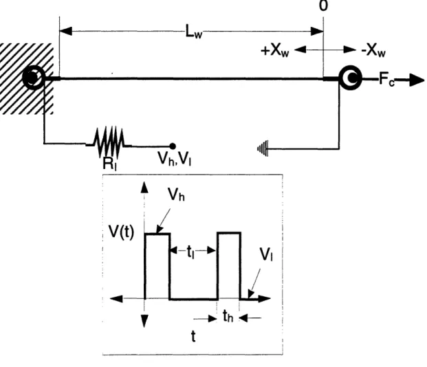
Figure 5. An electrically-heated Ni49Ti51 wire actuating a constant force bias spring.

Figure 5 illustrates a Ni49Ti51 wire under a constant force bias. The position of the wire (Xw) is determined after the constant bias force (Fe) elongates the wire. The wire is electrically heated by the square wave (V). The voltage which heats the wire (Vw) is determined as follows: V,= R V (2) R, + R, I 1 1 I Vl v m r i

I

4-tr-10.

R, is the resulting wire resistance and R, is the load resistor in series with the wire and voltage source. The corresponding wire temperature (Tw(k)) is then determined by applying the discrete form of equation B7. Next, the previous stress in the wire o(k-1) is determined from the previous force in the wire F(k -1).

F(k -1)

a(k-l) = (3)

Aw

The previous stress and actuation cycle (N(k-1)) allow the Ms, Mf, As, Af, unrecovered strain (eu) and shrink loss (SL) to be determined. These allow the resulting temperature strain (&r(k)) to be calculated (see Appendix B). The maximum stress and actuation cycle allow the creep (Ec) in the wire to be calculated. The maximum stress is determined by cycling the wire on the first cycle before any creep can occur. Calculating the wire stiffness (Kw) with equations B 14 through B 16 allows the resulting position of the wire (Xw) to be determined.

Xw(k) = (T(k)- c(k))Lw Fw(k-1) (4) K,

The sign for the contracting temperature strain is positive. The sign for elongating creep is positive. The sign for a bias force which stretches out the wire is positive. The changing length of the wire is finally calculated as follows:

Lw(k)= Li -Xw(k) (5)

Since the bias force is constant for this model, it is not critical to be aware of the previous force being required to calculate various properties of the wire; however, the force is not constant and the lagging estimate is necessary for the next two models.

2.2 Modeling an electrically-heated Ni,4 Tis, wire

actuating a linear bias spring

0

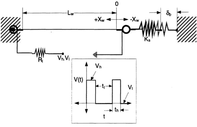
Figure 6. An electrically-heated Ni49Ti51 wire actuating a linear bias spring.

Figure 6 shows the Ni49Ti 51wire actuating a linear bias spring. The variable Ks represents the bias spring stiffness and 8

b represents the net bias distance in the system. The model for the constant force biased Ni49Ti,, wire is used for the linear spring-biased wire; however, the resulting wire position and force require different formulas. The resulting position of the wire is calculated as follows:

Xw (k)[= 1 --SbKs

1

XT (k) = p o [

w

K,

F,(k) = Ks(Xw(k)+Sb) (7)

Using equations 6 and 7 in conjunction with the analysis provided in Section 2.1 completes the model for this system.

2.3 Modeling a bi-stable mechanism employing Ni49Ti51 wires and permanent magnets

L

43

Lce

LJ_

1-~YA~WWZYW77Z

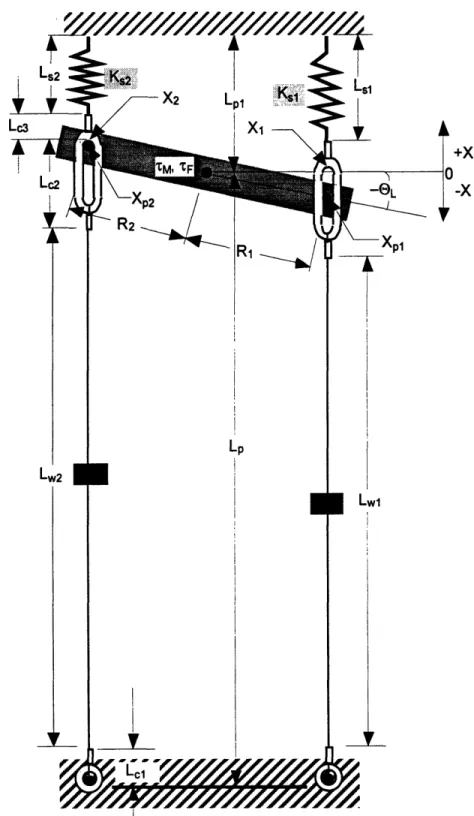
Figure 7. A bi-stable mechanism employing Ni49Ti51 wires and permanent magnets.

VR2

R

Lp

/

n

0

Figure 7 illustrates the bi-stable mechanism employing Ni49Ti51 wires and permanent

magnets. The mechanism consists of two Ni49Ti51 wires biased by two linear springs.

These wires are electrically-heated in the same manner as the linear spring-biased system (a load resistor is still in series with the voltage source). When the wires are electrically heated they contract and move the low-carbon steel lever, which is biased by a permanent magnet pendulum. The magnet pendulum is mounted above the lever in such a way that the angular position of the magnet pendulum is equal to the angular position of the lever. The pendulum is also mounted so that its position is proportional to the angular position (eL) and one-quarter of the length (L) of the steel lever. These assumptions allow the resulting magnetic torque (T,) to be calculated as follows:

TM = 40ma FM (8)

The force of the magnet (FM) varies with angular position because the gap between the steel lever and the permanent magnet increases as the absolute value of the angular position approaches zero. The force will be held constant at the corresponding maximum angular position (Oma). Appendix D describes how to determine the resulting magnetic force for the minimum air gap and magnetic material. In order for the steel not to be saturated by a cylindrical magnet with a diameter (DM), the width (ws) and thickness (ts) need to have the

minimal dimensions:

ws = -2D (9)

ts = " (10)

4

The magnetic and friction torques associated with the lever cause it to accelerate. The resulting lever position (independent of the bounding effects of the actuating wires) can be

determined in the discrete time domain.

When the magnetic torque is positive (clockwise) the following angular position is calculated as follows:

kT2

OL(k)= OL(k-2)+20,(k-1) (T,(k-2)-r,(k-2)) (11)

When the magnetic torque is negative (counterclockwise) the following angular position is calculated as follows:

L(k) kT2

OL(k)= OL(k-2)+20,(k-1)- (Tm,(k-2)-TF,(k-2))

J (12)

The resulting position (X,) in which wire 1 and the connector are pulling the pin of the lever is determined with the following equation:

X, = (Lc, +Lc2-LP)+LwL (13)

In a similar manner the position of wire 2 and its connector (X2) is determined with the following equation:

X2 = (Lc, +Lc2-L,)+LW2 (14)

The changing lengths of wires 1 and 2 (Lwl and LW2) are described by the following equation:

Lw1 = Lw10 + AXW]k - AXTI

LW₂= Lw2o + AW ₂k -

AXT2

(15)

(16)

LwIo and Lw20 are the initial lengths of the wires. AX,, and AXT2 represent the contracted

change in length due to the temperature strain effect. AXWlk and AXW2k represent the

change in the lengths of the two wires resulting from their changing stiffness.

The change in length due to the temperature strain effect is determined by the following equations:

AXTI = (ETI -Ecl)Lw_1o (17)

AX, =(en2-ec2)Lw2o (18)

The temperature strain for wires 1 and 2 (&, and E&) will be determined using the previous determination of the force in the respective wires. The creep for wires 1 and 2 (E-c and Ec2) will be determined using the maximum stress in the wires and the simulation cycle. The change in the wire length due to the changing wire stiffness is determined by the following equations:

FL

)+(L

AX

=

(19)

Kwi

FL is the resulting lever force exerted on either wire 1 or 2. Ks, and KS2 are the

corresponding stiffness for springs 1 and 2. Lc, Lc2 and Lc3 are the corresponding

connector lengths indicated in Figure 7. Ls5 o and Ls2o are the initial lengths for springs 1

and 2. L, and L,, are the respective lengths relative to the pivot pin and the anchors for the wires and springs as indicated in Figure 7. Kw, and KW2 are the changing stiffness for

wires 1 and 2. Ks] and KS2 are the corresponding stiffness for springs 1 and 2. With the

resulting positions of wire 1 and 2 determined, the model needs to determine if the wires are actually pulling each other. This can be determined by using the following check:

if X1 < -X2 + D, then wires are pulling each other

if X1 2 -X2 + D, then wires are not pulling each other

If the wires are pulling each other, they will stretch a given amount (AX,, and AXs2) in order to reach equilibrium. AXs2is determined first as follows:

-(X, +X 2-Dp)

AXs2

=

s2

Z

1+

KW2R2

K,,RI

With AXs2 calculated, AX,, is calculated next:

AXS1 = AXs2 KW2R2 (22)

D, is the diameter of the pins (on the lever) which are in contact with the actuating

connectors for wires 1 and 2. R, and R2 are the corresponding radii from the center of the two pins.

If the wires are pulling each other, then X, and X2 need to be recalculated as follows: X, = XIp ++AX (23)

X2 = X2p +As2 (24)

The forces in wires 1 and 2 (FW, and FW2) are then calculated as follows:

F,, = (AXWk +X s l

)K,, (25)

Fw2 = (AXW2k + AXs2)K ₂ (26)

If the lever pin is in contact with wire 1, the corresponding lever angle is determined as follows:

sin' D]

If the lever pin is in contact with wire 2, the corresponding lever angle is determined as follows:

nX2

OL = sin-' 2 (28)

The lever angle is used to determine the corresponding magnetic torque (t,) and friction torque (IF), which are used to calculate the lever force (F). If the lever is in contact with either wire 1 or 2, then the lever force for the wire in contact is calculated as follows:

FL =

(29)

RI or2

This and the previous two methods discussed will be used to create the computer simulations in Section 3.

3

Computer simulations of SMA-actuated systems

Computer simulations are performed on the SMA-actuated systems modeled in Section 2. Section 3.1 simulates 1 electrically-heated Flexinol 90-110 wire which actuates 4 different constant force bias springs. The wire is simulated in order to compare the theoretical temperature-position results to the experimental results discussed in Appendix C. Section 3.2 simulates a Ni49Ti,5 wire actuating a linear bias spring. The wire is given different manufacturing specifications in the simulation. The simulation illustrates and discusses the dynamic responses of the Ni49Ti5, wire. Section 3.3 simulates a working bi-stable

mechanism employing Ni49Ti51 wires and a permanent magnet pendulum.

3.1 Simulation of an electrically-heated Ni49Ti5, wire

actuating a constant force bias spring

This computer simulation is used to compare the simulated temperature-contraction curves, to the experimental curves discussed in Appendix C. The following parameters for the wire were used in the simulation:

1. Wire type: Flexinol 90-110 wire

* 4250C heat treatment for 1 hour

* pre-cycled 200 times under a 207 MPa stress * temperature strain at As is 0.005

* temperature strain at Af is 0.040 * temperature strain at Mf is 0.005

* temperature strain is zero at To which is 250C

2. Wire dimensions:

* Lwis 61.59 cm * Dw is 75.0 microns

3. Wire stress:

* 4.3 MPa (2 grams or 0.0196 Newtons) * 47.3 MPa (22 grams or 0.2158 Newtons) * 86.0 MPa (40 grams or 0.3924 Newtons) * 150.4 MPa (70 grams or 0.6867 Newtons)

Figures 8 through 11 compare the simulated wire temperature-position curve to the experimental curve. 0.03 0.025 0.02

Xw (m)

Tw (C)

Figure 8. Simulated and experimental temperature-position curves for a 4.3 MPa biased Flexinol 90-110 wire.

Figure 8 indicates that the simulated As temperature is lower than the experimental. It also indicates that the temperature strain may be more than .04 since the experimental wire contracted more than the simulated wire. The unrecovered strain is correct; however, the

lagging recovery could be modeled more accurately to match the actual curve. Despite these differences, as the stress increases in the wires, the simulated and experimental curves tend to match each other more closely.

U.U 0.02. 0.0

Xw (m)

Figure 9. Simulated and experimental temperature-position curves for a 47.3 MPa biased Flexinol 90-110 wire.

Figure 9 indicates that the As temperature is still underestimated. It also indicates that unlike in Figure 8, the strain at Af is overestimated. The simulated Ms temperature

approximately matches the experimental. The unrecovered strain is also correct; however, the lagging recovery could still be modeled. Figures 10 and 11 indicate that the simulated wire results continue to match approximately to the experimental results.

0.03 0.025 0.02

Xw (m)

Tw

(C)

Figure 10. Simulated and experimental temperature-position curves for a 86.0 MPa biased Flexinol 90-110 wire.

Figure 10 indicates that the strain at Af is overestimated. The As temperature is still underestimated. The simulated curve correctly determines that the unrecovered strain should be zero. This simulated curve indicates that the lagging recovery is incorporated in the wire simulation. Figure 11 compares the final temperature-position curves for a 150.4 MPa biased Flexinol 90-110 wire.

0.03 0.025 0.02

Xw (m)

Figure 11. Simulated and experimental temperature-position curves for a 150.4 MPa biased Flexinol 90-110 wire.

Figure 11 indicates that the simulated temperature-position curve closely matches the experimental curve. Figures 8 through 11 indicate that the simulation model provides an adequate means for predicting performance. Section 3.2 simulates an electrically-heated Ni49Ti51wire actuating a linear bias spring, and discusses the dynamic results.

3.2 Simulation of an electrically-heated Ni,4 Tis, wire

actuating a linear bias spring

This computer simulation is used to illustrate the dynamic results of a linear spring-biased wire. A wire is manufactured in the "Create Your Own Wires" menu and is given the following parameters for the simulation:

1. Wire type: Ni₄₉Ti,5

* 4000_{C heat treatment for 1 hour}

* Is not pre-cycled 200 times under a 207 MPa stress * temperature strain at As is .0025

* temperature strain at Af is .05 * temperature strain at Mf is .005

* temperature strain is zero at To which is 250_C

2. Wire dimensions:

SL wis 10 .0 cm

* Dw is 75.0 microns 3. Wire bias spring:

* Ks is 30.0 N/m * 8b iS .008 m 4. Heating parameters: * Tenv is 100

_C

* Rwis18.1192

5. Simulation starts on cycle 10,000

The simulation results are plotted in Figures 12-15:

Figure 12: Simulated temperature-time curve for Ni49Ti51 wire Figure 13: Simulated length-time curve for Ni49Ti51 wire Figure 14: Simulated stress-time curve for Ni49Ti51 wire

Figure 15: Simulated temperature-strain curve for Ni49Ti51 wire

110 100 90 80 70 Tw (C) 60 50 40 30 3n 0 1 2 3 4 5 (seconds)

Figure 12. Simulated temperature-time curve for Ni49Ti51wire.

Figure 12 shows the changing wire temperature as a function of time. The changing temperature corresponds to the heating square wave. The wire temperature repeatedly increases for 1.5 seconds and then decreases for 1.5 seconds. The phase-change effects on

the specific heat are clearly illustrated when the temperature takes .5 seconds to rise from 700_{C to 90}0_{C (the As and Af temperatures). In a similar manner, the temperature takes .4}

seconds to drop from 700_{C to 50}0_{C (the Ms and Mf temperatures). Figure 13 illustrates}

the changing wire length with respect to time.

0.101 0.1 0.099 Lw (m) 0.098 0.097 0.096 (seconds)

Figure 13. Simulated length-time curve for Ni49Ti51wire.

Figure 13 indicates that the wire elongated approximately 1.0 mm (the initial increase in length from .1 to .101 meters) due to creep. As a result, the bias stress in the wire is reduced and the wire is unable to elongate to its initial stretched-out length of .101 meters. Figure 14 displays the corresponding wire stress with respect to time.

8.5 x 10' 8 7.5 7

G (Pa)

Figure 14. Simulated stress-time curve for Ni49Ti51 wire.

Figure 14 illustrates that as the wire elongates, the stress decreases to a point beyond which it can not elongate any further. Due to the amount of creep and type of spring used, the wire was unable to continue elongating once the stress reached 52 MPa. Figure 15 illustrates the resulting temperature-strain curve.

f ," uV. 0.04. 0.0 0.03. 0.0 0.02. ET (m/m) 0.0 0.01r 0.0 0.00. 0 Tw (C)

Figure 15. Simulated temperature-strain curve for Ni49Ti5 wire.

The temperature-strain curve illustrates that the maximum strain has reduced from .05 to .047 after 10,000 cycles. The spring was unable to provide enough bias stress to insure complete elongation of the wire. The strain at As is now .0025. Finally, when the

unrecovered wire's temperature increases, the strain increases in the same manner as if the wire were fully recovered. This final property of the hysteresis loop is unproven;

however, this property is one possible explanation for the inner hysteresis loop. Another explanation could be that the wire does not contract at all until the temperature corresponds to the primary temperature-strain curve. Section 3.3 simulates a working bi-stable

3.3 Simulation of a bi-stable mechanism employing Ni4,Tis, wires and permanent magnets

The bi-stable mechanism simulated in this Section is designed to move the magnet

pendulum back and forth 1,000,000 times. The permanent magnet is Samarium Cobalt and has the following dimensions:

* DM is 5.08 millimeters * LM is 5.08 millimeters

The resulting magnet force (FM) -gap (X,) curve is determined using the formulas and correction factors presented in Appendix D.

FM (I

5x 10 3

(meters)

The minimum gap between the magnet and steel lever is 2.0 mm and the corresponding force is .5 Newtons. The lever length is defined in order to create the magnetic torque (M,)

dependence on the lever's angular position (OL) (see equation 8).

* LL

* Ws

* ts

* Ps

is 5.08 centimeters

is .80 centimeters (see equation 9) is .20 centimeters (see equation 10) is 6,450 kg/m3

-15 -10 -5 0 5 10 15

OL

(degrees)

Figure 17. Resulting magnetic torque-angular position curve from Samarium Cobalt pendulum.

8x 10

(N-(N-m) -R

Friction losses at the rotating pin are neglected; however, the normal friction force (Ff) of the steel lever will be incorporated in simulating any friction losses. The normal friction force is constant at all corresponding lever angles. The friction force, friction radius (Rf), coefficient of static friction (gt) and coefficient of kinetic friction (.k) are chosen as follows:

* Ff is .005 Newtons * Rf is 1.25 centimeters * k, is .30

* Ptk is .10

Two Flexinol 90-110 wires were used with the following dimensions:

* Lw1 is equal to LW2 which is 18.0 centimeters

* DW, is equal to DW2 which is 100 micrometers

The springs which biased the wires have the following stiffness and lengths:

* Ks, is equal to KS2 which is 25 N/m

* Ls, is equal to L S2 which is 5.0 centimeters

The following assembly dimensions are used:

* Lc, is 0.5 centimeters * Lc2 is 2.0 centimeters * Lc3 is 0.5 centimeters SD, is .10 centimeters * R, is 2.0 centimeters * R2 is 2.0 centimeters SL, is 19.9 centimeters * L,, is 8.1 centimeters

The following heating parameters are used for the wires:

* Tev is 250C

* V,, is equal to Vh2 which is 12.0 Volts

* V,, is equal to V₁₂ which is 0.0 Volts

* thl is equal to th2 which is 3.0 seconds * R, is equal to RI2 which is 40.0 Q

* t_c is 4.0 seconds

The following parameters are used to simulate the working system. Figure 18 illustrates the changing angular position of the lever with respect to time.

OL

(degref

0 2 4 6 8 10 12 14 16

t (s)

The resulting angular position is plotted with respect to time. Note that every 4 seconds (ta) one of the wires is being heated. The heated wire is contracting and pulling the lever past 0 degrees in order to allow the magnetic torque to accelerate the lever to the other side. At 0 seconds, wire 1 contracts and pulls the lever past 0 degrees. The lever then accelerates into wire two. At 4 seconds, wire 2 contracts and pulls the lever past 0 degrees, etc. Figure 19 illustrates the corresponding changing stress of wire 2 to the lever position.

Ix 1 o'W2

(Pa)

t(s)

Figure 19. Simulated stress-time curve for Ni49Ti51 wire (wire 2).

As the lever makes contact with wire 2 at 1.5 seconds, the stress increases approximately 40.0 MPa. As the wire begins to contract at 4 seconds, the stress begins to increase. This occurs because the magnetic torque is constant and does not begin to decrease until the absolute value of the angular position is less then 15 degrees. At 4.7 seconds the stress in the wire decreases because the wire force caused by the magnetic torque is decreasing at a faster rate than the spring force is increasing. At approximately 5.5 seconds the lever is no

longer in contact with wire 2 and the stress in the wire is dependent on the bias spring. In Figure 20 the temperature-strain curve for wire 1 is presented.

0.035 0.03 0.025 0.02 ET1

(m/m)

Figure 20. Simulated temperature-strain curve for Ni₄₉Ti55 wire (wire 1).

The temperature-strain curve shows how the strain path from As to Af tends towards the As temperature. This occurs because the stress in the wire decreases for the majority of that transition from As to Af. The As and Af temperatures decrease as the stress decreases;

hence, the slope of the right curve increases as the strain and temperature increase. On the left side of the temperature-strain curve, the slope is constant until the elongating strain is about .0025. At that point the slope becomes less steep because the corresponding Mf temperature has increased. Note that the maximum temperature strain is slightly less than .035. This correctly indicates that after 1,000,000 cycles the wire has lost 12.5% of its net ability to contract.

0

The magnetic force was doubled (increasing the maximum wire stress to 150 MPa). The system was still able to actuate after 1,000,000 cycles. When the magnetic force was tripled (increasing the maximum wire stress to 180 MPa), however, the system could not actuate for 1,000,000 cycles. These simulation results lead to the following general design rules:

1. Design for 3.0% shrink ( 2.0sin(150)/18.0 = .0317 )

2. Note that the remaining 0.5 % shrink will recover from Mf (450C) to To (250C)

3. Bias the wire with 70 MPa stress 4. Maximum actuation stress of 150 MPa

4

Conclusions and Recommendations

A model for Shape Memory Alloys has been presented which addresses the actuating dynamics and the changing properties due to cycling, stress and manufacturing. Thoma's work with the manufacturing and cycling effects on Ni49Ti51 wires enabled a computer

simulation model for these wires to be developed. This computer simulation program approximately matched the experimental temperature-strain curves of Flexinol 90-110 wires. These results imply that the wires were manufactured in the following manner:

1. The Ni49Ti51 wire was first annealed and then cold-worked to reduce the cross-sectional

surface area by 40%.

2. The Ni49Ti51 wire was then heat-treated for 1 hour at 4250C.

3. Next, the Ni49Ti51 wire was constrained with a 4% strain while being cycled 5 times

between the Mf and Af temperatures. This allows the wire to contract and elongate with just a 65 MPa bias stress.

4. Finally, the Ni₄₉Ti51 wire was pre-creeped by cycling the wire approximately 200 times under a 207 MPa stress.

This working model for Ni49Ti51 wires allowed a bi-stable mechanism employing Ni49Ti₅₁

wires and permanent magnets to be simulated. The goal was to make the mechanism cycle 1,000,000 times with pre-creeped Ni49Ti51 wires. The simulation and experimental results led to the following design rules for these wires:

1. Design for 3.0% shrink

2. Note that the remaining 0.5% shrink will recover from Mf (450_{C) to T}

o (250C) 3. Bias the wire with 70 MPa stress

4. Maximum actuation stress of 150 MPa

It is then essential to design the SMA actuating device in such a way so that the maximum strain of the SMA member under stress does not exceed 3% when it transforms to Martensite.

An experimental attempt was made to cycle a Ni49Ti51 wire 1,000,000 times under a 160

MPa stress. Two of the wires cycled approximately 1,000,000 times and two other wires cycled approximately 10,000 times. The cause of wire failure was located at the wire crimp termination. These wire failures imply that any type of constrained bending at the wire's ends will lead to premature failure.

It is essential to prevent localized preferential straining of the actuating member during its transformation from Austenite to Martensite.

-Zhang, Zee and Thoma (1996) A theoretical model was developed to determine the relationship between the resulting permanent magnet pulling force at a given air gap. The model was based on the work done by Fitzgerald (1990), in which a fictitious coil winding is used to drive the flux density of the system to zero in order to determine the coenergy of the magnetic field. Two correction factors were introduced in order to match the theory to the experimental results. The correction factors enable the force-gap curves to be determined for Samarium Cobalt, Neodymium Iron Boron, Bonded Neodymium Iron Boron, Ceramic 5 and Ceramic 8 magnets.

Appendix A:

Users Manual for Design Program

This users manual is written to show how a designer can create the following three simulations:

1. An electrically-heated Ni49Ti51 wire actuating a constant force bias spring. 2. An electrically-heated Ni49Ti51 wire actuating a linear bias spring.

3. A bi-stable mechanism employing Ni49Ti51 wires and permanent magnets.

The design program is written in a higher-level code and requires the software package MATLAB® to operate. The interface occurs in windows with interactive Handle

GraphicsTM objects. The objects which will be used are push buttons, pop-up buttons, and editable-text buttons.

1. Push buttons are used to implement the command displayed on the button. Push buttons can be implemented by moving the mouse pointer over the button and pressing on the mouse button.

2. Pop-up buttons are used to list numerous options to be selected. Pop-up buttons can be implemented by moving the mouse pointer over the button and holding down the mouse button to scroll to a desired selection.

3. Editable-text buttons are used to allow the user to input the desired value for a given variable. Editable-text buttons can be implemented by moving the mouse pointer over the button, depressing the mouse button, and typing the desired text.

A.1 Simulating an electrically-heated Ni49Tis, wire

actuating a constant force bias spring.

V(t)

t

4-Figure Al. An electrically-heated Ni49Ti51 wire actuating a constant force bias spring. Figure Al shows the simulation setup and parameters to be defined by the designer. The designer wants to make a Ni49Ti51 wire, with a given wire length (L,), actuate a constant force (F,) bias spring. The designer needs to create an electrical square wave to heat the wire. The square wave will require high voltage (V,), high time (th), low voltage (V,) and low time (tQ). The designer can also add a load resistor (R,) in series with the Ni49Ti51 wire.

The position of the wire (X,) is set at zero before the constant force bias spring is applied. I

~, ~Ff~in~I GO~1 TO Wire ceFrnceH~sta~ ~ntnten~enpAtr .. ..... . Ajo IN~ .. .... ... eraute$ft4 V T~..n SIM1JLAi

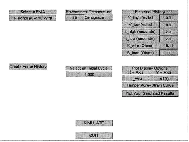
Figure A2. Design menu used to simulate an electrically-heated Ni49Ti₅₁ wire. Figure A2 illustrates the initial design menu to perform the simulation. This menu consists

of six parts:

1. The "Select a SMA" section allows the user to describe the type of Ni49Ti5 1 wire to be

used. There are three choices:

* The "Flexinol 90-110 Wire" choice is for Ni49Ti51 wires manufactured by Dynalloy. The wires have a circular cross-section.

* The "Mondo-tronics Ribbon" choice is for Ni49Tis, _{wires manufactured by} Mondo-tronics. The wires have a rectangular cross-section.

* The "Create Your Own" choice allows the user to manufacture the Ni49Ti,, wire

by choosing options such as the wire's heat treatment temperature, and whether to pre-cycle the wire.

2. The "Environment Temperature" section allows the user to define the environmental temperature.

3. The "Electrical History" section allows the user to define the electrical square wave and load resistance to heat the wire.

4. The "Create Force History" section allows the user to define the constant force bias spring or a linear force bias spring.

5. The "Select an Initial Cycle" section allows the user to define which transformation cycle to simulate. The user can select cycle 1, 10, 100, 1,000, 10,000, 100,000,

1,000,000 or 10,000,000.

6. The "Plot Display Options" section allows the user to plot the simulation results: * time for the simulation (seconds)

* V(t), which is the square wave (Volts) corresponding to time

* T_w(t), which is the wire temperature (Centigrade) corresponding to time * eT(t), which is the temperature strain (m/m) corresponding to time

* X(t), which is the actual position (meters) corresponding to time * Stress(t), which is the wire stress (Pa) corresponding to time * Lw(t), which is the wire length (meters) corresponding to time

:17.Wire Diametersj 75 microns

i

Figure A3. The "Flexinol 90-110 Wires" screen.

Figure A3 shows the resulting window when the "Flexinol 90-110 Wire" choice is made. The length of the wire can be defined. Existing wire diameters of 25, 50, 75, 100, 150 and 250 microns can be chosen. The wires are heat-treated at 4250_{C for 1 hour and pre-cycled}

Figure A4. The "Mondo-tronics Ribbon Wires" screen.

Figure A4 shows the resulting window when the "Mondo-tronics Ribbon" choice is made. The length of the wire can be defined. Existing wire cross-sections of 375 x 2500

microns, and 500 x 2250 microns can be chosen. The wires are heat treated at 4250_{C for 1}

hour and are not pre-cycled. i

1811~11~ ~- L~p~-C-- _~a~B~j

~l~·Bkl~Bsll~-~·lllaC~

Figure A5. The "Create Your Own Wires" screen.

Figure A5 shows the resulting window when the "Create Your Own" choice is made. This screen allows the designer to modify the dimensional, physical and manufacturing

properties of a Ni49Tis' wire. The cross-section can be either circular or rectangular (ribbon wire). The heat-treatment temperature can be either 4000_{C, 425}0_{C or 600}0_{C. The wire can} either be pre-cycled 200 times under a 200 MPa stress, or not be pre-cycled. The

hysteresis curve relating the temperature strain (er) to the wire temperature (T,) can be modified. This modification can be accomplished by defining the temperature strain (r) at the Austenite Start (As), Austenite Finish (Af), and Martensite Finish (Mf) temperatures.

~i~BI I -r I 91F~-- -- I--·C -~' -s~l 111811 ~ls~l~sIlssl~rslllsl~ l~e~l ( ~CIIIPIISqlllllrlll~ II~I~IBl~p ~gL~-- r - rr ~sas~aSSp~a~a

1111~

Figure A6. The "Create Force History" screen (constant force bias option). Figure A6 shows the resulting screen when the designer has selected a constant force bias

spring after selecting the "Create Force History" option from the design menu. Figures A2 through A6 show how the designer could simulate an electrically-heated Ni49Ti51 wire

actuating a constant force bias spring with the following parameters: A Flexinol 90-110 wire with:

* 75 micron diameter * 10.0 centimeter length * 18.11 Ohm wire resistance

The environmental temperature is 100C.

The electrical square wave has the following parameters:

r~lS~B~lB~glB~

mlpipps~4~·pask~sarr

* _{V. is 3.0 Volts for 2.0 seconds (th)} * V, is 0.0 Volts for 2.0 seconds (t,) * The load resistance (R,) is 0 Ohms The constant spring force bias (Fe) was .5 Newtons. Cycle 1,000 was simulated.

A plot of the wire temperature (T_w(t)) on the x-axis and the temperature strain (eT(t)) on the y-axis resulted.

The plotted results were labeled "Temperature-Strain Curve." The curve is plotted in Figure A7. 0.04 0.035 0.03 0.025 0.02 0.015 0.01 0.005 0 Temperature-Strain Curve 0 20 40 60 80 100

Wire Temp (Centigrade)

Figure A7. Simulated temperature-strain curve for Ni49Ti5 1wire.

In a similar manner, the designer can simulate a linear bias springed Ni49Ti5, wire.

A.2 Simulating an electrically-heated Nig4 Tis, wire

actuating a linear bias spring.

O

V(t)

_VI

Figure A8. An electrically-heated Ni49Ti51 wire actuating a linear bias spring. Figure A8 shows the new arrangement when the Ni49Ti51 wire has a linear bias spring.

The information the designer needs to supply is almost identical to the information required for the constant force bias simulation. The new information needed is the spring stiffness

(Ks) and the system bias spring (8_{b). Note that the Ni}

49Ti'S wire position (X,) is based on

its length before it is elongated by the bias spring.

i