HAL Id: inserm-00428524
https://www.hal.inserm.fr/inserm-00428524v2
Submitted on 28 Oct 2009
HAL is a multi-disciplinary open access
archive for the deposit and dissemination of
sci-entific research documents, whether they are
pub-lished or not. The documents may come from
teaching and research institutions in France or
abroad, or from public or private research centers.
L’archive ouverte pluridisciplinaire HAL, est
destinée au dépôt et à la diffusion de documents
scientifiques de niveau recherche, publiés ou non,
émanant des établissements d’enseignement et de
recherche français ou étrangers, des laboratoires
publics ou privés.
Nonlocal means-based speckle filtering for ultrasound
images.
Pierrick Coupé, Pierre Hellier, Charles Kervrann, Christian Barillot
To cite this version:
Pierrick Coupé, Pierre Hellier, Charles Kervrann, Christian Barillot. Nonlocal means-based speckle
filtering for ultrasound images.. IEEE Transactions on Image Processing, Institute of Electrical and
Electronics Engineers, 2009, 18 (10), pp.2221-9. �10.1109/TIP.2009.2024064�. �inserm-00428524v2�
1
NonLocal Means-based Speckle Filtering for
Ultrasound Images
Pierrick Coup´e
1,2,4, Pierre Hellier
1,2,4, Charles Kervrann
3,5and Christian Barillot
1,2,41
University of Rennes I- CNRS UMR 6074, IRISA, Campus de Beaulieu, F-35042 Rennes,France
2INRIA, VisAGeS U746 Unit/Project, IRISA, Campus de Beaulieu, F-35042 Rennes, France
3
INRIA, VISTA Project, IRISA, Campus de Beaulieu, F-35042 Rennes, France
4
INSERM, VisAGeS U746 Unit/Project, IRISA, Campus de Beaulieu, F-35042 Rennes, France
5INRA, UR341 Math´ematiques et Informatique Appliqu´ees, Domaine de Vilvert 78352 Jouy en Josas, France
Abstract
In image processing, restoration is expected to improve the qualitative inspection of the image and the performance of quantitative image analysis techniques. In this paper, an adaptation of the Non Local (NL-) means filter is proposed for speckle reduction in ultrasound (US) images. Originally developed for additive white Gaussian noise, we propose to use a Bayesian framework to derive a NL-means filter adapted to a relevant ultrasound noise model. Quantitative results on synthetic data show the performances of the proposed method compared to well-established and state-of-the-art methods. Results on real images demonstrate that the proposed method is able to preserve accurately edges and structural details of the image.
I. INTRODUCTION
In ultrasound imaging, denoising is challenging since the speckle artifacts cannot be easily modeled and are known to be tissue-dependent. In the imaging process, the energy of the high frequency waves are partially reflected and transmitted at the boundaries between tissues having different acoustic impedances. The images are also log-compressed to make easier visual inspection of anatomy with real-time imaging capability. Nevertheless, the diagnosis quality is often low and reducing speckle while preserving anatomic information is necessary to delineate reliably and accurately the regions of interest. Clearly, the signal-dependent nature of the speckle must be taken into account to design an efficient speckle reduction filter. Recently, it has been demonstrated that image patches are relevant features for denoising images in adverse situations [1]–[3]. The related methodology can be adapted to derive a robust filter for US images. Accordingly, in this paper we introduce a novel restoration scheme for ultrasound (US) images,strongly inspired from the NonLocal (NL-) means approach [1] introduced by Buades et al. [1] to denoise 2D natural images corrupted by an additive white Gaussian noise. In this paper, we propose an adaptation of the NL-means method to a dedicated US noise model [4] using a Bayesian motivation for the NL-means filter [3]. In what follows, invoking the central limit theorem, we will assume that the observed signal at a pixel is a Gaussian random variable with mean zero and a variance determined by the scattering properties of the tissue at the current pixel.
The remainder of the paper is organized as follows. In Section II, we give an overview of speckle filters and related methods. Section III described the proposed Bayesian NL-means filter adapted to speckle noise. Quantitative results on artificial images with various noise models are presented in Section IV. Finally, qualitative result on real 2D and 3D US images are proposed in Section V.
II. SPECKLEREDUCTION:RELATED WORK
The speckle in US images is often considered as undesirable and several noise removal filters have been proposed. Unlike the additive white Gaussian noise model adopted in most denoising methods, US imaging requires specific filters due to the signal-dependent nature of the speckle intensity. In this section, we present a classification of standard adaptive filters and methods for speckle reduction.
A. Adaptive Filters
The adaptive filters are widely used in US image restoration because they are easy to implement and control. The commonly-used adaptive filters - the Lee’s filter [5], Frost’s filter [6], and Kuan’s filter [7] - assume that speckle noise is essentially a multiplicative noise. Many improvements of these classical filters have been proposed since. At the beginning of the 90’s, Lopes et al. [8] suggested to improve the Lee’s and Frost’s filters by classifying the pixels in order to apply specific processing to the different classes. Based on this idea, the so-called Adaptive Speckle Reduction filter (ASR) exploits local image statistics to determine specific areas to be processed further. In [9], the kernel of the adaptive filter is fitted to homogeneous regions according to local image statistics. Analyzing local homogeneous regions was also investigated in [10], [11] to spatially adapt the filter parameters. Note that the Median filter has been also examined for speckle reduction in [4]. Very recently, a stochastic approach to ultrasound despeckling (SBF) has been developed in [12], [13]. This local averaging method removes the local extrema assumed to be outliers in a robust statistical estimation framework. Finally, the Rayleigh-Maximum-Likelihood (R-ML) filter has been derived with similar methodological tools in [14].
B. Partial Differential Equations (PDE) -based approaches
Adapted formulations of the Anisotropic Diffusion filter (AD) [15] and the Total Variation minimization scheme (TV) [16] have been developed for US imaging. In [17], [18], the Speckle Reducing Anisotropic Diffusion (SRAD) was introduced and involves a noise-dependent instantaneous coefficient of variation. In [19] the Nonlinear Coherent Diffusion (NCD) filter is based on the assumption that the multiplicative speckle in US signals is transformed into an additive Gaussian noise in Log-compressed images. Recently, the Oriented SRAD (OSRAD) filter has been proposed in [20]; this filter takes into account the local directional variance of the image intensity, i.e., the local image geometry. Finally, the TV minimization scheme has been adapted to ultrasound imaging in [21], [22]. Unlike the previous adaptive speckle filters, all the considered PDE-based approaches are iterative and produce smooth images while preserving edges. Nevertheless, meaningful structural details are unfortunately removed during iterations.
C. Multiscale methods
Several conventional wavelet thresholding methods [23]–[25] have also been investigated for speckle reduction [26]–[28] with the assumption that the logarithm compression of US images transforms the speckle into an additive Gaussian noise. In order to relax this restrictive assumption, Pizurica et al. [29] proposed a wavelet-based Generalized Likelihood ratio formulation and imposed no prior on noise and signal statistics. In [30]–[33], the Bayesian framework was also explored to perform wavelet thresholding adapted to the non-Gaussian statistics of the signal. Note that other multiscale strategies have been also studied in [34]–[36] to improve the performance of the AD filter; in [37], the Kuan’s filter is applied to interscale layers of a Laplacian pyramid.
D. Hybrid approaches
The aforementioned approaches can be also combined in order to take advantage of the different paradigms. In [38], the image is preprocessed by an adaptive filter in order to decompose the image into two components. A Donoho’s soft thresholding method is then performed on each component. Finally, the two processed components are combined to reduce speckle. PDE-based approaches and a wavelet transform have been also combined as proposed in [39].
III. METHOD
The previously mentioned approaches for speckle reduction are based on the so-called locally adaptive recovery paradigm [40]. Nevertheless, more recently, a new patch-based non local recovery paradigm has been proposed by Buades et al [1]. This new paradigm proposes to replace the local comparison of pixels by the non local comparison of patches. Unlike the aforementioned methods, the so-called NL-means filter does not make any assumptions about the location of the most relevant pixels used to denoise the current pixel. The weight assigned to a pixel in the restoration of the current pixel does not depend on the distance between them (neither in terms of spatial distance nor in terms of intensity distance). The local model of the signal is revised and the authors consider only information redundancy in the image. Instead of comparing the intensity of the pixels, which may be highly corrupted by noise, the NL-means filter analyzes the patterns around the pixels. Basically, image patches are compared for selecting the relevant features useful for noise reduction. This strategy leads to competitive results when compared to most of the state-of-the-art methods [3], [41]–[46]. Nevertheless, the main drawback of this filter is its computational burden. In order to overcome this problem, we have recently proposed a fast and optimized implementation of the NL-means filter for 3D Magnetic Resonance (MR) images [46].
In this section, we rather revise the traditional formulation of the NL-means filter, suited to the additive white Gaussian noise model, and adapt this filter to spatial speckle patterns. Accordingly, a dedicated noise model used for US images is first considered. A Bayesian formulation of the NL-means filter [3] is then used to derive a new speckle filter.
A. The Non Local means Filter
Let us consider a gray-scale noisy image u = (u(xi))xi∈Ωdim defined over a bounded domain Ω
dim ⊂ Rdim, (which is
usually a rectangle of size |Ωdim|) and u(xi) ∈ R+ is the noisy observed intensity at pixel xi∈ Ωdim. In the following, dim
denotes the image grid dimension (dim = 2 or dim = 3 respectively for 2D and 3D images). We also use the notations given below:
Original pixelwise NL-means approach:
∆i : square search volume centered at pixel xi of size |∆i| = (2M + 1)dim, M ∈ N;
Ni : square local neighborhood of xi of size |Ni| = (2d + 1)dim, d ∈ N;
u(Ni) : vector (u(1)(Ni), ..., u(|Ni|)(Ni))T gathering the intensity values of Ni; • v(xi) : true intensity value at pixel xi ∈ Ωdim;
N L(u)(xi) : restored value of pixel xi;
i Nj Ni w (xi,xj) xi xj
Fig. 1. Pixelwise NL-means filter (d = 1 and M = 8). The restored value at pixel xi(in red) is the weighted average of all intensity values of pixels xj
in the search volume ∆i. The weights are based on the similarity of the intensity neighborhoods (patches) u(Ni) and u(Nj).
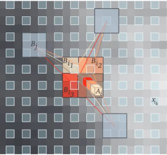
Blockwise NL-means approach:
Bi : square block centered at xi of size |Bi| = (2α + 1)dim, α ∈ N; • v(Bi) : unobserved vector of true values of block Bi;
u(Bi) : vector gathering the intensity values of block Bi;
NL(u)(Bi) : restored block of pixel xi;
w(Bi, Bj) : weight used for restoring u(Bi) given u(Bj) and based on the similarity of blocks u(Bi) and u(Bj).
Finally, the blocks Bik are centered on pixels xik with ik = (k1n, ..., kdimn), (k1, ..., kdim) ∈ N
dim and n represents the
distance between block centers.
1) Pixelwise approach: In the original NL-means filter [1], the restored intensity N L(u)(xi) of pixel xi, is the weighted
average of all the pixel intensities u(xi) in the image Ωdim:
N L(u)(xi) =
X
xj∈Ωdim
w(xi, xj)u(xj) (1)
where w(xi, xj) is the weight assigned to value u(xj) for restoring the pixel xi. More precisely, the weight evaluates the
similarity between the intensities of the local neighborhoods (patches) Ni and Nj centered on pixels xi and xj, such that
w(xi, xj) ∈ [0, 1] and Pxj∈Ωdimw(xi, xj) = 1 (see Fig. 1). The size of the local neighborhood Ni and Nj is (2d + 1)
dim.
The traditional definition of the NL-means filter considers that the intensity of each pixel can be linked to pixel intensities of the whole image. For practical and computational reasons, the number of pixels taken into account in the weighted average is restricted to a neighborhood, that is a “search volume” ∆i of size (2M +1)dim, centered at the current pixel xi.
For each pixel xj in ∆i, the Gaussian-weighted Euclidean distance k.k22,a is computed between the two image patches
u(Nj) and u(Ni) as explained in [1]. This distance is the traditional L2-norm convolved with a Gaussian kernel of standard
deviation a. The standard deviation of the Gaussian kernel is used to assign spatial weights to the patch elements. The central pixels in the patch contribute more to the distance than the pixels located at the periphery. The weights w(xi, xj) are then
computed as follows:
w(xi, xj) =
1 Zi
exp −ku(Ni) − u(Nj)k
2 2,a
h2 (2)
where Zi is a normalization constant ensuring that Pxj∈Ωdimw(xi, xj) = 1, and h acts as a filtering parameter controlling
the decay of the exponential function.
2) Blockwise approach: As presented in [46], a blockwise implementation of the proposed NL-means-based speckle filter is able to decrease the computational burden. The blockwise approach consists of: i) dividing the volume into blocks with overlapping supports; ii) performing a NL-means-like restoration of these blocks; iii)) restoring the pixel intensities from the restored blocks. Here, we describe briefly these three steps and refer the reader to [46] for additional detailed explanations:
i) a partition of the volume Ωdim into overlapping blocks Bik containing P = (2α + 1)
dim elements is performed, i.e.
Ωdim=S
kBik. These blocks are centered on pixels xik which constitute a subset of Ω
dim. The pixels x
ik are equally
distributed at positions ik= (k1n, k2n, k3n), (k1, k2, k3) ∈ Ndim where n represents the distance between the centers of
Bik;
ii) a block Bik is restored as follows:
NL(u)(Bik) = X Bj∈∆ik w(Bik, Bj)u(Bj) with w(Bik, Bj) = 1 Zik
exp −ku(Bik) − u(Bj)k
2 2
B x Bi3 i1 Ai Bj ik Bi2
Fig. 2. Blockwise NL-means Filter (n = 2, α = 1 and L = 4). For each block Bikcentered at pixel xik, a NL-means-like restoration is performed from
blocks Bj. The restored value of the block Bik is the weighted average of all the blocks Bjin the search volume. For a pixel xiincluded in several blocks,
several estimates are obtained and fused. The restored value of pixel xiis the average of the different estimations stored in vector Ai.
where u(Bi) = (u(1)(Bi), ..., u(P )(Bi))T is an image patch gathering the intensities of the block Bi, Zik is a
normal-ization constant ensuringP
Bj∈∆ikw(Bik, Bj) = 1 and ku(Bik) − u(Bj)k 2 2= P X p=1 (u(p)(Bi) − u(p)(Bj))2; (4)
iii) for a pixel xi included in several blocks Bik, several estimates of the same pixel xi from different NL(u)(Bik) are
computed and stored in a vector Ai of size L (see Fig 2). We denote Ai(l) the lth element of vector Ai. The final
restored intensity of pixel xi is the mean of the restored values NL(u)(Bik).
The main advantage of this approach is to significantly reduce the complexity of the algorithm. Indeed, for a volume Ωdim of size |Ωdim|, the global complexity is O((2α + 1)dim(2M + 1)dim(N
n)
dim). For instance, if we set n = 2, the complexity
is divided by a factor of 4 in 2D and 8 in 3D.
B. The NL Means-based Speckle Filter
1) Bayesian formulation: In [3], a Bayesian formulation of the NL-means filter was proposed. Equivalent to the conditional mean estimator, it has been shown that an empirical estimator bv(Bik) of a block Bik can be defined as (see the appendix):
b v(Bik) = 1 |∆ik| |∆ik| X j=1 v(Bj)p(u(Bik)|v(Bj)) 1 |∆ik| |∆ik| X j=1 p(u(Bik)|v(Bj)) (5)
where p(u(Bik)|v(Bj)) denotes the probability density function (pdf) of u(Bik) given the noise free and unknown patches
v(Bj). Since v(Bj) is unknown, an estimator is classically computed by substituting u(Bj) for v(Bj). Hence, we get
b
v(Bik) =
|∆ik|
X
j=1
u(Bj)p(u(Bik)|u(Bj))
|∆ik|
X
j=1
p(u(Bik)|u(Bj))
(6)
where p(u(Bik)|u(Bj)) denotes the pdf of u(Bik) conditionally to u(Bj). In the case of an additive white Gaussian noise,
the likelihood p(u(Bik)|u(Bj)) will be proportional to e
−||u(Bik)−u(Bj )|| 2 2
h2 , and the corresponding Bayesian estimator
b v(Bik)
is then similar to the initial NL-means method (see (3)).
2) Noise models for log-compressed US images: The relevant noise pdfs useful for US image denoising cannot be easily exhibited. Basically, we should consider the complex image formation process, i.e.: i) local correlation due to periodic arrangements of scatterers [17] and finite beamwidth; ii) envelope detection and logarithm amplification of radio-frequency signals performed on the display image [19]; iii) additive Gaussian noise of sensors [19]; iv) additive Gaussian noise introduced by the acquisition card. All these factors tend to prove that the Rayleigh model used for RF signals is not suitable for analyzing US Log-compressed images. Usually, in the wavelet denoising domain [19], [26], [27], multiplicative speckle noise is supposed to be transformed into an additive Gaussian noise by the logarithmic compression. However, recent studies related to US images demonstrate also that the distribution of noise is satisfyingly approximated by a Gamma distribution [47] or a Fisher-Tippett distribution [48].
Consequently, we have decided to choose the following general speckle model:
u(x) = v(x) + vγ(x)η(x) (7) where v(x) is the original image, u(x) is the observed image, η(x)v N (0, σ2) is a zero-mean Gaussian noise. This model is more flexible and less restrictive than the usual RF model and is able to capture reliably image statistics since the factor γ depends on ultrasound devices and additional processing related to image formation.
Contrary to additive white Gaussian noise model, the noise component in (7) is image-dependent. In [4], based on the experimental estimation of the mean versus the standard deviation in Log-compressed images, Loupas et al. have shown that γ = 0.5 model fits better to data than the multiplicative model or the Rayleigh model. Since, this model has been used successfully in many studies [38], [49]–[51]. Clearly, this model is relevant since it is confirmed that the speckle is higher in regions of high intensities versus regions of low intensities [47], [49].
3) A new statistical distance for patch comparison: the Pearson distance: Based on the Bayesian formulation (see (6)), we introduce a new distance to compare image patches if we consider the noise model (7). For each pixel we assume:
u(x)|v(x) v N (v(x), v(x)2γσ2) (8) which yields
p(u(x)|v(x)) ∝ exp −(u(x) − v(x))
2
2v(x)2γσ2 . (9)
Given a block Bi, the likelihood can be factorized as (conditional independence hypothesis):
p(u(Bi)|u(Bj)) = P Y p=1 p(u(p)(xi)|u(p)(xj)) ∝ exp − P X p=1 (u(p)(xi) − u(p)(xj))2 2(u(p))2γ(x j)σ2 . (10)
Accordingly, the so-called Pearson distance defined as
dP(u(Bi), u(Bj)) = P X p=1 (u(p)(Bi) − u(p)(Bj))2 (u(p))2γ(B j) (11)
is substituted to the usual L2-norm (see (4)). In the reminder of the paper, γ = 0.5 is considered in the proposed filter.
A pixel selection scheme similar to [46] based on tests on the mean will be used to select the most relevant patches. This selection is controlled by the thresholding µ1 as previously described in [46]. As a result, the denoising results are improved
and the algorithm is faster. In addition, a parallel implementation is used in all experiments to speed up the algorithm. IV. SYNTHETIC IMAGES EXPERIMENTS
In this section, we propose to compare different filters with experiments on synthetic data, with different noise models, image data and quality criteria. Two simulated data are described in this section:
• in section IV-A, a 2D phantom and a noise model available in MATLAB are considered for the experiments, and the signal-to-noise Ratio (SNR) is used to compare objectively several methods;
• in section IV-B, the realistic speckle simulation proposed in Field II is performed and the ultrasound despeckling assessment index ( eQ) proposed in [12], [13] is chosen for objective comparisons;
Filter iteration number smoothing parameter threshold patch size σ = {0.2; 0.4; 0.8} σ = {0.2; 0.4; 0.8} Lee’s filter - - - 2 × 2 Kuan’s filter - - - 2 × 2 SBF {5; 8; 30} - - 3 × 3 SRAD {500; 1000; 2000} dt = {0.1; 0.2; 0.1} - -NL-means - h = {20.0; 25.0; 30.0} - 5 × 5 OBNLM - h = {12.0; 14.0; 16.0} µ1= 0.9 5 × 5 TABLE I
OPTIMAL SET OF PARAMETERS USED FOR THE MATLAB“PHANTOM”EXPERIMENT. FOR THENL-meansBASED FILTERS,WE SETn = 2AND
|∆ik| = 11 × 11.
A. 2D phantom corrupted by the theoretical (MATLAB) noise model
1) Speckle model and quality criterion: In this experiment, the synthetic image “Phantom” (see Fig. 3), available inMATLAB, was corrupted with different levels of noise. The “Phantom” image is a 32 bit image of 256 × 256 pixels. First, an offset of 0.5 was added to the image (to avoid naught areas) before performing a multiplication of intensities by a factor 20. Then, the
MATLABspeckle simulation based on the following image model
u(xi) = v(xi) + v(xi)ν(xi), ν(xi) v N (0, σ2) (12)
was applied to the “Phantom” image. Three levels of noise were tested by setting σ = {0.2; 0.4; 0.8}. To assess denoising methods, the SNR values [52] were computed between the “ground truth” and the denoised images :
SN R = 10 log10 P xi∈Ω2(v(xi) 2+ b v(xi)2) P xi∈Ω2(v(xi) −v(xb i)) 2 (13)
where v(xi) is the true value of pixel xi andbv(xi) the restored intensity of pixel xi.
2) Compared methods: In this experiment, we compared several speckle filters and the parameters were adjusted to get the best SNR values:
• Lee’s filter (2D MATLAB implementation) [5]
• Kuan’s filter (2D MATLAB implementation) [7]
• SBF filter (2D MATLABimplementation provided by the authors) [12]
• Speckle Reducing Anisotropic Diffusion (SRAD) (MATLABimplementation of Virginia University1) [17]
• blockwise implementation of the classical NL-means filter [1]
• blockwise implementation of the proposed method denoted as Optimized Bayesian NL-means with block selection (OBNLM).
In this experiment, we have chosen to compare our method with well-known adaptive filters, such as the Lee’s and Kuan’s filters, and with two competitive state-of-the-art methods: SRAD and SBF filters. We limited the comparison to this set of methods but the results produced by other recent filters could be also analyzed further (e.g. see [14]). Moreover, the usual NL-means filter has been applied to the same images in order to quantitatively evaluate the performance of our speckle-based NL-means filter. For each method and for each noise level, the optimal filter parameters were searched within large ranges. These parameters are given in Table I.
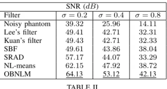
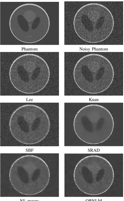
3) Results: Table II gives the SNR values obtained for each method. The denoised images corresponding to σ = 0.4 are presented in Fig. 3. For all levels of noise, the OBNLM filter obtained the best SNR value. For this experiment, the use of the Pearson distance combined with block selection enabled to improve the denoising performances of the NL-means filter for images corrupted by signal-dependent noise. Visually, the NL-means based filter satisfyingly removed the speckle while preserving meaningful edges.
B. Field II simulation
1) Speckle model and quality assessment: In order to evaluate the denoising filters with a more relevant and challenging simulation of speckle noise, the validation framework proposed in [12], [13] was used. This framework is based on Field II simulation [53]. The “Cyst” phantom is composed of 3 constant classes Cr presented in Fig. 4. The result of the Field II
simulation is converted into an 8 bit image of size 390 × 500 pixels. Since the geometry of the image is known, but not the true value of the image (i.e. without speckle), the authors introduced the ultrasound despeckling assessment index ( eQ) defined as:
SNR (dB) Filter σ = 0.2 σ = 0.4 σ = 0.8 Noisy phantom 39.32 25.96 14.11 Lee’s filter 49.41 42.71 32.31 Kuan’s filter 49.43 42.71 32.33 SBF 49.61 43.86 38.04 SRAD 57.17 44.07 33.29 NL-means 62.15 47.92 38.72 OBNLM 64.13 53.12 42.13 TABLE II
SNRVALUES OBTAINED WITH SEVERAL FILTERS APPLIED TO THE2DMATLAB“PHANTOM”IMAGE.
Filter iteration number smoothing parameter threshold patch size
SBF 400 - - 5 × 5
SRAD 500 dt = 0.05 - -NL-means - h = 50 - 11 × 11
OBNLM - h = 50 µ1= 0.75 11 × 11
TABLE III
OPTIMAL SET OF PARAMETERS USED FOR VALIDATION ON THE2DSYNTHETIC DATA SIMULATED WITHFIELDII. FOR THENL-means-BASED FILTERS
n = 4AND|∆ik| = 33 × 33. Q = P r6=l(µCr− µCl) 2 P rσ 2 Cr (14) to evaluate the performance of denoising filters for this simulation. We denote µCr as the mean and σ
2
Cr as the variance of
class Cr after denoising. To avoid the sensitivity to image resolution, Q is normalized by Qid. The new index eQ = Q/Qid
is high if the applied filter is able to produce a new image with well separated classes and small variances for each class. According to [12], [13], an image is satisfyingly denoised if eQ is high enough.
2) Method Comparison: For this experiment, we compared the SBF filter, SRAD filter, NL-means filter and the proposed OBNLM filter. The filter parameters are given in Table III. Compared to the previous experiment, the patch size by using the NL-means-based filters is increased. Indeed, the patch size reflects the scale of the “noise” compared to the image resolution. In the previous experiment, the resolution of the added noise was about one pixel. In this experiment, the objects to be removed are composed of several pixels, thus the patch size is increased to evaluate the restoration performance of each object.
3) Results: The denoised images and the quantitative results are given in Fig. 4. In this evaluation framework, the OBNLM filter produced the highest eQ index. Similar values than those presented in [12], [13] were found for the SRAD and SBF filters. Compared to the original NL-means filter, the proposed adaptations for US images improved the eQ index of the denoised image.
V. EXPERIMENTS ON REAL DATA
In this section, a visual comparison of 2D intraoperative ultrasound brain images (Section V-A) and a visual inspection of 3D ultrasound image of a liver (Section V-B) are proposed.
A. Intraoperative ultrasound brain images
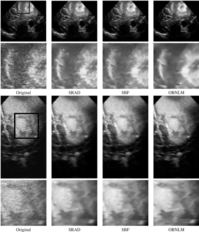
In this paragraph, we propose a visual comparison of the SBF and SRAD filters and the OBNLM method on real intraoperative brain images. The parameters for the SBF and SRAD filters are the parameters given respectively in [17] and [12]. The parameters of the OBNLM filter were set as follows : h = 8, n = 2, α = 3, M = 6 and µ1= 0.6.
Figure 5 shows the denoising results. Visually, the OBNLM filter efficiently removes the speckle component while enhancing the edges and preserving the image structures. The visual results produced on real image by our method are competitive compared to SRAD and SBF filters.
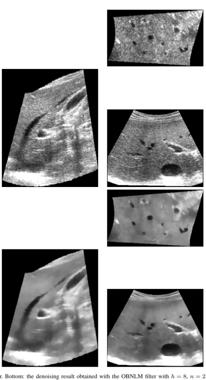
B. Experiments on a 3D liver image
In this section, result of the proposed filter on 3D US image is proposed. These data are freely available on Cambridge University website2. The B-scans were acquired with a Lynx ultrasound unit (BK Medical System) and tracked by the magnetic
tracking system miniBIRD (Ascension Technology). The reconstruction of the volume was performed with the method described in [54]. The reconstructed volume size was 308 × 278 × 218 voxels with an isotropic resolution of 0.5 × 0.5 × 0.5 mm3.
The denoising results obtained with the OBNLM method on the liver volume are shown in Fig. 6. As for the previous experiment on 2D US brain images, the visual results on this 3D dataset show edge preservation and efficient noise removal produced by our filter.
Phantom Noisy Phantom
Lee Kuan
SBF SRAD
NL-means OBNLM
Fig. 3. Results obtained with different filters applied to the “Phantom” image corrupted with signal-dependent noise (σ = 0.4). The quantitative evaluation, measured using the signal-to-noise ratio, is presented in Table II.
Figure 7 shows zooming views of hepatic vessels. The edge preservation of the OBNLM filter is visible on the removed noise image that does not contain structures. Moreover, the difference in dark areas (hepatic vessels) and gray areas (hepatic tissues) shows the smoothing adaptation according to the signal intensity. The noise in brighter areas is drastically reduced.
VI. CONCLUSION
In this paper, we proposed a Non Local (NL)-means-based filter for ultrasound images by introducing the Pearson distance as a relevant criterion for patch comparison. Experiments were carried out on synthetic images with different simulations of speckle. During the experiments, quantitative measures were used to compare several denoising filters. Experiments showed that the Optimized Bayesian Non Local Means (OBNLM) filter proposes competitive performances compared to other state-of-the-art methods. Moreover, as assessed by quantitative results, our adaptation of classical NL-means filter to speckle noise proposes a filter more suitable for US imaging. Experiments on real ultrasound data were conducted and showed that the OBNLM method is very efficient at smoothing homogeneous areas while preserving edges. Further work will be pursued on the automatic tuning of the OBNLM filter and on the influence study on post-processing tasks such as image registration or image segmentation.
ACKNOWLEDGMENT
The authors thank Peter Tay for providing the MATLAB code of the SBF filter. The authors thank the reviewers for their fruitful comments.
Cyst Field II simulation
SRAD eQ = 2.11 SBF eQ = 2.27
NL-means eQ = 1.95 OBNLM eQ = 2.71
Fig. 4. Denoised images obtained with the compared filters for the Field II experiment and the corresponding ˜Q indexes.
APPENDIX
Details of the Bayesian NL-means filter
The following Bayesian definition of the NL-means filter is presented in [3]. By considering the quadratic loss function, the optimal Bayesian estimator of a noise-free patchvbopt(B) can be written as:
b vopt(B) = argmin v(B) X v(B) ||v(B) −bv(B)||2p(v(B)|u(B)) = X v(B) v(B)p(v(B)|u(B)) (15)
where p(v(B)|u(B)) denotes the probability density function (pdf) of v(B) conditionally to u(B), u(B) is the observed intensity and v(B) is the true intensity of block B. According to the Bayes’ and marginalization rules, the so-called conditional mean estimator can be rewritten as (see [3]) :
b vopt(B) = X v(B)p(v(B)|u(B)) p(u(B)) = P v(B)v(B)p(u(B)|v(B))p(v(B)) P v(B)p(u(B)|v(B))p(v(B)) (16)
where p(u(B)|v(B)) denotes the distribution of u(B) conditionally to v(B). Since p(u(B)|v(B)) and p(u(v)) cannot be estimated from only one realization of the image, these pdfs are estimated from observations (blocks Bj) taken in a search
window ∆i of a block Bi. According to [3], [55], the following approximations can be written:
1 |∆i| |∆i| X j=1 v(Bj)p(u(Bi)|v(Bj)) P −→P v(B)v(B)p(u(B)|v(B))p(v(B)) (17) 1 |∆i| |∆i| X j=1 p(u(Bi)|v(Bj)) P −→P v(B)p(u(B)|v(B))p(v(B)), (18)
If we assume the prior distribution p(v(B)) uniform. This leads to the empirical Bayesian estimatorv(Bb ik) uses in (5):
b v(Bi) = 1 |∆i| |∆i| X j=1 v(Bj)p(u(Bi)|v(Bj)) 1 |∆i| |∆i| X j=1 p(u(Bi)|v(Bj)) . (19)
We refer the reader to [3] for detailed explanations.
REFERENCES
[1] A. Buades, B. Coll, and J. M. Morel, “A review of image denoising algorithms, with a new one,” Multiscale Modeling & Simulation, vol. 4, no. 2, pp. 490–530, 2005.
[2] S. P. Awate and R. T. Whitaker, “Unsupervised, information-theoretic, adaptive image filtering for image restoration,” IEEE Trans. Pattern Anal. Mach. Intell., vol. 28, no. 3, pp. 364–376, 2006.
[3] C. Kervrann, J. Boulanger, and P. Coup´e, “Bayesian non-local means filter, image redundancy and adaptive dictionaries for noise removal,” in Proc. Conf. Scale-Space and Variational Meth. (SSVM’ 07), Ischia, Italy, June 2007, pp. 520–532.
[4] T. Loupas, W. McDicken, and P. Allan, “An adaptive weighted median filter for speckle suppression in medical ultrasound image,” IEEE T. Circ. Syst., vol. 36, pp. 129–135, 1989.
[5] J. S. Lee, “Digital image enhancement and noise filtering by use of local statistics,” IEEE Transactions on Pattern Analysis and Machine Intelligence, vol. 2, pp. 165–168, 1980. [Online]. Available: http://adsabs.harvard.edu/cgi-bin/nph-bib query?bibcode=1980ITPAM...2..165L
[6] V. Frost, J. Stiles, K. Shanmugan, and J. Holtzman, “A model for radar images and its application to adaptive digital filtering of multiplicative noise,” IEEE Transactions on Pattern Analysis and Machine Intelligence, vol. 2, pp. 157–65, 1982.
[7] D. Kuan, A. Sawchuck, T. Strand, and P.Chavel, “Adaptive noise smoothing filter for images with signal-dependent noise,” IEEE Transactions on Pattern Analysis and Machine Intelligence, vol. 7, no. 2, pp. 165–177, 1985.
[8] A. Lopes, R. Touzi, and E. Nezry, “Adaptive speckle filters and scene heterogeneity,” IEEE Transactions on Geoscience and Remote Sensing, vol. 28, pp. 992–1000, 1990.
[9] M. Karaman, M. A. Kutay, and G. Bozdagi, “An adaptive speckle suppression filter for medical ultrasonic imaging,” IEEE Transactions on Medical Imaging, vol. 14, no. 2, pp. 283–292, 1995. [Online]. Available: http://ieeexplore.ieee.org/xpls/abs\ all.jsp?arnumber=387710
[10] E. Kofidis, S. Theodoridis, C. Kotropoulos, and I. Pitas, “Nonlinear adaptive filters for speckle suppression in ultrasonic images,” Signal Processing, vol. 52, no. 3, pp. 357–72, 1996. [Online]. Available: citeseer.ist.psu.edu/kofidis96nonlinear.html
[11] J. M. Park, W. J. Song, and W. A. Pearlman, “Speckle filtering of sar images based on adaptive windowing,” Vision, Image and Signal Processing, vol. 146, no. 4, pp. 191–197, 1999. [Online]. Available: http://ieeexplore.ieee.org/xpls/abs all.jsp?arnumber=803320
[12] P. C. Tay, S. T. Acton, and J. A. Hossack, “A stochastic approach to ultrasound despeckling,” in Biomedical Imaging: Nano to Macro, 2006. 3rd IEEE International Symposium on, 2006, pp. 221–224. [Online]. Available: http://ieeexplore.ieee.org/xpls/abs\ all.jsp?arnumber=1624892
[13] ——, “Ultrasound despeckling using an adaptive window stochastic approach,” in IEEE International Conference on Image Processing, 2006, pp. 2549–2552. [Online]. Available: http://ieeexplore.ieee.org/xpls/abs\ all.jsp?arnumber=4107088
[14] T. C. Aysal and K. E. Barner, “Rayleigh-maximum-likelihood filtering for speckle reduction of ultrasound images,” IEEE Transactions on Medical Imaging, vol. 26, no. 5, pp. 712–727, 2007. [Online]. Available: http://ieeexplore.ieee.org/xpls/abs all.jsp?arnumber=4162627
[15] P. Perona and J. Malik, “Scale-space and edge detection using anisotropic diffusion,” IEEE Transactions on Pattern Analysis and Machine Intelligence, vol. 12, no. 7, pp. 629–639, 1990.
[16] L. Rudin, S. Osher, and E. Fatemi, “Nonlinear total variation based noise removal algorithms,” Physica D, vol. 60, pp. 259–268, 1992. [17] Y. Yu and S. T. Acton, “Speckle reducing anisotropic diffusion,” IEEE Transactions on Image Processing, vol. 11, no. 11, pp. 1260–1270, 2002. [18] Y. Yu, J. A. Molloy, and S. T. Acton, “Three-dimensional speckle reducing anisotropic diffusion,” in Signals, Systems and Computers,
2003. Conference Record of the Thirty-Seventh Asilomar Conference on, vol. 2, 2003, pp. 1987–1991 Vol.2. [Online]. Available: http://ieeexplore.ieee.org/xpls/abs\ all.jsp?arnumber=1292329
[19] K. Z. Abd-Elmoniem, A. B. Youssef, and Y. M. Kadah, “Real-time speckle reduction and coherence enhancement in ultrasound imaging via nonlinear anisotropic diffusion.” IEEE Transactions on Biomedical Engineering, vol. 49, no. 9, pp. 997–1014, 2002. [Online]. Available: http://www.ncbi.nlm.nih.gov/entrez/query.fcgi?cmd=Retrieve\&db=pubmed\&dopt=Abstract\&list uids=12214889
[20] K. Krissian, C. F. Westin, R. Kikinis, and K. G. Vosburgh, “Oriented speckle reducing anisotropic diffusion,” IEEE Transactions on Image Processing, vol. 16, no. 5, pp. 1412–1424, 2007. [Online]. Available: http://ieeexplore.ieee.org/xpls/abs all.jsp?arnumber=4154795
[21] C. Sheng, Y. Xin, Y. Liping, and S. Kun, “Total variation-based speckle reduction using multi-grid algorithm for ultrasound images,” in ICIAP: international conference on image analysis and processing, vol. 3617, 2005, pp. 245–252.
[22] K. Djemal, “Speckle reduction in ultrasound images by minimazation of total variation,” in ICIP: international conference on image processing, vol. 3, 2005, pp. 357–360.
[23] D. Donoho and I. Johnstone, “Ideal spatial adaptation by wavelet shrinkage,” Biometrika, vol. 81, no. 3, pp. 425–455, 1994. [24] D. Donoho, “De-noising by soft-thresholding,” IEEE Transactions on Information Theory, vol. 41, no. 3, pp. 613–627, 1995.
[25] R. Coifman and D. Donoho, “Translation invariant de-noising,” in in Lecture Notes in Statistics: Wavelets and Statistics, New York, February 1995, pp. 125–150.
[26] J. E. Odegard, H. Guo, M. Lang, C. S. Burrus, R. O. Wells, L. M. Novak, and M. Hiett, “Wavelet based SAR speckle reduction and image compression,” in SPIE Proc. on Algorithms for Synthetic Aperture, vol. 2487, 1995, pp. 259–271.
[27] L. Gagnon and D. F. Smaili, “Speckle noise reduction of airborne sar images with symmetric daubechies wavelets,” in Proc. SPIE Signal and Data Processing of Small Targets, O. E. Drummond, Ed., vol. 2759, 1996, pp. 14–24. [Online]. Available: http: //adsabs.harvard.edu/cgi-bin/nph-bib query?bibcode=1996SPIE.2759...14G
[28] X. Zong, A. F. Laine, and E. A. Geiser, “Speckle reduction and contrast enhancement of echocardiograms via multiscale nonlinear processing,” IEEE Transactions on Medical Imaging, vol. 17, no. 4, pp. 532–540, 1998. [Online]. Available: http://ieeexplore.ieee.org/xpls/abs\ all.jsp?arnumber=730398 [29] A. Pizurica, , A. M. Wink, E. Vansteenkiste, W. Philips, and J. Roerdink, “A review of wavelet denoising in mri and ultrasound brain imaging,”
Current Medical Imaging Reviews, vol. 2, no. 2, pp. 247–260, 2006. [Online]. Available: http://dx.doi.org/10.2174/157340506776930665
[30] A. Achim, A. Bezerianos, and P. Tsakalides, “Novel bayesian multiscale method for speckle removal in medical ultrasound images,” IEEE Transactions on Medical Imaging, vol. 20, pp. 772–783, Aug. 2001. [Online]. Available: citeseer.comp.nus.edu.sg/484966.html
[31] S. Foucher, G. B. Benie, and J. M. Boucher, “Multiscale map filtering of sar images,” IEEE Transactions on Image Processing, vol. 10, no. 1, pp. 49–60, 2001. [Online]. Available: http://ieeexplore.ieee.org/xpls/abs\ all.jsp?arnumber=892442
[32] S. Gupta, R. C. Chauhan, and S. C. Saxena, “Locally adaptive wavelet domain bayesian processor for denoising medical ultrasound images using speckle modelling based on rayleigh distribution,” Vision, Image and Signal Processing, IEEE Proceedings -, vol. 152, no. 1, pp. 129–135, 2005. [Online]. Available: http://ieeexplore.ieee.org/xpls/abs\ all.jsp?arnumber=1408933
[33] M. I. H. Bhuiyan, Omair, and M. N. S. Swamy, “New spatially adaptive wavelet-based method for the despeckling of medical ultrasound images,” in IEEE International Symposium on Circuits and Systems, 2007. ISCAS 2007., 2007, pp. 2347–2350. [Online]. Available: http://ieeexplore.ieee.org/xpls/abs\ all.jsp?arnumber=4253146
[34] Z. Yang and M. D. Fox, “Speckle reduction and structure enhancement by multichannel median boosted anisotropic diffusion,” EURASIP J. Appl. Signal Process., vol. 2004, no. 1, pp. 2492–2502, January 2004. [Online]. Available: http://portal.acm.org/citation.cfm?id=1289549
[35] O. Acosta, H. Frimmel, A. Fenster, and S. Ourselin, “Filtering and restoration of structures in 3d ultrasound images,” in Biomedical Imaging: From Nano to Macro, 2007. ISBI 2007. 4th IEEE International Symposium on, 2007, pp. 888–891. [Online]. Available: http://ieeexplore.ieee.org/xpls/abs\ all.jsp?arnumber=4193429
[36] F. Zhang, Y. M. Yoo, L. M. Koh, and Y. Kim, “Nonlinear diffusion in laplacian pyramid domain for ultrasonic speckle reduction,” IEEE Transactions on Medical Imaging, vol. 26, no. 2, pp. 200–211, 2007. [Online]. Available: http://ieeexplore.ieee.org/xpls/abs\ all.jsp?arnumber=4077869
[37] B. Aiazzi, L. Alparone, and S. Baronti, “Multiresolution local-statistics speckle filtering based on a ratio laplacian pyramid,” IEEE Transactions on Geoscience and Remote Sensing, vol. 36, no. 5, pp. 1466–1476, 1998. [Online]. Available: http://ieeexplore.ieee.org/xpls/abs\ all.jsp?arnumber=718850 [38] X. Hao, S. Gao, and X. Gao, “A novel multiscale nonlinear thresholding method for ultrasonic speckle suppressing.” IEEE Transactions on Medical Imaging, vol. 18, no. 9, pp. 787–794, 1999. [Online]. Available: http://www.ncbi.nlm.nih.gov/entrez/query.fcgi?cmd=Retrieve\&db=pubmed\&dopt= Abstract\&list uids=10571383
[39] A. Ogier, P. Hellier, and C. Barillot, “Restoration of 3D medical images with total variation scheme on wavelet domains (TVW),” in SPIE Medical Imaging, vol. 6144, February 2006.
[40] M. Elad, “On the origin of the bilateral filter and ways to improve it.” IEEE Transactions on Image Processing, vol. 11, no. 10, pp. 1141–1151, 2002. [41] C. Kervrann and J. Boulanger, “Optimal spatial adaptation for patch-based image denoising,” IEEE Transactions on Image Processing, vol. 15, no. 10,
2006.
[42] S. Kindermann, S. Osher, and P. W. Jones, “Deblurring and denoising of images by nonlocal functionals,” Multiscale Modeling & Simulation, vol. 4, no. 4, pp. 1091–1115, 2005.
[43] H. Q. Luong, A. Ledda, and W. Philips, “Non-local image interpolation,” in IEEE International Conference on Image Processing, 2006, pp. 693–696. [Online]. Available: http://ieeexplore.ieee.org/xpls/abs all.jsp?arnumber=4106624
[44] T. Brox and D. Cremers, “Iterated nonlocal means for texture restoration,” in Proc. International Conference on Scale Space and Variational Methods in Computer Vision, ser. LNCS. Ischia, Italy: Springer, May 2007.
[45] C. Kervrann and J. Boulanger, “Local adaptivity to variable smoothness for exemplar-based image regularization and representation,” International Journal of Computer Vision, 2008, accepted for future publication. [Online]. Available: http://dx.doi.org/10.1007/s11263-007-0096-2
[46] P. Coup´e, P. Yger, S. Prima, P. Hellier, C. Kervrann, and C. Barillot, “An Optimized Blockwise NonLocal Means Denoising Filter for 3-D Magnetic Resonance Images,” IEEE Transactions on Medical Imaging, vol. 27, no. 4, pp. 425–441, April 2008.
[47] Z. Tao, H. D. Tagare, and J. D. Beaty, “Evaluation of four probability distribution models for speckle in clinical cardiac ultrasound images,” IEEE Transactions on Medical Imaging, vol. 25, no. 11, pp. 1483–1491, 2006. [Online]. Available: http://ieeexplore.ieee.org/xpls/abs all.jsp?arnumber=1717646 [48] G. Slabaugh, G. Unal, T. Fang, and M. Wels, “Ultrasound-specific segmentation via decorrelation and statistical region-based active contours,” in IEEE
Computer Society Conference on Computer Vision and Pattern Recognition, vol. 1, 2006, pp. 45–53.
[49] K. Krissian, K. Vosburgh, R. Kikinis, and C.-F. Westin, “Speckle-constrained anisotropic diffusion for ultrasound images,” in IEEE Computer Society Conference on Computer Vision and Pattern Recognition, June 2005.
[50] F. Argenti and G. Torricelli, “Speckle suppression in ultrasonic images based on undecimated wavelets,” EURASIP Journal on Advances in Signal Processing, vol. 2003, no. 5, pp. 470–478, 2003.
[51] M. P. Wachowiak, A. S. Elmaghraby, R. Smol´ıkova, and J. M. Zurada, “Classification and estimation of ultrasound speckle noise with neural networks.” in IEEE International Symposium on Bio-Informatics and Biomedical Engineering (BIBE’00), 2000, pp. 245–252.
[52] D. Sakrison, “On the role of the observer and a distortion measure in image transmission,” IEEE Transactions on Communications, vol. 25, no. 11, pp. 1251–1267, 1977. [Online]. Available: http://ieeexplore.ieee.org/xpls/abs\ all.jsp?arnumber=1093773
[53] J. A. Jensen, “Field: A program for simulating ultrasound systems,” Medical & Biological Engineering & Computing, vol. 34, pp. 351–353, 1996. [54] P. Coup´e, P. Hellier, X. Morandi, and C. Barillot, “Probe Trajectory Interpolation for 3D Reconstruction of Freehand Ultrasound,” Medical Image
Analysis, vol. 11, no. 6, pp. 604–615, 2007.
[55] F. Godtliebsen, E. Spjotvoll, and J. S. Marron, “A nonlinear gaussian filter applied to images with discontinuities,” J. Nonparametr. Statist., vol. 8, no. 1, pp. 21–43, 1997. [Online]. Available: http://dx.doi.org/10.1080/10485259708832713
Original SRAD SBF OBNLM
Original SRAD SBF OBNLM
Fig. 5. Results obtained with the SRAD and SBF filters and the proposed filters on real intraoperative brain images. The OBNLM filter efficiently removes the speckle while enhancing the edges and preserving the image structures.
Fig. 6. Top: 3D volume of the liver. Bottom: the denoising result obtained with the OBNLM filter with h = 8, n = 2, α = 1, M = 5 and µ1= 0.6.
Fig. 7. From left to right: the original “noisy” volume, the denoising result obtained with the OBNLM filter with h = 8 and µ1= 0.6 and the removed
noise component. The edge preservation of the OBNLM is visually appreciated by inspecting the removed noise component which contains few structures. Moreover, the level of noise estimated for the dark areas (hepatic vessels) and the gray areas (hepatic tissues) demonstrates the relevance of the signal-dependent modeling.