Publisher’s version / Version de l'éditeur:
Vous avez des questions? Nous pouvons vous aider. Pour communiquer directement avec un auteur, consultez la
première page de la revue dans laquelle son article a été publié afin de trouver ses coordonnées. Si vous n’arrivez pas à les repérer, communiquez avec nous à [email protected].
Questions? Contact the NRC Publications Archive team at
[email protected]. If you wish to email the authors directly, please see the first page of the publication for their contact information.
https://publications-cnrc.canada.ca/fra/droits
L’accès à ce site Web et l’utilisation de son contenu sont assujettis aux conditions présentées dans le site LISEZ CES CONDITIONS ATTENTIVEMENT AVANT D’UTILISER CE SITE WEB.
ASCE International Conference on Pipeline Engineering and Construction [Proceedings], pp. 1-12, 2004-08-01
READ THESE TERMS AND CONDITIONS CAREFULLY BEFORE USING THIS WEBSITE. https://nrc-publications.canada.ca/eng/copyright
NRC Publications Archive Record / Notice des Archives des publications du CNRC :
https://nrc-publications.canada.ca/eng/view/object/?id=34583cf7-bbcd-41f9-9a53-280ed8240e52 https://publications-cnrc.canada.ca/fra/voir/objet/?id=34583cf7-bbcd-41f9-9a53-280ed8240e52
NRC Publications Archive
Archives des publications du CNRC
This publication could be one of several versions: author’s original, accepted manuscript or the publisher’s version. / La version de cette publication peut être l’une des suivantes : la version prépublication de l’auteur, la version acceptée du manuscrit ou la version de l’éditeur.
Access and use of this website and the material on it are subject to the Terms and Conditions set forth at
Modeling failure risk in buried pipes using fuzzy Markov deterioration process
Modeling failure risk in buried pipes using fuzzy Markov deterioration process
Kleiner, Y.; Sadiq, R.; Rajani, B.
NRCC-46739
A version of this document is published in / Une version de ce document se trouve dans : ASCE International Conference on Pipeline Engineering and Construction,
San Diego, CA., August 2-4, 2004, pp. 1-12
Modeling failure risk in buried pipes using fuzzy Markov deterioration
process
1*
Yehuda Kleiner, 2Rehan Sadiq, and 1Balvant Rajani
ABSTRACT: Numerous models have been proposed in the last two decades for the
deterioration of buried pipes. The most prominent approach has been the Markovian deterioration processes (MDP), which requires that the condition of the deteriorating system be encoded as an ordinal condition state. This encoding is based on numerous distress indicators obtained possibly from direct and indirect observations, as well as from non-destructive tests. To date, few buried pipes have been inspected and their condition assessed. In addition, the encoding of distress indicators into condition states is inherently imprecise and involves subjective judgment. Furthermore, the consequences of failure for buried pipes are often difficult to quantify precisely due to lack of data.
In this paper, a new approach is presented to model the deterioration of buried pipes using a fuzzy rule-based, non-homogeneous Markov process. This deterioration model yields possibility of failure at every point along the life of the pipe. The possibility of failure, expressed as a fuzzy number, is coupled with the failure consequence (also expressed as a fuzzy number) to obtain the failure risk as a function of the pipe age. The use of fuzzy sets and fuzzy techniques help to incorporate the inherent imprecision and subjectivity of the data, as well as to propagate these attributes throughout the model, yielding more realistic results. At the time of submission, adequate and sufficient data to validate the model were not available.
1 Introduction
Large buried pipes typically have low failure rates but when they fail the
consequences can be quite severe. This low rate of failure, coupled with high cost of inspection and condition assessment, have contributed to the current situation where most municipalities lack the data necessary to model the deterioration rates of these assets and subsequently to make rational decisions regarding their renewal.
The condition assessment of a large buried pipe comprises two steps. The first step involves the inspection of the pipe using direct observation (visual, video) and/or non-destructive evaluation (NDE) techniques (radar, sonar, ultrasound, sound emissions, eddy currents, etc.), which reveal distress indicators. The second step involves the interpretation of these distress indicators to determine the condition state of the pipe. This interpretation process is dependent upon the inspection technique. The interpretation of the visual inspection results, although based on strict guideline, can often be influenced by subjective judgment. The interpretation of NDE results on the other hand, is often complex (at times proprietary) and imprecise.
1
Senior Research Officer Institute for Research in Construction (IRC), National Research Council Canada (NRC)
2
Research Officer Institute for Research in Construction, National Research Council Canada * corresponding author
Managing the failure risk of large buried pipes requires a deterioration model to enable the forecast of the asset condition as well as its possibility of failure in the future. Significant research effort has been carried out in the last two decades to model infrastructure deterioration. The Markov deterioration process (MDP) is one approach that has gained prominence as exemplified by Madanat et al. (1997), Li et
al. (1997), Abraham and Wirahadikusumah (1999), Wirahadikusumah et al. (2001),
Mishalani and Madanat (2002), Kleiner (2001) and others. Examples of other types of statistical models include Lu and Madanat (1994), Ramia and Ali (1997), Flourentzou
et al. (1999), Ariaratnam et al. (2001) and others.
In recent years increased research effort has been dedicated to the application of soft computing methods to assess infrastructure deterioration. Soft computing methods include techniques such as artificial neural network (ANN), genetic algorithms (GA), belief networks (BN), fuzzy sets and fuzzy techniques. Fuzzy techniques seem to be particularly suited to model the deterioration of infrastructure assets for which data are scarce and cause-effect knowledge is imprecise. Some examples from the literature of various applications of fuzzy techniques to infrastructure systems include: Chao and Cheng (1998) used a fuzzy-based pattern recognition model to diagnose cracks in reinforced concrete structures; Liang et al. (2001) developed a multiple-layer fuzzy method for concrete bridge health monitoring; Sadiq et al. (2004) employed a fuzzy-based technique for determining the soil corrosivity as a surrogate for breakage/corrosion rate in cast iron pipes..
2 Fuzzy
sets
A fuzzy set describes the relationship between an uncertain quantity x and a
membership function µ, which ranges between 0 and 1. A fuzzy set is an extension of the traditional set theory (in which x is either a member of set A or not) in that an x can be a member of set A with a certain degree of membership µ. Fuzzy techniques help address deficiencies inherent in binary logic and are useful in propagating uncertainties through models. A general definition of a fuzzy set is given by Dubois and Prade (1985): if x is a member of set Ai with a certain degree of membership µAi(x), denoted as Ai = {(x, µAi(x))}, then Ai is a fuzzy set if x takes its value from the
real numbers line and µAi(x) ∈ [0, 1].
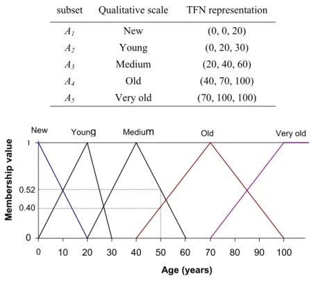
The proposed models use triangular fuzzy numbers (TFN), as these are often used for representing linguistic variables (Lee, 1996). To illustrate the concept, suppose that the age of a pipe is defined by five fuzzy subsets (or numbers), each representing an aging grade; A1 = “new”, A2 = “young”, A3 “medium”, A4 = “old” and
A5 = “very old”, as illustrated in Figure 1. The fuzzy subset A3 “medium” for
example, has a membership function such that for age x below 20 years or above 60 years the membership to “medium” is zero, and for age between 20 and 60 years the membership follows straight lines that form a triangle. Fuzzy set A comprises the collection of the five subsets (or numbers) Ai. The fuzzy subsets Ai are triangular
fuzzy numbers that can be defined by three points representing the three vertices of the respective triangle, as shown in Figure 1.
In this example, it can be seen that for a pipe of age x = 50 years the membership values are µA3(x) = 0.40, and µA4(x) = 0.52 and zeros for µA1(x) µA2(x) and µA5(x). The
5-tuple fuzzy set representing the buried pipe at age 50 can be written as the vector
A = (µA1(x), µA2(x), µA3(x), µA4(x), µA5(x)) = (0, 0, 0.40, 0.52, 0), in which each
element (tuple) depicts the pipe’s membership value to the corresponding subset of aging grade (from new to very old).
There is a whole range of arithmetic operations defined for triangular fuzzy numbers Details of these arithmetic manipulations are described by Klir and Yuan (1995). The term “defuzzification” refers to a process to evaluate a crisp or point estimate of a fuzzy number. A defuzzified value is generally represented by a centroid, often determined using the center of area method (Yager, 1980).
subset Qualitative scale TFN representation
A1 New (0, 0, 20) A2 Young (0, 20, 30) A3 Medium (20, 40, 60) A4 Old (40, 70, 100) A5 Very old (70, 100, 100) 0.40 0.52 Very old Old Medium 1 Young New 0 Memb er sh ip valu e 10 20 100 0 30 40 50 60 70 80 90 Age (years)
Figure 1. Example of fuzzy sub-sets (numbers).
3
The fuzzy rule-based algorithm
In fuzzy rule-based modeling, the relationships between variables are represented by means of fuzzy if-then rules of the form “If antecedent proposition then consequent proposition”. The antecedent proposition is always a fuzzy proposition of the type “x is A” where x is a linguistic variable and A is a linguistic constant term. The
proposition’s truth-value (a real number between zero and 1) depends on the degree
of similarity between x and A. This linguistic model (Mamdani, 1977) has the capacity to capture qualitative and highly uncertain knowledge in the form of if-then rules such as
Ri: If x is Aj then y is Bk; i = 1, 2, …, L; j = 1, 2, …, M; k = 1, 2, …, N (1)
(2)
(3) where x is the input (antecedent) linguistic variable and Aj is an antecedent linguistic
constant. (one of M in set A) Similarly, y is the output (consequent) linguistic variable and Bk is a consequent linguistic constant (one of N in set B). The values of x and y,
and Aj and Bk are fuzzy sets defined in the domains of their respective base variables.
The linguistic terms Aj and Bk are selected from sets of predefined terms, such as small, medium, large. The rule set (comprising L rules) and the sets A and B
constitute the knowledge base of the linguistic model. Each rule is regarded as a fuzzy relation: Ri (X × Y) → [0, 1]. This relation can be computed in two basic ways -
by using fuzzy implications or fuzzy conjunctions, (Mamdani method), which were used in the proposed model. There are several steps involved in the Mamdani method, as described in Mamdani (1977) and in relevant textbooks, e.g., Yager and Filov (1994). The entire procedure can be summarized as
y = x o R
which means that if the rule set R is established, then for every input x, output y can be calculated (or inferred) using the appropriate operator “o”. A fuzzy set can be “defuzzified”, i.e. assigned a representative crisp value. There are several techniques in the literature for defuzzification, but the one used here is the most widely accepted technique known as the centroidal method (Yager, 1980).
The Mamdani inference algorithm can be extended to multiple inputs and single output (MISO):
Ri: If x1 is A1j and x2 is A2j and….and xp is Apj then y is Bk
4
Fuzzy rule-based Markovian deterioration process (FR-MDP)
4.1 The knowledge base
Figure 2 depicts the knowledge base for the proposed deterioration model. The age A of the pipe is partitioned into 5 levels (from new to very old), represented by triangular fuzzy subsets Ai (i = 1,2,…,5), with underlying units of years. Similarly, the condition C of the pipe is partitioned into 7 levels (from excellent to failed) represented by
triangular fuzzy subsets Ci (i = 1,2,…,7). C is mapped onto an arbitrary unitless
relative scale in the interval [0,1]. It should be noted that the failed state does not mean that collapse has already occurred (in which case the membership would be a clear unity), rather that it is imminent. The deterioration rate D’ is partitioned into 5 levels (from very slow to very fast) represented by triangular fuzzy subsets D’i (i = 1,2,…,5). D’ is mapped onto a dynamic relative scale with underlying units of membership per
MLV- :most likely value
Ri = If pipe age (A) is “A” and pipe condition state (C) is “C” then deterioration rate (D) is “D’” (at time = t)
Pipe condition (C): Excellent Good Adequate Fair Poor Bad Failed
Age (A): New Slow Average Fast Very fast Very fast Very fast Very fast Young Slow Average Fast Fast Fast Very fast Very fast Medium Very slow Slow Average Average Fast Fast Very fast Old Very slow Very slow Slow Slow Average Average Fast Very old Very slow Very slow Very slow Slow Slow Average Average
Knowledge-base
Deterioration rate Min MLV Max
Very slow 0 0 d0 Slow 0 d0 2d0 Average d0 2d0 3d0 Fast 2d0 3d0 4d0 Very fast 3d0 4d0 4d0 Very fast Average Fast Very slow 0 d0 2d0 3d0 4d0 Me mbe rship µD = 1.0 Slow
Deterioration rate (membership shifted/year) Condition state Min MLV Max
Excellent 0 0 0.17 Good 0 0.17 0.33 Adequate 0.17 0.33 0.50 Fair 0.33 0.50 0.67 Poor 0.50 0.67 0.83 Bad 0.67 0.83 1 Failed 0.83 1 1
Age Min MLV Max
New 0 0 20
Young 0 20 40
Medium 20 40 70
Old 40 70 100
Very old 70 100 100
Age of the pipe (A, years)
Very old Old Young Medium New 0 20 40 60 80 100 Me mbe rship µA = 1.0 Bad
Pipe condition state (C, qualitatively defined)
Fair Good Exce-llent Me mbe rship µC = 1.0
Adeq-uate Poor Failed
0.83 0.33
0 0.17 0.50 0.67 1
Fuzzy rule-set RD
Figure 2. Fuzzy rule-base for the Markovian deterioration process (FR-MDP)
year. The base deterioration rate parameter d0, (Figure 2 – Deterioration rate chart) is
found through regression as is later explained. The typical range of the deterioration scale will usually be between zero and 0.2 membership per year.
The table at the bottom of Figure 2 depicts the set of fuzzy rules RD governing this
model. For example, if the asset age is A= young and its condition is C = fair then its deterioration rate is D’ = fast. The rule set RD thus contains 35 fuzzy rules.
4.2 The deterioration process
The deterioration process is modeled as a “flow” of membership from one condition state to the next lower condition state. The deterioration in each time step comprises two steps. In the first step, the pipe age is fuzzified (mapped on A). The pipe’s fuzzy condition state at time step (taken for convenience as a single year) t is Ct. The fuzzy
deterioration at t, D’t is computed using the Mamdani (1977) algorithm detailed
earlier for the MISO model – equation (3) where At and Ct are the inputs, D’t is the
output and RD is the fuzzy rule-set by which the fuzzy inferences are made.
D’t = (At ^ Ct) o RD (4)
(5)
D’t, is a 5-tuple fuzzy set which is then defuzzified using the center of mass method.
The defuzzified (crisp) value of the fuzzy deterioration D’t is denoted by Dt. In the
second step, the condition of the asset in the next time step Ct+1 is calculated from its
condition state in the current time step Ct and the (defuzzified) deterioration rate Dt
obtained by rule-based algorithm in the current time step as follows
Ct+1 = Ct⊗ Dt
where Ct is the condition at year t, Dt is the deterioration rate estimated by fuzzy rule
set from At and Ct and ⊗ is an operator. The exact nature of this operator is discussed
in detail in Kleiner et al. (2004). In essence it controls the “flow” of membership from one condition state to a more deteriorated condition state.
In traditional Markov deterioration models it is quite possible that at any time step t, significant memberships (or probabilities) in more that 3 conditions states can results. This outcome would be contrary to intuitive expert opinion. This situation is
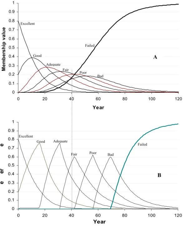
remedied by introducing threshold values, which restrict the membership “flow” from one condition state to the next. Figure 3 illustrates an example in which deterioration models with and without thresholds are compared. At t = 40 years for example, the condition state of the pipe in the model without threshold is approximately
C40 = {0, 0.09, 0.16, 0.17, 0.20, 0.21, 0.17}, which means that the pipe has relatively
significant membership value =0.09 to state 2 (good) and membership value =0.17 to state 7 (failed) simultaneously. This is of course un-realistic. In contrast, the model with threshold yields C
2 C µ 7 C µ 40 = {0, 0.09, 0.36, 0.54, 0, 0, 0}, which is much
more realistic. Membership to the failed state (state 7) at any given time t can be viewed as the possibility (not probability) of failure at that time.
In order to train the model to an existing asset one needs to know (or assume) the condition state of the asset immediately after installation, and at least one condition assessment at a later age t. The model is trained by minimizing the sum of square deviations between the observed and predicted membership values for time t. The
val u sh ip mb M 0 0.1 0.2 0.3 0.4 0.5 0.6 0.7 0.8 0.9 1 0 20 40 60 80 100 120 Year M em b er sh ip val u e 0 0.1 0.2 0.3 0.4 0.5 0.6 0.7 0.8 0.9 1 0 20 40 60 80 100 120 Year e er e B A Failed Bad Poor Fair Adequate Good Excellent Failed Bad Poor Fair Adequate Good Excellent
Figure 3. Deterioration curves without (A) and with (B) membership thresholds. parameters that vary in the training process are those controlling the scale and shape of the deterioration fuzzy set, namely do and the aforementioned threshold values.
In order to validate the proposed model, one needs at least two consecutive
observations of the asset condition. Further, these observations need to be reasonably distant (in time) from each other, to avoid errors due to small inconsistencies due to the subjective nature of the condition assessment of an asset. The first observation is needed to train the model and predict future deterioration, whereas the second
observation is required to evaluate the prediction. Unfortunately, the data required for model validation were not available, making the validation of the model impossible.
4.3 Fuzzy possibility of failure
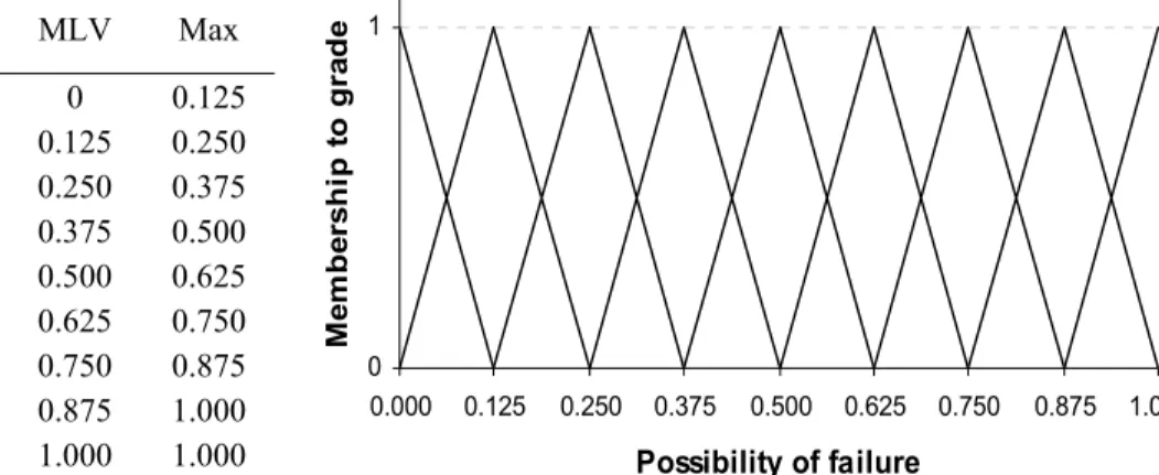
Fuzzy sets, such as TFNs are often interpreted as possibility distributions (in contrast to probability distribution) (Klir and Yuan, 1995). It follows that the membership value to the failed condition can be viewed as the possibility of failure. These membership values can be mapped onto a secondary fuzzy scale, comprising nine grades from extremely low to extremely high, as illustrated in Figure 4.
*Qualitative
scale Min MLV Max
Extremely low 0 0 0.125 Very low 0 0.125 0.250 Quite low 0.125 0.250 0.375 Moderately low 0.250 0.375 0.500 Medium 0.375 0.500 0.625 Moderately high 0.500 0.625 0.750 Quite high 0.625 0.750 0.875 Very high 0.750 0.875 1.000 Extremely high 0.875 1.000 1.000 0 1 0.000 0.125 0.250 0.375 0.500 0.625 0.750 0.875 1.000 Possibility of failure M e m b er sh ip to g rad e
Figure 4. Fuzzy possibility of failure
5 Fuzzy
rule-based
risk
Lawrence (1976) defines risk it as a measure of probability and severity of negative
adverse effects. When a complex system involves various contributory risk items with
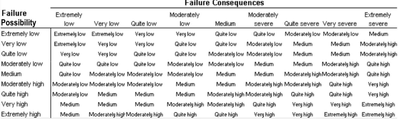
uncertain sources and magnitudes, it often cannot be treated with mathematical rigor during the initial or screening phase of decision-making (Lee, 1996). In the realm of buried pipes failures, not only is the likelihood of failure difficult to quantify, but failure consequences as well. Consequently, consequences of failure will be defined on a fuzzy qualitative nine-grade scale from extremely low to extremely severe. A fuzzy rule-based MISO model is proposed for the risk analysis. The inputs to the model are the fuzzy possibility of failure, which is used in lieu of probability of failure, and fuzzy failure consequences. The output is risk level, which is also
partitioned into 9 levels from extremely low to extremely high. The fuzzy rule-set (81 rules in total) is shown in Figure 5.
Possibility
Figure 5. Rule-base for fuzzy risk
For example, immediately after installation a pipe is assumed to have been in a condition state represented by the fuzzy set C0 = (0.9, 0.1, 0, 0, 0, 0, 0) meaning 0.9
membership to excellent and 0.1 membership to good. At age 30 years an inspection and condition assessment was carried out and the pipe’s condition was determined to be C30 = (0, 0.2, 0.7, 0.1, 0, 0, 0) meaning 0.2 membership to good, 0.7 membership
to adequate and 0.1 membership to fair. After a regression analysis, the resulting deterioration curves are as illustrated in Figure 6 below.
Figure 6. Example deterioration curves 0.1 0.2 0.3 0.4 0.5 0.6 0.7 0.8 0.9 1 M e mb er sh ip val u e Failed Bad Poor Fair Adequate Good Excellent 0 0 20 40 60 80 100 120 Year
For each year, t, in the life of the pipe, the membership to condition failed is re-mapped onto a fuzzy set depicting the possibility of failure (Figure 4).
Next, a pipe-failure consequence is arbitrarily (for this example) assumed to be represented by the fuzzy set S = (0, 0, 0, 0, 0, 0.2, 0.5, 0.3, 0), meaning membership
values of 0.2, 0.5 and 0.3 to fuzzy subsets moderately severe, quite severe, and very
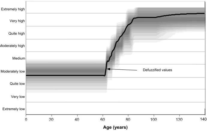
severe respectively. The resulting fuzzy risk curve is illustrated in Figure 7. The
intensity of the gray levels represents the membership values to the respective risk levels. The black curve represents the defuzzified risk values. It can be seen that the defuzzified values do not always coincide with the highest membership values, which means that the fuzzy set representing risk at any year t is not always symmetrical about its mode.
0 20 40 60 80 100 120 14014 0 20 40 60 80 100 120 140 Defuzzified values Age (years) Medium Moderately low Moderately high Quite high Quite low Very low Very high Extremely high Extremely low
Figure 7. Fuzzy risk levels over the life of a pipe
4. Summary
The scarcity of data about the deterioration rates of buried infrastructure assets, coupled with the imprecise and often subjective nature of assessment of pipe
condition merits the usage of fuzzy techniques in modeling the deterioration of these assets. The deterioration process is modeled as a fuzzy rule-based non-homogeneous Markov process applied at each time step in two stages. In the first stage, the
deterioration rate at the specific time step is inferred from the asset age and condition state using a fuzzy rule-base algorithm. In the next stage, the condition state of the pipe is calculated from present condition state and deterioration rate. Essentially as the deterioration process progresses, the pipe gradually “flows” from higher membership in good condition states to higher membership in worse states. The process is formulated to mimic the reality in which a given asset at a given time
cannot have significant membership values to more than two or three different (and consecutive) condition states.
The deterioration model is trained by non-linear regression in which the sum of square deviations between predicted and observed membership values is minimized. Data were not available to validate this model, but this should not deter water utilities from using it, as the model provides a framework for collecting the appropriate data, which would be required to validate any model. The model can be used to predict the future deterioration rate of the asset, subject to some judgment-based assumptions. Once deterioration curves are obtained, the membership value to the failed state is viewed as the possibility of failure and is mapped onto a secondary fuzzy scale with nine failure possibility grades ranging from extremely low to extremely high. The consequences of pipe failure are defined on a fuzzy scale with nine intensity grades ranging from extremely low to extremely severe. The level of risk, which is also defined on a nine-grade fuzzy scale from extremely low to extremely high, can then be determined (inferred) based on a fuzzy rule base.
Acknowledgement
This paper presents interim results of an on-going research project, which is co-sponsored by the American Water Works Association Research Foundation
(AwwaRF), the National Research Council of Canada (NRC) and water utilities from the United States, Canada and Australia.
References
Abraham, D.M., and Wirahadikusumah, R. 1999. Development of prediction model for sewer deterioration, Proceedings of the 8th Conference Durability of Building Materials and Components, Edited by M.A. Lacasse and D.J. Vanier, NRC, pp.
1257-1267, Vancouver.
Ariaratnam, S.T., A. El-Assaly, and Y. Yang. 2001. Assessment of infrastructure needs using logistic models, Journal of Infrastructure Systems, ASCE, 7(4): 160-165. Chao, C-J., and Cheng, F.P. 1998. Fuzzy pattern recognition model for diagnosing
cracks in RC structures, Journal of Computing in Civil Engineering, ASCE, 12(2): 111-119.
Dubois, D., and Prade, H. 1985. Evidence measures based on fuzzy information,
Automatica, 21(5): 547-562.
Flourentzou, F., E. Brandt, and C. Wetzel. 1999. MEDIC – a method for predicting residual service life and refurbishment investment budgets, Proceedings of the 8th
conference Durability of Building Materials and Components, Edited by M.A.
Lacasse and D.J. Vanier, IRC, NRC, pp. 1280-1288, Vancouver.
Kleiner, Y. 2001. Scheduling inspection and renewal of large infrastructure assets,
Journal of Infrastructure Systems, ASCE, 7(4): 136-143.
Kleiner, Y. Sadiq, R., and Rajani, B.B. 2004. Modeling the deterioration of buried infrastructure as a fuzzy Markov process, Submitted toJournal of Infrastructure Systems, ASCE.
Klir, G.J., and Yuan, B. 1995. Fuzzy sets and fuzzy logic - theory and applications, Prentice- Hall, Inc., Englewood Cliffs, NJ, USA.
Lawrence, W.W. 1976. Of acceptable risk, William Kaufmann, Los Altos, CA. Lee, H.-M. 1996. Applying fuzzy set theory to evaluate the rate of aggregative risk in
software development, Fuzzy Sets and Systems, 79: 323-336.
Li, N., Haas, L.R., and Xie, W-C. 1997. Development of a new asphalt pavement
performance prediction model, Canadian Journal of Civil Engineering, 24: 547-559. Liang, M.T., Wu, J.H., and Liang, C.H. 2001. Multiple layer fuzzy evaluation for
existing reinforced concrete bridges, Journal of Infrastructure Systems, ASCE, 7(4): 144-159.
Lu, Y., and S.M. Madanat. 1994. Bayesian updating of infrastructure deterioration models, Transportation Research Record, 1442: 110-114.
Madanat, S.M., Karlaftis, M.G., and McCarthy, P.S. 1997. Probabilistic infrastructure deterioration models with panel data, Journal of Infrastructure Systems, ASCE, 3(1): 4-9.
Mishalani, R.G., and S.M. Madanat. 2002. Computation of infrastructure transition probabilities using stochastic duration models, Journal of Infrastructure Systems,
ASCE, 8(4): 139-148.
Madanat, S.M., Mishalani, R., and Wan Ibrahim, W.H. 1995. Estimation of infrastructure transition probabilities from condition rating data, Journal of
Infrastructure Systems, ASCE, 1(2): 120-125.
Mamdani, E.H. 1977. Application of fuzzy logic to approximate reasoning using linguistic systems, Fuzzy Sets and Systems, 26: 1182-1191.
Ramia, A.P., and N. Ali. 1997. Bayesian methodologies for evaluating rutting in Nova Scotia’s special B asphalt concrete overlays, Canadian Journal of Civil
Engineering, 24(4): 1-11.
Sadiq, R., Rajani, B.B. and Kleiner, Y. 2004. A fuzzy based method of soil corrosivity evaluation for predicting water main deterioration, Submitted to
Journal of Infrastructure Systems, ASCE.
Wirahadikusumah, R., Abraham, D., and Isely, T. 2001. Challenging issues in modeling deterioration of combined sewers”, Journal of Infrastructure Systems,
ASCE, 7(2): 77-84.
Yager, R.R. 1980. A general class of fuzzy connectives, Fuzzy Sets and Systems, 4: 235-242.
Yager, R.R., and Filev, D.P. 1994. Essentials of fuzzy modeling and control, John Wiley & Sons, Inc., NY.