HAL Id: hal-00299235
https://hal.archives-ouvertes.fr/hal-00299235
Submitted on 1 Aug 2005
HAL is a multi-disciplinary open access
archive for the deposit and dissemination of
sci-entific research documents, whether they are
pub-lished or not. The documents may come from
teaching and research institutions in France or
abroad, or from public or private research centers.
L’archive ouverte pluridisciplinaire HAL, est
destinée au dépôt et à la diffusion de documents
scientifiques de niveau recherche, publiés ou non,
émanant des établissements d’enseignement et de
recherche français ou étrangers, des laboratoires
publics ou privés.
”Montserrat-2000” flash-flood event using statistical and
deterministic methods
S. Mariani, M. Casaioli, C. Accadia, M. C. Llasat, F. Pasi, S. Davolio, M.
Elementi, G. Ficca, R. Romero
To cite this version:
S. Mariani, M. Casaioli, C. Accadia, M. C. Llasat, F. Pasi, et al.. A limited area model
intercompar-ison on the ”Montserrat-2000” flash-flood event using statistical and deterministic methods. Natural
Hazards and Earth System Science, Copernicus Publications on behalf of the European Geosciences
Union, 2005, 5 (4), pp.565-581. �hal-00299235�
SRef-ID: 1684-9981/nhess/2005-5-565 European Geosciences Union
© 2005 Author(s). This work is licensed under a Creative Commons License.
and Earth
System Sciences
A limited area model intercomparison on the “Montserrat-2000”
flash-flood event using statistical and deterministic methods
S. Mariani1, M. Casaioli1, C. Accadia1, M. C. Llasat2, F. Pasi3, S. Davolio4, M. Elementi5, G. Ficca6, and R. Romero7
1Agenzia per la Protezione dell’Ambiente e per i Servizi Tecnici, APAT, Rome, Italy
2Departament d’Astronomia i Meteorologia, Facultat de F´ısica, Universitat de Barcelona, Barcelona, Spain 3Laboratorio di Meteorologia e Modellistica Ambientale, LaMMA, Sesto Fiorentino, Florence, Italy 4CNR-Istituto di Scienze dell’Atmosfera e del Clima, CNR-ISAC, Bologna, Italy
5Agenzia Regionale Prevenzione e Ambiente dell’Emilia-Romagna, Servizio Idro Meteo, ARPA-SIM, Bologna, Italy 6Servizio Agrometeorologico Regionale per la Sardegna, SAR, Sassari, Italy
7Departament de F´ısica, Universitat de les Illes Balears, Palma de Mallorca, Spain
Received: 2 February 2005 – Revised: 20 April 2005 – Accepted: 3 May 2005 – Published: 1 August 2005 Part of Special Issue “HYDROPTIMET”
Abstract. In the scope of the European project
Hydropti-met, INTERREG IIIB-MEDOCC programme, limited area model (LAM) intercomparison of intense events that pro-duced many damages to people and territory is performed. As the comparison is limited to single case studies, the work is not meant to provide a measure of the different models’ skill, but to identify the key model factors useful to give a good forecast on such a kind of meteorological phenom-ena. This work focuses on the Spanish flash-flood event, also known as “Montserrat-2000” event.
The study is performed using forecast data from seven op-erational LAMs, placed at partners’ disposal via the Hydrop-timet ftp site, and observed data from Catalonia rain gauge network. To improve the event analysis, satellite rainfall es-timates have been also considered.
For statistical evaluation of quantitative precipitation fore-casts (QPFs), several non-parametric skill scores based on contingency tables have been used. Furthermore, for each model run it has been possible to identify Catalonia regions affected by misses and false alarms using contingency table elements. Moreover, the standard “eyeball” analysis of fore-cast and observed precipitation fields has been supported by the use of a state-of-the-art diagnostic method, the contigu-ous rain area (CRA) analysis. This method allows to quantify the spatial shift forecast error and to identify the error sources that affected each model forecasts.
High-resolution modelling and domain size seem to have a key role for providing a skillful forecast. Further work is needed to support this statement, including verification using a wider observational data set.
Correspondence to: S. Mariani
1 Introduction
Intense hydro-meteorological events can be the cause of many different risk conditions for society and territory. Ad-vances in the forecasting capabilities and increased under-standing of such phenomena can be achieved by the op-timization of the current hydro-meteorological forecasting techniques. In particular, a strong exchange among determin-istic case-study research, real-time monitoring of local obser-vation data and the use of statistical and diagnostic method-ologies for forecasting model validation and intercomparison is required.
In this context, the activity of the EU project Hydropti-met (INTERREG IIIB-MEDOCC programme) had as focal points the improvement of the hydro-meteorological fore-casting methodologies and the knowledge exchange among project partners. With these objectives in mind, four case studies of intense hydro-meteorological events, which af-fected in the recent past the north-western Mediterranean area causing many damages, have been selected. In fact, these events, which had different physical and meteorolog-ical characteristics, had been chosen to perform an intercom-parison study using the numerical model forecasts available at partners’ centers.
Among the four selected case studies, this work focuses on the “Montserrat-2000” flash-flood event occurred on 9– 10 June 2000 in northeastern Iberian Peninsula (Llasat et al., 2003). The case study has been chosen for its characteris-tics: a flash-flood event due to a mesoscale Mediterranean cyclone, with primary role played by the mesoscale forcing mechanisms typically acting in the Mediterranean Basin (dy-namical forcing enhanced by orography and wet processes).
Precipitation forecast fields of seven hydrostatic and non-hydrostatic limited area models (LAMs) have been compared
Fig. 1. Catalonia (Spain) internal basins (from Llasat et al., 2003).
with the precipitations observed at Catalonia rain gauge sta-tions. The selected models have different horizontal grid size, ranging from 2 km to 10 km. As the intercompari-son results could be affected by the grid size differences, a remapping procedure (Accadia et al., 2003; Baldwin, 2000) has also been applied to perform an intercomparison on a common 10-km grid. This grid-to-grid transformation has been preferred to other techniques, since it conserves, to a desired degree of accuracy, the total forecast precipitation of the native grid.
Model validation, both in a statistical (i.e., non-parametric skill scores; contingency table element analysis) and in a deterministic (i.e., “eyeball” verification, quantitative com-parison of observed and forecast fields over hydrological basins; object-oriented analysis) approach, has been per-formed. Such a single-case investigation could provide in-sight on physical mechanisms related to forecast errors, thus giving hints about eventual drawbacks of the models and pos-sible strategies for their improvement.
The paper is organized as follows. Section 2 briefly de-scribes the “Montserrat-2000” event. Section 3 dede-scribes ob-served and forecast precipitation datasets. Statistical and de-terministic methodologies are presented in Sect. 4. Results are described in Sect. 5. Conclusions and final remarks are in Sect. 6.
2 Event description
The selected case study occurred in Catalonia (Spain; see Fig. 1 for geographical details) on 9–10 June 2000. The max-imum rainfall was recorded over the Llobregat basin (Fig. 1), on the Montserrat Mountain, with 224 mm, more than 80% recorded in less than 6 h. As a consequence of this heavy and sudden rainfall, some flash floods were produced in different Llobregat tributaries and wadis that are normally dry.
A similar problem arose over the Tarragona coast (Fig. 1), where some wadis that cross the Vendrell village were over-flowed producing great damages, due to the heavy rainfalls along all its way, with a maximum of 134 mm over the near-est mountains in less than 3 h.
Those rainfalls were produced by a squall line that moved slowly from the SW to the NE, remaining stationary over dif-ferent places for two hours or more. Then the system, com-posed of different convective cells, remained over the Tarrag-ona basins between 12 p.m. and 3 a.m. local time, and over the mountains of the center of Catalonia (mainly over the Montserrat Mountain) between 4 a.m. and 7 a.m. local time.
The meteorological analysis showed a great convective in-stability in low levels due to the presence of very wet and warm air, favored by the previous anticyclonic situation and a warm advection from the South. A surface low placed in front of Catalonia gave the necessary water vapor conver-gence and triggered the first vertical movements, which were strengthened by the orography. The flow from the SE that impinged perpendicularly over some mountain ranges helped the vertical forcing.
In the medium and high troposphere a cold depression from the NW had moved the previous day over the Iberian Peninsula, reaching the Catalonia region at 9 p.m. local time. Then, an overlapping between this cold depression and the surface low was produced, favoring the instability devel-opment. The radiosounding ascents corroborated this sit-uation; the Convective Available Potential Energy was of 1866 J/kg (9 June, 12 a.m. GMT) over Palma de Mallorca (the Barcelona radiosounding did not reach 500 hPa due to the strong wind). It is important to remind that values above 1500 J/kg reveal a great possibility of having severe weather or strong rainfalls.
In this event, heavy rainfalls and strong winds (severe weather) were produced over Catalonia. The windstorm af-fected mainly the city of Barcelona.
3 Models and datasets
3.1 The selected models
The simulations were performed using the following limited area models:
– the BOlogna Limited Area Model (BOLAM) from
Servizio Agrometeorologico Regionale (SAR) for Sar-dinia region;
– the BOLAM and “MOdello LOCale” on “H”
co-ordinates (MOLOCH) from Istituto di Scienze dell’Atmosfera e del Clima-Consiglio Nazionale delle Ricerche (ISAC-CNR);
– the QUADRICS BOlogna Limited Area Model
(QBO-LAM) from Agenzia per la Protezione dell’Ambiente e per i Servizi Tecnici (APAT);
– the Regional Atmospheric Modeling System (RAMS)
from Laboratorio di Meteorologia e Modellistica Am-bientale (LaMMA);
– the Fifth Generation Mesoscale Model (MM5) from
Departament de F´ısica, Universitat de les Illes Balears (UIB);
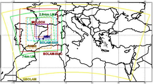
Fig. 2. Extension domains for the selected limited area models. Domains cover from entire Mediterranean Basin to Catalonia region. Solid
yellow line: QBOLAM. Solid green line: 7-km LM. Solid red line: BOLAM from ISAC-CNR. Dashed sky-blue line: BOLAM from SAR. Dashed orange line: RAMS. Dashed green line: 2.8-km LM. Dash-dotted blue line: MM5. Dash-dotted red line: MOLOCH.
– the Lokal Modell (LM) from Agenzia Regionale
Prevenzione e Ambiente of Emilia-Romagna region-Servizio Idro Meteo (ARPA-SIM).
Models are non-hydrostatic, excepted BOLAM and QBO-LAM, with horizontal grid size ranging from 2 km to 10 km, and domain size covering from Catalonia to the Mediter-ranean Basin (Fig. 2). The models also differ for the parame-terization schemes employed, and about initial and boundary conditions. In the operational configuration, these are pro-vided by ECMWF analysis and forecast for all models, ex-cept LM (DWD data) and MM5 (NCEP data).
However, for the Hydroptimet case studies, LM and MM5 simulations have been also performed using ECMWF data as initial and boundary conditions. Most of the models are ini-tialized with the 00:00 UTC ECMWF analysis of day 9 June, and take boundary conditions from the ECMWF forecast ini-tialized with the same analysis. The ISAC model chain dif-fers, since boundary conditions are taken from the ECMWF forecast started from the 12:00 UTC analysis of day 8 June. These are also the boundary conditions for QBOLAM run, but in this case the lower-resolution run is started 12 h in ad-vance, using 12:00 UTC ECMWF analysis of day 8 June as initial condition (cf. Table 1).
For each model only one run, starting from 00:00 UTC, 9 June 2000, is included in the intercomparison. Forecast range is 36 h, except QBOLAM whose forecast range is 48 h. Nevertheless, for the intercomparison study only the first 36 h of the QBOLAM simulation are considered here.
3.1.1 BOLAM-ISAC and MOLOCH
BOLAM, used for scientific purposes at ISAC-CNR, is a primitive equation, sigma-coordinate, hydrostatic model, with wind components, potential temperature, specific hu-midity and surface pressure as dependent variables.
Vari-ables are distributed on a non-uniformly spaced Lorenz grid. The horizontal discretization uses geographical coordinates, with latitudinal rotation on an Arakawa C-grid. Time integra-tion is based on a split-explicit integraintegra-tion scheme (Malguzzi and Tartaglione, 1999). This model version implements a Forward-Backward (FB) time integration scheme (Mesinger, 1977) for the term describing gravity waves and a Weighted Average Flux (WAF) scheme for the three-dimensional ad-vection. A detailed description of the dynamics and numeri-cal schemes can be found in Buzzi and Foschini (2000).
The water cycle for stratiform precipitation is described by means of five prognostic variables (cloud ice, cloud wa-ter, rain, snow, graupel), with a simplified approach similar to that proposed by Schultz (1995). Deep convection is parame-terized using the Kain-Fritsch (1990) convective scheme with some modifications, including those suggested by Spencer and Stensrud (1998) to improve the effect of the downdraft. The Ritter-Geleyn (1992) scheme is employed for parameter-ization of radiation. The orography used in the simulations is derived from interpolation and smoothing of the 1-km res-olution GLOBE Digital Elevation Model.
In the 36-h coarse-resolution Spanish run (160×160 grid points with spacing of 0.2◦in rotated coordinates and 38
vertical levels) the initial condition is supplied from the ECMWF analysis at 00:00 UTC, 9 June 2000, while bound-ary conditions are supplied from ECMWF forecasts from 12:00 UTC of the day before (12:00 UTC, 8 June 2000). Sequential self-nesting has been employed for the high-resolution experiment run, with grid spacing of 0.06◦(see Ta-ble 1).
MOLOCH is a non-hydrostatic high-resolution model that integrates the fully compressible set of equations with prog-nostic variables (pressure, temperature, humidity, horizontal and vertical velocity components) represented on the lat-lon rotated, Arakawa C-grid (Table 1). Hybrid terrain following
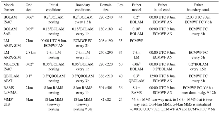
Table 1. Summary of models’ configuration for the Spanish case study. Each model is nested into a coarse-grid model referred as father
model. Father’s initial and boundary conditions are also included: unless it is differently specified, father’s boundary condition run starts from the analysis indicated under “Father’s initial conditions”. For each model simulation the forecast initial time is 00:00 UTC of 9 June 2000. Forecast range is 36 h for all models, except QBOLAM (48 h).
Model/ Grid Initial Boundary Domain Lev. Father Father Father Partner size conditions conditions size model initial cond. boundary cond. BOLAM 0.06◦ 0.2◦BOLAM 0.2◦BOLAM 220×240 44 0.2◦ 00:00 UTC 9 Jun. 12:00 UTC 8 Jun. ISAC nesting every 1.5 h BOLAM ECMWF AN ECMWF FC ∀ 6 h BOLAM 0.05◦ 0.18◦BOLAM 0.18◦BOLAM 180×180 42 0.18◦ 00:00 UTC 9 Jun. ECMWF FC SAR nesting every 1 h BOLAM ECMWF AN every 6 h LM 7 km 00:00 UTC 9 Jun. ECMWF FC 208×190 35 ECMWF
ARPA-SIM ECMWF AN every 3 h
LM 2.8 km 7-km LM 7-km LM 250×290 35 7-km 00:00 UTC 9 Jun. ECMWF FC ARPA-SIM nesting every 1 h LM ECMWF AN every 6 h MOLOCH 0.02◦ 0.06◦BOLAM 0.06◦BOLAM 220×220 50 0.06◦ 00:00 UTC 9 Jun. 0.2◦BOLAM ISAC nesting every 1 h BOLAM 0.2◦BOLAM every 1.5 h QBOLAM 0.1◦ 0.3◦QBOLAM 0.3◦QBOLAM 386×210 40 0.3◦ 12:00 UTC 8 Jun. ECMWF FC APAT nesting every 3 h QBOLAM ECMWF AN every 6 h RAMS 2 km 8-km RAMS 8-km RAMS 501×501 36 8-km 00:00 UTC 9 Jun. ECMWF FC, ∀ 6 h + LaMMA nesting every 1 h RAMS ECMWF AN inner-dom. nudg. ∀ 12 h MM5∗ 6 km 18-km MM5 18-km MM5 82×82 24 ∗6-km MM5 way nest. to 18-km MM5 that is two-UIB two-way two-way way nest. to 54-km MM5. 54-km MM5 is initialized
nesting nesting ∀ 3 h w. 00:00 UTC 9 Jun. ECMWF AN and ECMWF FC ∀ 6 h
coordinates, relaxing smoothly to horizontal surfaces away from the earth surface, are employed. Model dynamics is integrated in time with an implicit scheme for the verti-cal propagation of sound waves, while explicit, time-split schemes are implemented for the remaining terms. Three-dimensional advection is computed using the WAF scheme. Horizontal fourth order diffusion and divergence damping are included to prevent energy accumulation on the shorter space scales.
Some physical schemes (radiation, surface turbulent fluxes and vertical diffusion, soil water and energy balances) are provisionally similar to those of BOLAM, while the micro-physical scheme is new and partly based on the parameteri-zation proposed by Drofa (2003). The physical processes de-termining the time tendency of specific humidity, cloud wa-ter/ice and precipitating wawa-ter/ice are divided into “fast” and “slow” ones. Fast processes involve transformations between specific humidity and cloud quantities and are computed ev-ery advection time step. Fall of precipitation is computed, as a slow process, with the stable and dispersive backward-upstream scheme with fall velocities depending on concen-tration. Temperature is updated by imposing exact entropy conservation at constant pressure. The parameterization of the dry and moist convective adjustment is not considered, allowing the model to explicitly simulate atmospheric con-vection.
The model performance was evaluated by simulating some Mesoscale Alpine Programme (MAP) case stud-ies (Buzzi et al., 2004), characterized by heavy precipita-tion. MOLOCH is nested into the higher resolution BOLAM simulations, with lateral boundary values updated every hour (cf. Table 1).
3.1.2 BOLAM-SAR
Also for the Sardinia Meteorological Service (SAR), nu-merical simulation of the selected case studies have been carried out using a version of the limited area model BO-LAM, which is operationally used at SAR. As mentioned above, BOLAM is a primitive equation model resolved on a horizontal Arakawa C grid (rotated) and on vertical sigma levels (cf. Table 1). Time integration and parameteriza-tion schemes are the same as in BOLAM-ISAC, except for time integration of horizontal and vertical advection terms, which is accomplished with a Forward-Backward Advection Scheme (FBAS; Malguzzi and Tartaglione, 1999) instead of WAF.
For each case study two runs of the model are performed. The first run is obtained through a direct nesting of the 0.18◦BOLAM into the ECMWF global model. The second run is obtained nesting the 0.05◦BOLAM into the 0.18◦ BO-LAM using the aforementioned output as initial and bound-ary conditions. Moreover, two simulations have been done for the Spanish case changing the initial condition.
Firstly, in the 0.18◦ BOLAM the initial condition is
supplied from the ECMWF analysis at 12:00 UTC of 8 June 2000. Thus, for the 0.05◦BOLAM the initial
condi-tion is the 12 h BOLAM father forecast. Unfortunately, from this analysis the “Montserrat-2000” event was not forecast.
For the second experiment, the 0.18◦ BOLAM the ini-tial condition is supplied from the ECMWF analysis at 00:00 UTC of 9 June 2000 and the initial condition for the 0.05◦BOLAM is now the 0.18◦BOLAM father analysis (cf.
Table 1). From this analysis the “Montserrat-2000” event was forecast, but underestimated. This simulation is the one included in the intercomparison.
3.1.3 Lokal Modell
LM, the LAM of the Consortium for Small-scale Modelling (COSMO), is the meteorological model used by ARPA-SIM. LM, originally developed at the DWD (Offenbach, Ger-many), is based on the primitive hydro-thermodynamical equations describing compressible non-hydrostatic flow in a moist atmosphere without any scale approximations. The use of non-hydrostatic compressible (i.e. unfiltered) dynamical equations allows to avoid restrictions on the spatial scales and on the domain size. The equation of the vertical mo-ment is not approximate, so that it can describe much better those phenomena for which it is important to take into ac-count the vertical velocity (for example convective storms, sea and mountain breezes). The basic equations are written in advection form and the continuity equation is replaced by a prognostic equation for the perturbation pressure (i.e. the deviation of pressure from the reference state). The model equations are solved numerically using the traditional finite difference method.
The meteorological center of Emilia-Romagna, ARPA-SIM, has been using LM as the operational forecast model since 2001; LM is run twice a day (at 00:00 UTC and 12:00 UTC) for 72 h with a spatial horizontal resolution of 7 km and 35 levels in the vertical. The initial and boundary conditions for LM are obtained by interpolating respectively the values of the analysis and of the forecasts supplied by the global model of the DWD (one-way nesting). The boundary conditions are provided to the LAM every hour. Mesoscale data assimilation is also applied, using a nudging technique. LM simulations of the Hydroptimet case studies have been run in a slightly different configuration (cf. Table 1). The ini-tial conditions and the boundary conditions have been sup-plied by the global model of ECMWF. The model has been run at two horizontal resolutions, 7 and 2.8 km. The 7-km LM is nested on the ECMWF global model, while the 2.8-km version of LM is nested on the 7-2.8-km one. The initial and boundary conditions for the 2.8-km run are, then, provided by the 7-km run of LM. Both the 7-km and the 2.8-km LM simulations use the Tiedtke parametrisation scheme for cu-mulus convection.
3.1.4 MM5
MM5 model is running for research purposes at the UIB-Meteorological Group. Usually, the NCEP grid analyses, with a horizontal resolution of 2.5◦(in latitude-longitude coordinates), are employed at UIB to initialize the model and provide boundary conditions. The MM5 model grid is defined using the Lambert-Conformal Map Projection and therefore the NCEP analyses are interpolated on the MM5 grid.
Three mesoscale domains, interacting which each other, have been defined. For each domain, the origin of the coor-dinates is situated in the down-left corner of the grid. The grid size spacing is 54 km (domain 1), 18 km (domain 2) and 6 km (domain 3), each with 82 grid points both in lon-gitude and latitude direction and 24 vertical levels. The ratio between the size of one domain and its outer domain is 3:1, because a two-way interaction it has been applied. In fact, the 18-km MM5 is two-way nested to the 54-km MM5, and the 6-km MM5 is two-way nested to the 18-km MM5
The outer domain (domain 1) is centered in the northeast of Spain at geographical coordinate (39.0◦ N, 0.0◦ E) and measures 4374×4374 km. Domain 2 is approximately cen-tered over the Catalonia region, whereas the inner domain (domain 3) is approximately centered over Tarragona (see Fig. 2 for the 6-km domain extension).
For the control experiments, it has been used NCEP anal-ysis every 12 h (initial conditions and the rest of the time steps). The 54-km MM5 outputs are every 6 h, whilst for the other two domains outputs are every 3 h. Moreover, full physics is used and a Kain-Fritsch scheme is applied to pa-rameterize convection for the first domain, whereas no con-vective parameterization is present over the two inner do-mains.
Simulations using analysis and forecasts of the ECMWF have been also run, but results are not so good as those of the control experiment. This model configuration is used for the intercomparison study. The 54-km MM5 is initialized with ECMWF analysis at 00:00 UTC of 9 June 2000 and ECMWF forecast every 6 h as initial and boundary conditions, respec-tively (cf. Table 1).
3.1.5 QBOLAM
QBOLAM is a parallel version of the hydrostatic, primitive-equation, atmospheric limited area model BOLAM (Buzzi et al., 1994) implemented on a 128-processor QUADRICS APE-100 machine. It runs operationally at APAT in Rome, as a part of POSEIDON sea wave and tidal forecasting sys-tem (Speranza et al., 2004), which includes also a WAve Model (WAM), a Princeton Ocean Model (POM) nested on a Finite Element Model of the Venice Lagoon (VL-FEM) in cascade with the QBOLAM output.
Equations are discretized on a horizontal Arakawa-C grid, rotated in order to minimize grid anisotropy (Buzzi et al., 1998), and on a vertical sigma-level Lorenz (1960) scheme. As in BOLAM-SAR, the integration scheme employs FB to
describe gravity waves and FBAS for the horizontal and ver-tical advection terms. A fourth-order diffusion and a second-order divergence damping are also applied.
Due to massive parallelization issues, some parameteriza-tion schemes are simpler than in other BOLAM versions: they include analytic formulae (Louis et al., 1982), based on Monin-Obukhov similarity theory, to represent boundary-layer fluxes; a simplified radiation scheme (Page, 1986; Ruti et al., 1997); convection parameterization based on the Kuo (1974) scheme. A three-layer soil model provides lower boundary conditions.
For the case-study simulations, the operational configura-tion is used. The model is run on two one-way nested grids. The outer grid (162×98 points) has a horizontal spacing of 0.3◦in rotated coordinates, centered at the point of geograph-ical coordinate (38.5◦N, 12.5◦E), with an approximate ex-tension of 5300×3200 km, and 40 vertical sigma levels. Ini-tial conditions are provided by ECMWF analysis; boundary conditions are given by the ECMWF forecast initialized with the same analysis.
The inner domain (386×210 points) has a horizontal spac-ing of 0.1◦with an approximate extension of 4300×2300 km
(the other parameters are the same as above). The opera-tional, 60-h run starts daily with the 12:00 UTC analysis; however, the inner domain run starts 12 h later (spinup time) so that the higher resolution run has a 48-h forecast range, starting from 00:00 UTC of the day after the analysis. This run design was preserved in the case-study experiments. 3.1.6 RAMS
The RAMS model, operating at LaMMA since 1999 (Pasqui et al., 2000) integrates standard non-hydrostatic Reynolds-averaged primitive equations, compressible and time-split on a horizontal rotated (polar-stereographic transformation) and a vertical terrain-following coordinate. The physical pack-age of the model describes an atmospheric turbulent diffu-sion processes according with the Mellor-Yamada scheme, a cloud microphysics parameterization, a modified Kain-Fritsch type cumulus parameterization, the Harrington radia-tive transfer parameterization short and long wave scheme and the Land Ecosystem Atmosphere Feedback (LEAF) scheme for soil-vegetation-atmosphere energy and moisture exchanges.
The cloud microphysics scheme (Walko et al., 1995; Mey-ers et al., 1997) is a bulk microphysics representation of each hydrometeor category. This physics-based scheme empha-sizes individual microphysical processes rather than the sta-tistical end result of atmospheric systems; it is suitable to be applied to any kind of cloud (convective, stratiform, trop-ical etc.). The surface model (LEAF; Walko et al., 2000) evaluates fluxes of energy, water vapor, and momentum be-tween atmosphere and surface solving heat and water bal-ance equations for multiple soil layers, multiple snow cover layers, vegetation, and canopy air. LEAF uses a mosaic ap-proach to subdivide each surface grid cell into multiple land use types or “patches”. The LEAF model includes the effects
of freezing and melting, the temporary water and snow cover, the vegetation and the canopy air. The precipitation produced by both convective parameterization and bulk microphysical scheme, within the column grid, falls down on the vegetation coverage, producing a moisture fluxes and energy due to the different hydrometeors.
The simulation design is based on a two nested grids con-figuration at 8 and 2 km of grid spacing, respectively. Six-hourly ECMWF global model analysis fields provide both initial and boundary conditions on the outer grid, using both a lateral nudging, on a strong 6 h time scale, and a inner-domain light nudging on a 12 h time scale. This sort of “spec-tral nudging technique” is aimed to force the model with an-alyzed fields and, at the same time, let it develop its own dynamics in the domain far from lateral boundaries. Then, outer grid forecast provides one-way forcing for the 2-km grid spacing inner domain. Boundary conditions are pro-vided every 1 h only with a lateral nudging.
Over both grids, 36 vertical levels are present, with a stretched resolution from 50 m, near the surface, to 1100 m (cf. Table 1). In order to provide a better description of air-sea fluxes, observed weekly air-sea surface temperature fields at 9 km of resolution from AVHRR (NOAA) have been used. Initial soil temperature and moisture are set accordingly to available observed data for the interest period. A special precipitation microphysical scheme setting, originally devel-oped in the Hydroptimet framework, has been used: as one of the most critical microphysics scheme parameters is the “cloud condensations nuclei” (CCN) concentration for each hydrometeor categories, a special set-up has been chosen ac-cording to the mean total dust load, over the area, described by the Aerosol Index from TOMS satellite. In details, we define over the interest area three different dust load con-centration, namely low, moderate and high, with respect to the TOMS AI observed values. These conditions are direct linked with the CCN concentration. For each reference dust load condition we provide “the best choice”, of microphys-ical parameter settings for the RAMS simulation, obtained through analyzed case studies simulations (see for details Pasqui et al., 2004). Because not only the CCN concentration has a direct impact on precipitation, a “best” shape size dis-tribution choice for each hydrometeors categories has been provided as well.
3.2 Observed and forecast datasets
The verification data set includes 5-min rain gauge observed precipitations over Catalonia, 30-min satellite data, and 1-h model forecast precipitation fields for 9–10 June 2000. For the intercomparison study, forecast and observed precipita-tions have been accumulated at 3, 6 and 12 h over the entire event period.
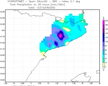
In Fig. 3 rain gauge observations accumulated on 36 h, starting from 00:00 UTC of 9 June 2000, are presented. The dense rain gauge network consists of 126 stations, covering an area of about 17 000 km2. Nevertheless, in order to have an observed rainfall analysis less sensitive to the grid box
Fig. 3. Precipitation observed by the Catalonia rain gauge
net-work during the “Montserrat-2000” event. Rainfall was accumu-lated from 00:00 UTC, 9 June to 12:00 UTC, 10 June 2000.
spacing selected for the intercomparison, a two-pass Barnes objective analysis scheme has been applied (Barnes, 1964, 1973; Koch et al., 1983). This procedure assigns a gaussian weight to each observation as a function of the distance be-tween rain gauge location and grid box center. The first pass produces a first guess gridded analysis, whereas the second pass increases the amount of detail from the previous one.
Further extension of the data set includes satellite rain-fall estimates interpolated on a grid with an equal spacing of 0.2 degrees for both coordinates (cf. Fig. 4). These estimates have been provided by LaMMA laboratory, which has im-plemented an operational chain that produces real-time half-hourly instantaneous rainfall maps. The procedure, operating in an autonomous, operational mode, is based on a blended technique (Turk et al., 2000a,b) that dynamically correlates brightness temperatures as measured by geostationary sen-sors and instantaneous precipitation levels, as computed by MW passive radiometer data (Ferraro and Marks, 1995; Fer-raro, 1997), by means of a statistical correlation (Crosson et al., 1996). The continuous streaming of geostationary and MW satellite data has been realized from ingesting ME-TEOSAT data from the local receiving system in one case, and downloading SSM/I data from an archive with near real-time data (i.e., SAA archive) in the other case.
The retrieved rainfall pattern (Fig. 4) does not show a good agreement with the rain gauge observations; in partic-ular, slight or no precipitation is estimated over the Llobre-gat basin, where the sharp rainfall peak, which produced the heaviest damages, is observed (Fig. 3). Actually, a weak rain band is present in Fig. 4, but with a strong south-easterly shift.
An error in the satellite estimate field can arise from a cal-ibration error or a time shift error in the retrieval algorithm; whereas a large-scale error in the rain gauge measurements is quite unlikely. For this reason, it has been decided to not
Fig. 4. 36-h satellite rainfall estimate, from 00:00 UTC, 9 June to
12:00 UTC, 10 June 2000.
use the satellite rainfall estimate for quantitative model veri-fication.
Another possible observational data source is the weather radar, located near Barcelona, of the Catalan Meteorological Service. Suitable algorithms for quantitative rainfall estima-tion have been developed (Rigo and Llasat, 2004), but their calibration needs further work and it is out of the scope of the present paper.
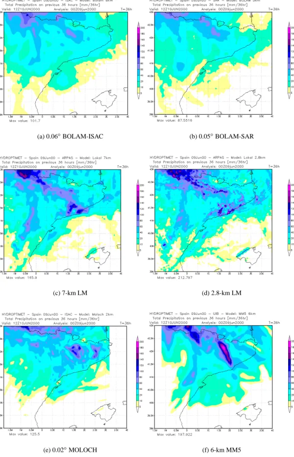
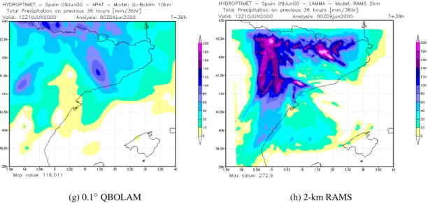
In Fig. 5 36-h precipitation forecasts predicted by the se-lected models over their own native grids are presented.
Since the models differ in the horizontal grid size, the in-tercomparison results may be sensitive to these differences. In fact, statistical intercomparison tends to be highly sensi-tive to forecast displacement error, especially when verify-ing on high-resolution grids or on a short accumulation time. Moreover, large errors are also expected when using a sin-gle rain gauge measure as a proxy of the average precipita-tion amount over an even very small area (Cherubini et al., 2002). Having more rain gauges per grid point is the most ef-fective way to deal with representation error, and this is done performing the statistical validation over a relatively coarse grid (Mass et al., 2002). Hence, model runs have been ver-ified on a common 10-km grid by means of the remapping grid-to-grid transformation (Accadia et al., 2003; Baldwin, 2000).
Although both procedures may change in a statistical way skill score results (Accadia et al., 2003), remapping, used op-erationally by the NCEP-Environmental Modeling Center, is better than a simple bilinear interpolation (used, for example, by ECMWF). First of all, bilinear interpolation treats grid-point precipitation values as defined at grid-points, whilst remap-ping considers gridpoint values as grid-box values. Further-more, bilinear interpolation may not be desirable for precip-itation, because it results in smoothing of the precipitation field. In addition, at variance with remapping, bilinear inter-polation does not conserve, to a desired degree of accuracy, the total precipitation forecast over the native grid.
(a) 0.06◦BOLAM-ISAC (b) 0.05◦BOLAM-SAR
(c) 7-km LM (d) 2.8-km LM
(e) 0.02◦MOLOCH (f) 6-km MM5
Fig. 5. Precipitation forecast by the selected LAMs over their own native grids. Rainfall was accumulated from 00:00 UTC, 9 June to
(g) 0.1◦QBOLAM (h) 2-km RAMS
Fig. 5. Continued.
4 Statistical and deterministic methodologies
To give a quantitative assessment about model skill in predicting the event, a statistical verification by means of widely-used non-parametric skill scores has been per-formed (Wilks, 1995; Schaefer, 1990; Hanssen and Kuipers, 1965; Mason, 1989).
These scores are tallied up on 2×2 contingency tables (Ta-ble 2), which summarize in a categorical way possi(Ta-ble com-binations of forecast and observed events above or below a given precipitation threshold. Hence, for each selected threshold, four categories are defined: hits; false alarms; misses and correct non-rain forecasts (see a, b, c and d in Table 2, respectively). The sum of these four category ele-ments, which is constant for each threshold, gives the sam-ple size, that is the total number of forecast/observation pairs over the verification period.
In order to have skill scores less sensitive to small change into contingency table population, they have been calculated on a sum of contingency tables (Hamill, 1999). In this case, since only one event is considered (36 h), the number of ta-bles depends on the accumulation time. For example, on a 12-h accumulation basis, categorical scores are tallied up on three contingency tables.
The BIA score, or bias score, (Wilks, 1995) is the ratio between the frequency of yes forecast and the frequency of yes observed. It is defined by:
BIA =a + b
a + c. (1)
A BIA equal to one means that the forecast is unbiased, that is forecasts and observations are above a selected threshold the same number of times. A BIA value greater than one in-dicates that the considered model overestimate the frequency of the events above a threshold (overforecasting); whereas a
Table 2. Contingency table of possible events for a selected
thresh-old. Rain observed Yes No Yes a b Rain forecast No c d
BIA value less than one indicates that the model underesti-mate the frequency of the events (underforecasting).
The equitable threat score (ETS; Schaefer, 1990) is an ac-curacy measure for binary forecasts. It is a modified version of the well-known critical success index (CSI; Wilks, 1995) that takes into account, as correction, the random forecast. In fact, the ETS score is defined by:
ETS = a − ar
a + b + c − ar
, (2)
where aris the number of model hits expected from a random
forecast:
ar=
(a + b) (a + c)
a + b + c + d . (3)
An ETS score equal to one indicates a perfect forecast; whereas a value close to 0 or negative means that the model has a questionable forecasting ability.
Another useful skill score is the Hanssen and Kuipers score (HK; Hanssen and Kuipers, 1965):
HK = (ad − bc)
(a + c) (b + d). (4)
Unlike the ETS score, this skill score gives a measures of the accuracy both for events and nonevents (McBride and Ebert,
2000). Moreover, it is independent of the event and nonevent marginal distribution. The score ranges between −1 to 1. A value equal to 1 means a perfect forecast, whilst a random forecast has a HK score close to zero. The HK score is equal to −1 when the number of hits and correct non-rain forecasts are both zero.
The false alarm ratio (FAR; Mason, 1989) is the ratio be-tween the number of false alarms and the total number of yes rain forecasts. Thus, the FAR is tallied up as:
FAR = b
a + b. (5)
As the FAR score is negative oriented, a model forecast with a FAR value close to zero is preferred (i.e., b = 0). Instead a FAR score equal to 1 means that all rain forecasts are false alarms (i.e., a = 0).
The thresholds set, depending on the accumulation time interval of forecasts and observations, includes high values, up to 80.0 mm/12 h, due to the high intensity of the observed space/time rainfall peak.
Once skill score verification results are available, it could be desirable to interpret them, going back to possible factors implied in score differences. Common techniques to deal with this nontrivial task are subjective analysis and sensitiv-ity studies.
However, a more straightforward approach, based on pat-tern analysis of contingency table elements, is here pre-sented. This approach might help to characterize the model error (e.g., with respect to orography, climatology etc.) and eventually to give hints about the error sources and the worth and shortcomings of the different model runs. Contingency table elements, used to compute the aforementioned skill scores, are utilized to identify for each simulation the ge-ographical zones in Catalonia where hits, misses and false alarms are concentrated. In fact, table elements are plot-ted, as a function of grid points, over the verification do-main showing the spatial distribution of hits, misses and false alarms.
Furthermore, to verify the spatial pattern matching of ob-served and forecast precipitations and to provide more in-sight on the forecast error sources (displacement, volume and pattern), the contiguous rain area analysis (CRA; Ebert and McBride, 2000) has been used. This object-oriented tech-nique is simply based on a pattern matching of two contigu-ous areas, defined as the observed and forecast precipitation areas, respectively, delimited by a chosen isohyet (or CRA rain rate contour).
When dealing with precipitation or, more in general, when the question is about forecast ability in matching the field maxima, the most suitable criterion to measure the spatial er-ror is the mean square erer-ror (MSE) minimization. Moreover, following this approach it is possible to decompose the error into three component sources: the displacement, the pattern and the volume errors.
The CRA analysis is performed shifting the gridded fore-cast precipitation field in latitude and longitude. However, to eliminate those matches that are not statistically significant at
the 95% confidence level, a minimum correlation value be-tween forecast and observation fields need to be achieved. This value is calculated following the approach presented by Xie and Arkin (1995) as a function of the number of ef-fective independent comparing grid points.
The CRA methodology gives also a quantitative support to the standard “eyeball” verification of model forecasts against rain gauge observations and satellite rainfall estimates.
For hydrological purposes, a quantitative deterministic verification obtained comparing observations and forecasts over Catalonia hydrological basins has been also performed. First of all, each verification grid point has been associated to the pertaining Catalonia basin (see Fig. 1). Then, precip-itations from each model simulation and rain gauge analysis have been accumulated over each basin for the 36-h period. Emphasizing the major impact areas, this analysis is quite useful in a hydrological perspective, provided the different extension of the basins is kept in mind (larger basins are less sensitive to spatial error).
5 Results and discussion
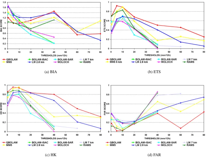
For brevity, only BIA, ETS, HK and FAR values for the 12-h accumulation time are discussed below, since values for shorter accumulation times substantially provide the same in-formation about the skill of the model runs.
The two LM versions, MM5 and QBOLAM display the same BIA trend (Fig. 6(a)): they overestimate the frequency of very light and medium-high intensity (40 mm/12 h) rain-fall, whilst they underestimate the occurrence of very strong rainfall. A similar trend, but closer to unity, is displayed by RAMS (Fig. 6(a)). The BIA scores for the two BOLAMs and MOLOCH display overestimation at low thresholds and un-derestimation at medium ones; whereas strong maxima are not predicted in the verification area (Fig. 6(a)). This state-ment is also true for the RAMS simulation. It looks like these model runs predicted diffuse precipitation in the verification area, instead of the sharp maxima shown by the observations. For this particular case, QBOLAM ETS scores (Fig. 6(b)) are better than those of associated to the other considered simulations. This is somewhat unexpected, since it is a hy-drostatic model with a relatively simple convection param-eterization and 10-km horizontal grid size. Also the high-resolution LM, MM5, and RAMS display a good skill, but not for all thresholds (RAMS only at the lowest thresholds; cf. Fig. 6(b)). Finally, the other four model runs (the two BO-LAMs, MOLOCH and the low-resolution LM) display a less performing behavior (Fig. 6(b)), suggesting that these sim-ulations did not match the observed high-intensity rainfall peak.
The HK results (Fig. 6(c)) have the same trend showed by the corresponding ETS results. Note that, in general, the HK values are higher than the corresponding ETS values, since the HK formula takes into account also correct non-rain fore-casts (cf. § 4).
(a) BIA (b) ETS
(c) HK (d) FAR
Fig. 6. 12-h BIA, ETS, HK and FAR calculated for the selected models remapped on a 10-km common grid. For graphical clarity, skill score
values less or equal to zero are not plotted.
For each model, FAR shows a general descending trend for the two lowest thresholds (Fig. 6(d)), indicating a small number of false alarms with respect of the yes forecasts. This trend is followed by an expected ascending trend (see previ-ously results), which means an increasing of the number of false alarms (Fig. 6(d)).
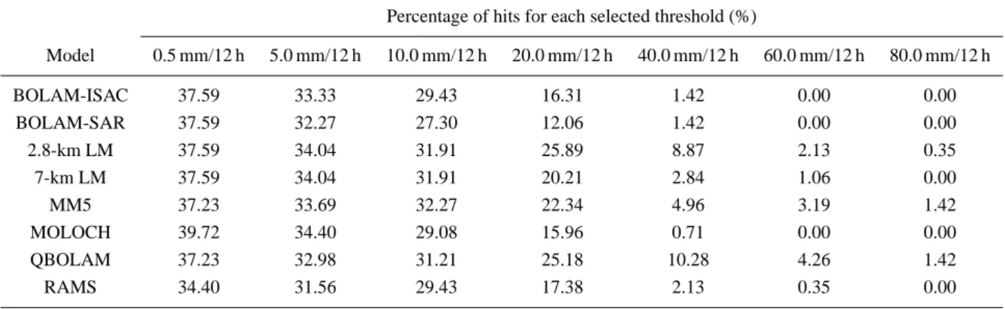
Moreover, to have an idea of the number of grid points where both observation and forecast are above the selected thresholds for the 12-h accumulation time, the percentage of hits, with respect to the sample size (282 pairs during the 36-h event), is presented in Table 3.
Graphical verification by means of the contingency table elements provides insight on the score differences discussed above (see Fig. 7 for misses spatial distribution).
The most skillful simulations (QBOLAM, 2.8-km LM) provide hits over all the event area, evidencing the most in-tense flood zone. MM5, 7-km LM and MOLOCH catch the widespread rainfall, but fail in capturing the precipita-tion peak. Only few hits are forecast by the other model runs (not shown). All models display misses on the peak zone (Montserrat), since they underestimate the magnitude of the
event (Fig. 7). The two BOLAMs display few false alarms and diffused misses (more simply, their forecast is too dry). Comparing patterns of false alarms and misses, shift errors can be detected, especially in MOLOCH and in the two LMs’ forecasts (not shown).
Quantitative verification can be also performed from a de-terministic point of view directly comparing observed and forecast rainfall amounts.
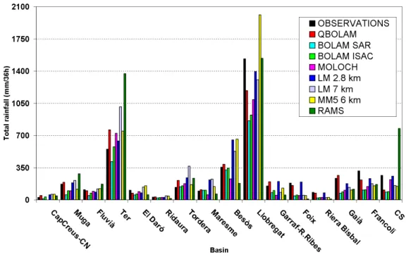
In Fig. 8 observed and predicted rainfall, accumulated for all the event time (36 h), are compared by basin. These val-ues outline a picture which partially differ from the one given by the skill score verification: for example, on the Llobregat basin RAMS prediction is quite good, whereas MM5 overes-timates the most intense peak. Such different evaluations of the skill are due, among other things, to the high sensitivity of the non-parametric skill score approach to small localiza-tion errors (double penalty effect). These results emphasize the multi-dimensional nature of the verification task: its re-sults are strongly dependent on the chosen forecast evalua-tion method, and eventually on the final forecast use.
(a) (b) (c)
(d) (e) (f)
(g) (h)
Fig. 7. An example of the spatial information given by a contingency table element verification approach. Misses were calculated on 3
h-based contingency tables for a 10.0 mm/3 h threshold. Each red cross indicates a grid point with at least one miss. If more than one miss is present during the 36-h simulation, it is indicated accordingly.
Table 3. Percentage of hits calculated on the 12-h accumulation time contingency tables. For each model simulation, values are catalogued
with respect to thresholds.
Percentage of hits for each selected threshold (%)
Model 0.5 mm/12 h 5.0 mm/12 h 10.0 mm/12 h 20.0 mm/12 h 40.0 mm/12 h 60.0 mm/12 h 80.0 mm/12 h BOLAM-ISAC 37.59 33.33 29.43 16.31 1.42 0.00 0.00 BOLAM-SAR 37.59 32.27 27.30 12.06 1.42 0.00 0.00 2.8-km LM 37.59 34.04 31.91 25.89 8.87 2.13 0.35 7-km LM 37.59 34.04 31.91 20.21 2.84 1.06 0.00 MM5 37.23 33.69 32.27 22.34 4.96 3.19 1.42 MOLOCH 39.72 34.40 29.08 15.96 0.71 0.00 0.00 QBOLAM 37.23 32.98 31.21 25.18 10.28 4.26 1.42 RAMS 34.40 31.56 29.43 17.38 2.13 0.35 0.00
Keeping in mind the description given in § 2, some insight on the forecast quality, and the representation of the relevant physical processes, is given by the comparison among ob-served and predicted precipitation patterns, both on a 36-h
accumulation base (cf. Figs. 3 and 5), and over shorter accumulation time intervals (not shown).
Actually, the observed squall line is not present in the two BOLAMs (Figs. 5(a) and 5(b)) and RAMS (Fig. 5(h))
Fig. 8. Total accumulated precipitation (from 00:00 UTC, 9 June to 12:00 UTC, 10 June 2000) over the inner Catalonia basins, from rain
gauge observations and models’ forecast.
forecasts, whereas rain is predicted to the north (on the Pyrenees) and to the west of the flooded area; it is also under-estimated in the BOLAMs’ forecast. MOLOCH (Fig. 5(e)), nested to BOLAM-ISAC, detects a strong rainfall peak, but with a sensible northward shift. The runs from the other four models tend to develop small scale structures similar to the observed squall line, which differ in shape and location. QBOLAM (Fig. 5(g)) and MM5 (Fig. 5(f)) forecast an elon-gated, compact band, located nearby the observed peak. The two LMs (Figs. 5(c) and 5(d)) show small, intense structures: the 7-km run reproduces the main peak, with a slight east-ward shift, while the 2.8-km run well reproduces the south-western and coastal secondary maxima.
A comparison over a 1-h accumulation period (not shown) evidences a strong match between the observed evolution of rainfall spatial distribution (a north-westerly elongated squall line moving eastwards) and the QBOLAM simulation; while the MM5 predicted precipitation starts north of the observed maximum location, then moving towards it. These results match, and in some sense explain, what has been seen in the discussion about the skill scores.
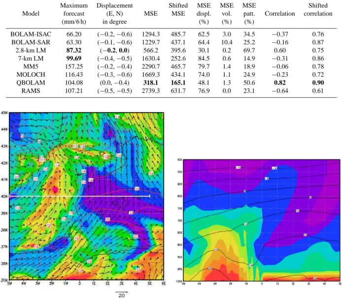
Such a qualitative discussion can be dealt in a more ob-jective way by means of CRA analysis. For the 6-h period of maximum observed rainfall intensity (from 00:00 UTC to 06:00 UTC of 10 June 2000), results are shown in Table 4.
On a 6-h basis, the error from two BOLAMs, MOLOCH, MM5, RAMS and especially from 7-km LM is mainly due to displacement component. For RAMS, MOLOCH, and the two BOLAMs the displacement to be applied to the forecast field to best fit the observed field is about 60–70 km (south-westwards).
This could be possibly due to a CRA matching of the observed peak with the much larger rainfall amount pre-dicted nearby the Pyrenees and not with the weak precipi-tation predicted on the flood zone. This problem may arise when verification is performed over a small domain, espe-cially when different rainfall forecast patterns are close in the area (Tartaglione et al., 2005). However after the CRA matching, for each simulation, not only the MSE decreases, but correlation strongly increases.
QBOLAM displays the smallest MSE (also after the CRA matching), almost all due to both pattern and displacement errors, whilst volume errors are small. On the contrary, the 2.8-km LM displays the smallest error shift, and most of the error is due to the pattern error source.
The CRA analysis has been also performed on the entire event (not shown). In many cases the 36-h results strongly differ from the 6-h ones, this could indicate the presence of a shift error variable in time. It is expected that a shift constant in time is associated mainly to large-scale dynamics forecast error, whereas a variable shift is more likely associated with errors due to representation of mesoscale processes.
All the aforementioned results provide a description of dif-ferent models’ precipitation forecast. Further work would be needed in order to try to explain different model per-formances in terms of model properties and run design via the representation of key atmospheric phenomena. A correct identification of such factors requires at least extensive sensi-tivity tests over all the involved models, and this lies outside the scopes of this work. However, a preliminary inspection of the predicted fields can provide some insight. In the fol-lowing some results are presented: first of all, the simulation from QBOLAM run (the one obtaining the highest scores, as
Table 4. CRA verification for 6 h (from 00:00 UTC to 06:00 UTC of 10 June 2000) intense rainfall of the Montserrat case study. A CRA rain
rate contour equal to 0.5 mm/6 h has been chosen. Maximum observed analysis equal to 95.16 mm/6 h. For each quantity, the best values are indicated in bold.
Maximum Displacement Shifted MSE MSE MSE Shifted Model forecast (E, N) MSE MSE displ. vol. patt. Correlation correlation
(mm/6 h) in degree (%) (%) (%) BOLAM-ISAC 66.20 (−0.2, −0.6) 1294.3 485.7 62.5 3.0 34.5 −0.37 0.76 BOLAM-SAR 63.30 (−0.1, −0.6) 1229.7 437.1 64.4 10.4 25.2 −0.16 0.87 2.8-km LM 87.32 (−0.2, 0.0) 566.2 395.6 30.1 0.2 69.7 0.60 0.75 7-km LM 99.69 (−0.4, −0.5) 1630.4 252.6 84.5 0.6 14.9 −0.31 0.86 MM5 157.25 (−0.2, −0.4) 2290.7 465.7 79.7 1.4 18.9 −0.06 0.78 MOLOCH 116.43 (−0.3, −0.6) 1669.3 434.1 74.0 1.1 24.9 −0.23 0.72 QBOLAM 104.08 (0.0, −0.4) 318.1 165.1 48.1 1.3 50.6 0.82 0.90 RAMS 107.21 (−0.5, −0.5) 2739.3 631.7 76.9 0.0 23.1 −0.64 0.61
Fig. 9. QBOLAM simulation verifying 12:00 UTC, 10 June 2000. (a) 850-hPa specific humidity (in color), temperature (red curves) and
wind (vectors) fields. (b) cross-section of specific humidity (in color) and temperature (black curves) along the white line indicated in (a).
in Fig. 6) is discussed in some detail; then a briefly subjective comparison with other two simulations (from BOLAM-SAR and MM5) is presented.
The 850-hPa QBOLAM forecast, few hours before the event (Fig. 5), evidences the key physical factor which in-fluence the rainfall distribution. Three air masses are con-verging on Catalonia: cold air is advected northerly from the Atlantic; moist, cyclonic air is present over the Iberian Penin-sula; warm air from the Western Mediterranean Sea is ad-vected southerly and forced eastwards by the Pyrenees. The different vertical structure of the last two air masses is evi-dent in the cross section in Fig. 5: deep convection is present over the land; a potentially unstable profile, with moisture
concentrated in the lower layers, over the sea. The conver-gence of these two air masses results in a “wet pool” over Catalonia, bounded northerly by the Pyrenees and westerly by the incoming cold Atlantic air. The mesoscale dynamics inside such a “pool” is responsible of the space-time rainfall distribution during the event.
Moreover, as an example, the 850-hPa fields over Cat-alonia forecast at 00:00 UTC of 10 June 2000 from QBO-LAM, the 6-km MM5 and BOLAM-SAR are compared. In Fig. 10 the main elements which affect the precipitation pro-cess are clearly visible: the distribution of the incoming air masses, the humidity pattern, the wind convergence zones, and the geopotential field structure. Such structures display
remarkable differences from model to model. This is not sur-prising, since a very different forecast skill among the three simulations was found (see, for example, Fig. 6).
However, the linkage between skill differences and pattern differences is far from evident. For example, QBOLAM pat-terns display more qualitative resemblance with ones from BOLAM-SAR (which has a lower skill) than with ones from MM5 (which has about the same skill); actually, much less moisture is present in the BOLAM-SAR run than in the other two.
It is possible that the different initialization between BOLAM-SAR and QBOLAM was responsible of such a dif-ferent moisture content, but it should be noted that BOLAM-SAR produces an even less skilled forecast when initialized as QBOLAM (see § 3.1.2).
Furthermore, wind convergence patterns are sharper in MM5 and BOLAM-SAR runs than in QBOLAM. This could be due to differences in resolution or in the parameterization schemes; however, it is not clear how this can affect the fore-cast quality. The westerly cold air spreads more eastward in MM5 than in QBOLAM; this can be reasonably related with the aforementioned north-eastward shift of MM5 predicted precipitation maximum.
At any rate, it is a quite nontrivial task to trace such mesoscale details back to the differences in model formula-tion, experimental design and initialization. Hence, this issue will require further work to be addressed.
6 Conclusions
The “Montserrat-2000” event is characterized by an excep-tional concentration of rainfall both in space and time: this makes a satisfying hydro-meteorological forecasting quite a challenging tasks for LAMs. The pros and cons of high-resolution, non-hydrostatic dynamics, or advanced cumulus parameterization schemes are not straightforward.
The verification study, performed with different statistical and deterministic, objective and subjective techniques, dis-plays a complex image of the different simulations’ perfor-mance. Results evidence a better forecast quality of QBO-LAM, MM5, and LMs simulations, essentially due to the development of a squall line over southern-central Catalo-nia, which is not caught by the other models. Furthermore, the forecast skill is affected by errors in position, orientation, texture and timing of the rain band, which vary among simu-lations.
An assessment of the effect of different model run ini-tializations should be preliminary to any interpretation of these results, especially considering that the highest skill scores are obtained by a run (QBOLAM) using a differ-ent initial analysis than the others. Anyway, at a first look, most of the models that show a better performance are non-hydrostatic, higher-resolution ones (LM, MM5). This indi-cates that high resolution is a valuable ingredient of fore-cast quality in this case, considering also that a large-scale shift error cannot be corrected only by enhancing the model
(a) QBOLAM
(b) 6-km MM5
(c) BOLAM-SAR
Fig. 10. 850-hPa forecast over Catalonia of specific humidity (in color), geopotential height (black curves) and wind verifying 00:00 UTC, 10 June 2000.
resolution. However, this assessment is not fully unambigu-ous. In fact, the QBOLAM simulation shows the best perfor-mance despite its lower resolution, hydrostaticity and simple parameterization schemes. Since the main QBOLAM advan-tage is its large domain extension, this may suggest a signif-icant role of the domain extension in shaping a correct fore-cast of this case study.
An essential factor in this sense could be the correct rep-resentation of meso-synoptic forcing patterns, which shape the circulation over Catalonia by the convergence of three air masses coming from western Mediterranean, Iberian Penin-sula and Atlantic Ocean and the barrier effect of the Pyre-nees. How these factors operate in the single simulations, and how this depends on model properties and configura-tions, run initialization, etc., will be the object of future stud-ies.
Acknowledgements. The authors thank Hydroptimet partners who
made forecast and observed data available to us. We thank also Giuseppina Monacelli (APAT), Tomeu Rigo (Univ. of Barcelona), Tiziana Paccagnella and Chiara Marsigli (ARPA-SIM), Andrea Buzzi (ISAC-CNR), Piero Chessa (SAR), Massimiliano Pasqui and Samantha Melani (LaMMA) and Alberto Mart´ın Garc´ıa (Univ. of Illes Balears). Comments and suggestions received during the workshops were very useful.
Edited by: A. Buzzi Reviewed by: two referees
References
Accadia, C., Mariani, S., Casaioli, M., Lavagnini, A., and Speranza, A.: Sensitivity of precipitation forecast skill scores to bilinear interpolation and a simple nearest-neighbor average method on high-resolution verification grids, Weather Forecast., 23, 453– 469, 2003.
Baldwin, M.: Quantitative Precipitation Forecast Verification Doc-umentation, Tech. rep., NCEP/EMC, www.emc.ncep.noaa.gov/ mmb/ylin/pcpverif/scores/docs/mbdoc/pptmethod.html, 2000. Barnes, S. L.: A technique for maximizing details in numerical
weather map analysis, J. Appl. Meteorol., 3, 396–409, 1964. Barnes, S. L.: Mesoscale objective analysis using weighted
time-series observations, NOAA, National Severe Storm Laboratory, Norman, OK 73069, tech. memo. ERL NSSL-62, 1973. Buzzi, A. and Foschini, L.: Mesoscale meteorological features
as-sociated with heavy precipitation in the southern Alpine region, Meteorol. Atmos. Phys., 72, 131–146, 2000.
Buzzi, A., Fantini, M., Malguzzi, P., and Nerozzi, F.: Validation of a limited area model in cases of Mediterranean cyclogenesis: surface fields and precipitation scores, Meteorol. Atmos. Phys., 53, 53–67, 1994.
Buzzi, A., Tartaglione, N., and Malguzzi, P.: Numerical Simula-tion of the 1994 Piedmont Flood: Role of Orography and moist processes, Mon. Weather Rev., 126, 2369–2383, 1998.
Buzzi, A., Davolio, S., D’Isidoro, M., and Malguzzi, P.: The im-pact of resolution and of 4-D Var reanalysis on the simulations of heavy precipitation in MAP cases, Meteor. Z., 13, 91–97, 2004. Cherubini, T., Ghelli, A., and Lalaurette, F.: Verification of
pre-cipitation forecasts over the Alpine region using a high-density observing network, Weather Forecast., 17, 238–249, 2002.
Crosson, W. L., Duchon, C. E., Raghavan, R., and Goodman, S. J.: Assessment of rainfall estimates using a standard Z-R relation-ship and the probability matching method applied to composite radar data in central Florida, J. Appl. Meteorol., 35, 1203–1219, 1996.
Drofa, O. V.: The parameterization of microphysical processes for atmospheric numerical models, Nuovo Cimento, 26C, 233–262, 2003.
Ebert, E. E. and McBride, J. L.: Verification of precipitation in weather systems: determination of systematic errors, J. Hydrol., 239, 179–202, 2000.
Ferraro, R. R.: Special sensor microwave imager derived global rainfall estimates for climatological applications, J. Geophys. Res., 102(D14), 16 715–16 735, 1997.
Ferraro, R. R. and Marks, G. F.: The development of SSM/I rain-rate retrieval algorithms using ground-based radar measure-ments, J. Atmos. Ocean. Technol., 12, 755–770, 1995.
Hamill, T. M.: Hypothesis tests for evaluating numerical precipita-tion forecasts, Weather Forecast., 14, 155–167, 1999.
Hanssen, A. W. and Kuipers, W. J. A.: On the relationship be-tween the frequency of rain and various meteorological parame-ters, Meded. Verh., 81, 2–15, 1965.
Kain, J. S. and Fritsch, J. M.: A one-dimensional entrain-ing/detraining plume model and its application in convective pa-rameterization, J. Atmos. Sci., 47, 2784–2802, 1990.
Koch, S. E., desJardins, M., and Kocin, P. J.: An interactive Barnes objective map analysis scheme for use with satellite and conven-tional data, J. Climate Appl. Meteor., 22, 1487–1503, 1983. Kuo, H. L.: Further studies of the parameterization of the influence
of cumulus convection on large scale flow, J. Atmos. Sci., 31, 1232–1240, 1974.
Llasat, C., Barriendos, M., and Rigo, T.: The “Montserrat-2000” flash-flood event: a comparison with the floods that have oc-curred in the northeast Iberian Peninsula since the 14th century, Int. J. Climatol., 23, 453–469, 2003.
Lorenz, E. N.: Energy and numerical weather prediction, Tellus, 12, 364–373, 1960.
Louis, J. F., Tiedtke, M., and Geleyn, J. F.: A short history of the PBL parameterization at ECMWF, proceedings of the ECMWF workshop on planetary boundary layer parameteriza-tion, ECMWF, 25–27 November 1982, Reading, UK, 1982. Malguzzi, P. and Tartaglione, N.: An economical second order
ad-vection scheme for numerical weather prediction, Quart. J. Roy. Meteorol. Soc., 125, 2291–2303, 1999.
Mason, I.: Dependence of the critical success index on sample cli-mate and threshold probability, Aust. Meteorol. Mag., 37, 75–81, 1989.
Mass, C. F., Ovens, D., Westrick, K., and Colle, B. A.: Does Increasing Horizontal Resolution Produce More Skillful Fore-casts?, Bull. Amer. Meteorol. Soc., 83, 407–430, 2002. McBride, J. L. and Ebert, E. E.: Verification of quantitative
precip-itation forecasts from operational numerical weather prediction models over Australia, Weather Forecast., 15, 103–121, 2000. Mesinger, F.: Forward-backward scheme and its use in a LAM,
At-mos. Phys., 50, 200–210, 1977.
Meyers, M. P., Walko, R. L., Harrington, J., and Cotton, W. R.: New RAMS cloud microphysics parameterization. Part II: The two-moment scheme, Atmos. Res., 45, 3–39, 1997.
Page, J. K.: Prediction of solar radiation on inclined surfaces, D. Reidel Publishing Company, Dordrecht, 1986.
Pasqui, M., Gozzini, B., Grifoni, D., Meneguzzo, F., Messeri, G., Pieri, M., Rossi, M., and Zipoli, G.: Performances of the opera-tional RAMS in a Mediterranean region as regards to quantitative precipitation forecasts. Sensitivity of precipitation and wind fore-casts to the representation of the land cover, proceedings of the 4th RAMS Users Workshop, Cook College-Rutgers University, 22–24 May 2000, New Jersey, USA, 2000.
Pasqui, M., Pasi, F., and Gozzini, B.: Sahara dust impact on precip-itation in severe storm events over west-central Mediterranean area, Proceedings of the 14th International Conference on Cloud and Precipitation, 18–23 July 2004, Bologna, Italy, 1, 181–184, 2004.
Rigo, T. and Llasat, M. C.: A methodology for the classification of convective structures using meteorological radar: Application to heavy rainfall events on the Mediterranean coast of the Iberian Peninsula, Nat. Hazards Earth Syst. Sci., 4, 59–68, 2004,
SRef-ID: 1684-9981/nhess/2004-4-59.
Ritter, B. and Geleyn, J. F.: A comprehensive radiation scheme for numerical weather prediction models with potential applications in climate simulations, Mon. Weather Rev., 120, 303–325, 1992. Ruti, P. M., Cassardo, C., Cacciamani, C., Paccagnella, T., Longhetto, A., and Bargagli, A.: Intercomparison between BATS and LSPM surface schemes, using point micrometeorological data set, Beitr. Phys. Atmos., 70, 201–220, 1997.
Schaefer, J. T.: The critical success index as an indicator of warning skill, Weather Forecast., 5, 570–575, 1990.
Schultz, P.: An explicit cloud physics parameterization for oper-ational numerical weather prediction, Mon. Weather Rev., 123, 3331–3343, 1995.
Spencer, P. L. and Stensrud, D. J.: Simulating flash flood events: importance of the subgrid representation of the convection, Mon. Weather Rev., 126, 2284–2912, 1998.
Speranza, A., Accadia, C., Casaioli, M., Mariani, S., Monacelli, G., Inghilesi, R., Tartaglione, N., Ruti, P. M., Carillo, A., Bargagli, A., Pisacane, G., Valentinotti, F., and Lavagnini, A.: POSEI-DON: an integrated system for analysis and forecast of hydro-logical, meteorological and surface marine fields in the Mediter-ranean area, Nuovo Cimento, 27, 329–345, 2004.
Tartaglione, N., Mariani, S., Accadia, C., Speranza, A., and Ca-saioli, M.: Comparison of raingauge observation with modeled precipitation over Cyprus using contiguous rain area analysis, Atmos. Chem. Phys. Discuss., 5, 2355–2376, 2005.
Turk, F. J., Hawkins, J., Smith, E. A., Marzano, F. S., Mugnai, A., and Levizzani, V.: Combining SSM/I, TRMM and infrared geo-stationary satellite data in a near-realtime fashion for rapid pre-cipitation updates: advantages and limitations, pp. 452–459, Pro-ceedings of the 2000 EUMETSAT Meteorological Satellite Data Users’ Conference, 2000a.
Turk, J. F., Rohaly, G., Hawkins, J., Smith, E. A., Marzano, F. S., Mugnai, A., and Levizzani, V.: Meteorological applications of precipitation estimation from combined SSM/I, TRMM and geo-stationary satellite data, VSP Int. Sci. Publisher, Utrecht (The Netherlands), 2000b.
Walko, R. L., Cotton, W. R., Meyers, M. P., and Harrington, J.: New RAMS cloud microphysics parameterization. Part I: The single-moment scheme, Atmos. Res., 38, 29–62, 1995.
Walko, R. L., Band, L. E., Baron, J., Kittel, T. G. F., Lammers, R., Lee, T. J., Ojima, D., Pielke, R. A., Taylor, C., Tague, C., Trem-back, C. J., and Vidale, P. L.: Coupled atmosphere-biophysics-hydrology models for environmental modeling, J. Appl. Meteo-rol., 39, 931–944, 2000.
Wilks, D. S.: Statistical methods in the atmospheric sciences: an introduction, Academic Press, San Diego (USA), 1995. Xie, P. and Arkin, P. A.: An intercomparison of gauge observations
and satellite estimates of monthly precipitation, J. Appl. Meteo-rol., 34, 1143–1160, 1995.