M
Maassssaacchhuusseettttss IInnssttiittuuttee ooff T
Teecchhnnoollooggyy
E
Ennggiinneeeerriinngg SSyysstteem
mss D
Diivviissiioonn
Working Paper Series
ESD-WP-2006-19
B
ULK
P
OWER
G
RID
R
ISK
A
NALYSIS
:
R
ANKING
I
NFRASTRUCTURE
E
LEMENTS
A
CCORDING TO THEIR
R
ISK
S
IGNIFICANCE
A. M. Koonce
1, G. E. Apostolakis
2, and B. K. Cook
31Massachusetts Institute of Technology
Department of Nuclear Science and Engineering
2Massachusetts Institute of Technology
Department of Nuclear Science and Engineering Engineering Systems Division apostola@mit.edu
3Sandia National Laboratories
Albuquerque, New Mexico
Bulk Power Grid Risk Analysis: Ranking Infrastructure
Elements According to their Risk Significance
A. M. Koonce
1, G. E. Apostolakis
1,*, and B. K. Cook
21Department of Nuclear Science and Engineering,
Massachusetts Institute of Technology, Cambridge, MA 02139-4307, USA
2Sandia National Laboratories, Albuquerque, NM 87185-0671, USA
Abstract
Disruptions in the bulk power grid can result in very diverse consequences that include economic, social, physical, and psychological impacts. In addition, power
outages do not affect all end-users of the system in the same manner. For these reasons, a risk analysis of bulk power systems requires more than determining the likelihood and magnitude of power outages; it must also include the diverse impacts power outages have on the users of the system.
We propose a methodology for performing a risk analysis on the bulk power system. A power flow simulation model is used to determine the likelihood and extent of power outages when components within the system fail to perform their designed
function. The consequences associated with these failures are determined by looking at the type and number of customers affected. Stakeholder input is used to evaluate the relative importance of these consequences. The methodology culminates with a ranking of each system component by its risk significance to the stakeholders. The analysis is performed for failures of infrastructure elements due to both random causes and malevolent acts.
Key Words: bulk power grid; risk analysis; random failures; terrorism
1. Introduction
The electric supply system in North America including the United States, Canada, and a small portion of Northern Baja, Mexico, can be viewed as consisting of three parts: the generation of electric power, the transmission of electricity, and the distribution of electricity to the end-users. The bulk power system is the generation and transmission portion of the system. The term ‘bulk’ refers to the large amounts of electric power carried by the system before it is distributed to the end-users [1].
The bulk power grid is an international system that is divided into three major regions. These regions are collectively known as the NERC (North American Electric Reliability Council) Interconnections and include the Eastern Interconnection, the Western Interconnection, and the ERCOT (Electric Reliability Council of Texas) Interconnection. The Eastern Interconnection services the U.S. states and Canadian provinces east of, and including, the Great Plains region. The Western Interconnection provides power to states and provinces west of, and including, the Rocky Mountain area. The smallest interconnection, ERCOT Interconnection, covers the majority of Texas. These interconnections exhibit strong connectivity within themselves but are only weakly connected to each other.
Electric power supports almost every aspect of our daily lives, either directly or indirectly, and has become an integral part of our national security and economy. A diverse set of end-user groups constitute the customers of the bulk power. These users include individual citizens, manufacturers, financial networks, communication
companies, transportation networks, medical facilities, government agencies, and gas and water supply infrastructures. The bulk power grid forms the transportation backbone through which power flows from generation facilities to the distribution networks that
ultimately supply power to most end-users†.
In light of recent events, such as the 2003 Northeast Blackout, and the prevalent dependencies on electric power, it is recognized that a large disruption in the bulk power system, either due to random events or intentional attacks, may result in widespread consequences. These consequences could include economic, social, physical, and psychological impacts. The blackout of the Northeast on August 14, 2003 affected over 50 million people and has been estimated to have had an economic impact between $4 billion and $10 billion in the United States alone [2].
There is a large amount of literature that analyzes failures in the bulk power system as they impact the economy. Zimmerman et al. [3] have developed a
methodology that employs the economic accounting concept. The methodology uses cost factors to assign a monetary value to the consequences (loss of life, business losses, and loss of services) that may result from terrorist attacks on the bulk power system. The authors then combine these dollar values into a single measure, the economic impact, which is used to evaluate the risk terrorist attacks pose to the power grid. Greenburg [4] illustrates the use of this methodology by developing a terrorist attack scenario on the New Jersey electric power supply network and evaluates the impacts on the New Jersey economy. The economic impacts of the August 14, 2003 Northeast Blackout as stated in [2] were also based on economic evaluations of metrics that included spoilage of
perishable goods, cost of power not provided, lost productivity, disposal of goods in
production during power outage, extra wages for employees, and equipment restart expenses. As stated earlier, there are various types of impacts (social, physical, and psychological) that accompany economic impacts with failures in the bulk power grid, some of which may be socially unacceptable to be assigned a dollar ‘cost.’
Analysis of past blackout data [5] show that outages and disturbances follow a power law distribution with a tail that shows that larger blackout frequencies decrease as a power function of its size. This is contrary to the previous belief that the frequencies of major blackouts decreased exponentially. Chen et al [6] confirm this distribution, and its tail, by analyzing NERC data of power outages that date back to 1984. Carreras et al [7] further investigate this distribution of blackout sizes by looking for critical loading points in electric power systems. They present an electric power transmission model that represents loads and generators as nodes of a network and use linear programming to analyze the network. Load shedding is observed as the load demand of the system is increased and the capacity of supply is held constant. This study shows that there are two transitions that define a critical loading that greatly increases the risk of major blackouts. One transition occurs when the load demand overcomes the total capacity of generation. A second transition occurs when load demand causes the transmission lines to become overloaded. Criticality of electric transmission systems was verified by Nedic et al. [8] using AC power modeling.
There are also studies that look at ‘hardening’ effects of the bulk power grid against terrorist attacks. Salmeron et al. [9] use non-linear programming to construct a power flow model that establishes the load flow of an electric power grid system. Lines are then attacked, or removed from service, and the power flow model is used to
reestablish a stable configuration with portions of the system’s load not served. The effects on the system are tracked as multiple lines are removed from service. These results are used to find the optimal applications of available resources to harden the system and minimize the effects of terrorist action. Bier et al [10] introduce a linear programming algorithm that also solves this optimization problem of applying available resources to the power grid with similar results as the previous work.
Engineers at the Duke Power Company have proposed a value-based approach to investment planning regarding upgrades to the power system [11]. Their methodology looks at the expected cost of proposed improvements and the expected cost to customers of future outages without this improvement. They combine the customer cost and investment cost to determine the minimal value over a time period using discounting of future costs. The lowest value of the combined cost determines the appropriate time to make the improvement to the transmission system. To do this, the engineers look at the likelihood of future outages, the possible effects of these outages, and the cost imposed onto the customers if these outages occur. This work looks at the direct economic impact to customers that result from power outages but not the social, physical, and
psychological impacts.
This paper focuses on analyzing the risks associated with the bulk power system using the viewpoint of an electric utility company. Section 2 summarizes our past work on risk assessment which is the basis for the methodology developed and applied to the bulk power grid in Section 3. Section 4 offers a discussion of the results and, finally, Section 5 offers several concluding remarks.
2. Risk Assessment
2.1 Overview
There are three components that make up risk in a technological system. These are the sequences of failures that can lead to undesirable consequences, their likelihood of occurrence, and the consequences that accompany these failures. This triplet definition of risk was proposed by Kaplan and Garrick [12] when they defined risk as the answers to the following three questions:
• What can happen? • How likely is it to occur? • What are the consequences?
There are methods, such as Probabilistic Risk Assessment (PRA; also called Quantitative Risk Assessment - QRA), for answering these three questions in complex but well defined systems such as nuclear power stations, chemical processing plants, and space systems [13]. For large, national infrastructures, these methods need to be adapted to the infrastructure’s technological and sociopolitical complexities [14]. Garrick et al [15] outline a possible application of PRA techniques in the analysis of infrastructures. They point out that the full application of these techniques requires the development of processes by which private and government bodies will be able to share data freely. The difficulty in applying these methods to the risk assessment of infrastructures is further exacerbated when terrorism or malevolent acts are to be considered due to problems with determining the likelihood of a successful attack. The assessment of the likelihood that a terrorist attack will occur requires information on the intent, capability, and resources to carry out the attack. Given that a group possesses these traits, determining the point, or points, of attack requires knowledge of the goals, beliefs, and desires of the group. The probability of the attack being successful depends upon the quality of countermeasures in place to deter or combat the attack [16]. For these reasons, the MIT methodology (to be described shortly) assumes threats of appropriate levels for the analysis and leaves the likelihood of attack to the agencies responsible for collecting intelligence [14]. The risk assessment of infrastructures presents additional difficulties due to their diffuse nature.
To answer the first two risk questions when dealing with infrastructures, the ideas of vulnerabilities and threats are used. Haimes [17] defines these two terms as follows:
“Vulnerability is the manifestation of the inherent states of the system (e.g. physical, technical, organizational, cultural) that can be exploited to adversely affect (cause harm or damage to) that system.”
“Threat is the intent and capability to adversely affect (cause harm or damage to) the system by adversely changing its states.”
We adopt these definitions in this paper.
2.2 The MIT Methodology
Apostolakis and Lemon [14] develop a screening methodology for diffuse
infrastructures and rank vulnerabilities to terrorism. The authors apply their methodology to the water, electric power, and gas distribution systems on the Massachusetts Institute of Technology (MIT) campus. The methodology requires the stakeholders to determine the importance of possible consequences that may result from successful attacks on these infrastructures. These consequences include impacts on public image, Institute
operations, economics, health, safety, and the environment. Thus, in addressing the first PRA question (what can happen?), these authors go beyond the usual consequences that are related to health, safety, and economics. The stakeholder group in this work is a multidisciplinary team that includes decision makers of the MIT Department of Facilities with expertise in finance, utility operations, and space planning [18].
The stakeholder input is used to create a value tree that reflects the stakeholder views. A minimal cut set (mcs) approach is used to identify and analyze vulnerabilities in the infrastructures. The consequences resulting from successful attack on the
vulnerabilities are then applied to the value tree to determine the stakeholder impact (value) each vulnerability represents. Apostolakis and Lemon point out that determining the likelihood of a terrorist attack is very difficult and is best left to the security and intelligence agencies. Their work assumes a “minor” level of threat to be present. The work then determines the susceptibility of each mcs to this level of threat by looking at its accessibility and security measures. The susceptibility of each mcs is then combined with its value for ranking. The result is a ranking that requires a mcs to have both a high susceptibility and a high value to be placed higher in the ranking.
Michaud and Apostolakis [19] expand this methodology by analyzing a water supply network for an entire city. The authors use network theory and component capacity to analyze the water supply infrastructure rather than the mcs approached employed in Reference 14. Michaud and Apostolakis also expand the methodology by including the duration of system failures in their analysis to capture the time dependence of the consequences resulting from failures in the infrastructure. These authors do not look only at terrorist acts on the infrastructure but split the threats to the system into mechanical (random) failures and malevolent acts. This allows the analysis to rank the infrastructure elements according to their impact on the stakeholders when these elements fail randomly and when they are disabled by malevolent acts.
Patterson and Apostolakis [20] further develop the MIT ranking methodology by identifying critical locations within multiple infrastructures. Critical locations are those where an attack will affect more than one infrastructure. The authors apply the
methodology to the chilled water supply, domestic water supply, steam supply, natural gas, and electric power infrastructures on the MIT campus. The Geographic Information System (GIS) is employed to determine the geographical layout of each infrastructure. GIS also provides extensive data on the infrastructure user groups identified within the work. Due to the larger number of infrastructures and users included in the analysis, the authors use Monte Carlo simulation and importance measure concepts for the analysis of each infrastructure. The authors borrow the concept of importance measures from PRA [21- 22] and they generalize it to include the stakeholder values. Each infrastructure is analyzed independently to assign to each location a value of the new importance measure the authors call Geographic Valued Worth (GVW). Once each infrastructure is analyzed, the GVWs from each infrastructure for a given location are summed to determine the location’s overall GVW. These GVWs are used to rank the various locations.
The next section describes the MIT methodology, as it applies to the bulk power grid, in detail. Details of the grid and customer groups used in the work are also
3. Methodology
3.1 Overview
The MIT risk ranking methodology is a systematic process to analyze failures in an infrastructure and rank them according to their impacts on the stakeholders. The work presented in this paper is the result of collaboration between MIT and Sandia National Laboratories to apply the methodology developed in [14, 19, and 20] to the bulk power grid. The stakeholders used in this presentation are five members of an electric utility company. Figure 1 illustrates the methodology. Although details will be provided later, a brief overview is given here.
The methodology begins by identifying assets and components of the bulk power infrastructure that will be included in the analysis. Analysis of the infrastructure is then performed using the Sandia AC load flow simulation model [23] to determine the physical consequences resulting from the failure of the components. The consequences include the number and type of customers affected, and the duration of the power
outages. These consequences are input to a value tree that incorporates the stakeholders’ views of possible impacts. The value tree is then used to determine the impact the consequences have on these stakeholders. The amount of impact a component represents to the stakeholder is its value. Each component value is then combined with its
susceptibility to failure or attack. The combination of value and susceptibility is then used to rank the components according to their risk significance. The following subsections describe the process of this methodology in detail.
3.2 Infrastructure Elements
The IEEE 1996 Reliability Test System (RTS-96) [24] is a test grid that has been established to evaluate bulk power reliability analysis techniques. The system does not resemble any portion of the North American power grid but has been developed to provide a universal standard that could be used for diverse applications [24]. The single area RTS-96 is used as the study grid for our application.
The single area RTS-96 grid (Figure 2) contains 24 buses and 38 transmission lines. The buses consist of 9 load only buses, 8 load/generation buses, 3 generation only buses, and 4 transmission buses (no load or generation on the bus). Reference [24] provides data for generators, buses, and transmission lines that include capacities, failure rates and probabilities, mean times to repair/failure (MTTR/MTTF), and line lengths. However, there are no established customers associated with the RTS-96 grid. This requires that an artificial customer set be created and placed on the grid for our work.
We introduce four customer groups: Residential customers, Commercial
customers, Small – Medium Industrial customers, and Large Industrial customers. These customer groups were selected based on Edison Electric Institute [25], which identifies the customer groups as Residential, Commercial, and Industrial. The Industrial customer group was split into two groups, small – medium and large, so that the differences
between these customer types could be included in the analysis, e.g., the impact due to down time, equipment re-start time, and the loss of product that results from power interruptions as discussed in the IEEE Gold Book [26].
Customers for each customer group were placed on each load bus using national average usage data [25] and the load history for the system [26]. These customers were added to each group until the load capacity of the RTS-96 was reached. Table 1 shows the customer loading. To simulate diversity within the grid, the customers are not placed in the same ratio among the groups on each bus. These customer groups were developed and applied to the grid prior to the infrastructure analysis. For application to an actual portion of the North American power grid, an assessment of the customers on the grid would be required. This assessment could be done using the utility company’s customer data or by surveying the area which the analysis would cover.
The infrastructure elements whose failures will be investigated are the generators, buses, and transmission lines that make up the bulk power grid. The threats to these elements include both random failures and malevolent acts. Malevolent acts are the intentional disruption of the infrastructure by purposely preventing a component from carrying out its designed operation.
Single-failure scenarios are used as the failure scenarios in the presentation of this methodology. As for attacks, only minor threats are considered. Minor threats are threats, such as vandalism or employee sabotage, that have the ability to attack a single infrastructure asset, but do not possess the ability to attack multiple assets with a coordinated attack. Even though the failure of multiple components would likely have larger consequences, the likelihood of multiple failures may decrease significantly, a fact that would offset partly their importance or value in the ranking process. This single-component limitation was made in part due to the limitations of the model used to analyze the power grid at this time and due to the rapidly increasing number of
combinations of simultaneous events. If the present work included an actual portion of the North American power grid, the investigation of higher-order vulnerabilities would need to be covered to include coordinated attacks on multiple targets, as well as
concurrent failures of two or more assets.
3.3 Infrastructure Analysis
The infrastructure analysis of the bulk power grid employs an AC load flow simulation model developed at Sandia National Laboratories [24]. For input into the load flow model, the single area RTS-96 is modeled as a network that includes the buses as nodes and the transmission lines as arcs. Node data include the real and reactive power generating capacity, the real and reactive power load demand, the customer loading, and the peak load history for each day in a 52 week year (364 days). Arc data include the voltage and current capacities [24]. The load flow model is currently limited to modeling only one generator per bus. Work is underway to update the program’s generator
modeling characteristics and allow for the modeling of multiple generators on each bus. The analysis presented in this work combines the total generating capacity on each bus and treats it as a single generator.
Figure 3 provides an overview of the power systems analysis. Grid analysis begins by selecting a system component (generator, transmission line, or bus) to be failed and the time frame for the analysis. The analysis time frame can be any time length between one day and 364 days (the entire load history period). This allows the analysis of the bulk power grid to be performed using varying seasonal data, such as the effects of
the weather on component failure rates/frequencies and the consequences resulting from component failures during extreme cold/hot seasons. The number of days selected in the time frame will be the number of simulations run for the selected component.
Transmission Line 4 is selected as the failed component along with a time frame of 21 days and will serve as the example throughout this section.
The load flow model uses a series of steady-state AC simulations to estimate the effects that an initial, single-component failure has on the entire infrastructure. This multiple-step, quasi-transient approach has the ability to follow the progress failure of the system by identifying components in the grid that experience conditions outside of their limits, e.g., transmission lines that experience over-current conditions, and are then tripped off line. The model’s crude simulation of cascading failures can result in the initial, single-component failure causing more load shed than a normal stability analysis would conclude. This model is admittedly imperfect but was used here to facilitate the proof-of-concept application of the methodology.
The power flow model begins by initializing the system with a stable flow for the first day of the time frame. To do this, the system loading for the day is determined by the load history data provided in the RTS-96. The day’s peak load is assumed to last the entire day. A stable flow is established when the existing load is being supplied with power from available generators and each transmission line is within its voltage and current capacities.
Once the system is in a fault-free, stable condition, the selected component is failed (Transmission Line 4 for our example). The introduced fault of the selected component causes a disturbance in the power flow. The simulation model adjusts the generated power at each generator to attempt to regain a stable flow in response to this disturbance. Power is adjusted until the generating capacity is reached or the load is met on each bus, which ever occurs first. The current and voltage on each transmission line is tracked during this power adjustment.
Any transmission line that has a voltage below its limit requires load to be shed in order to bring the line voltage within specifications. Load shedding is done in 10% increments of the total bus load. This incremental load shed is done to simulate the segregation of load by the various branches leaving the bus in the distribution system. This simplifying assumption is made due to the RTS-96 not possessing an established distribution system that further carries the electric power from the bulk power grid to the end users. If an actual portion of the North American bulk power system were analyzed, where the distribution system is identifiable, the increments of load that may be shed at each bus would be determined by the configuration and priority of each branch in the distribution system. After each transmission line voltage is verified within its limits, the current on each line is investigated.
The simulation model identifies the transmission lines that are carrying a current above its limit. Transmission lines with excessive current will be tripped out of service and will require additional adjustment to the load flow. Any adjustment to the load flow will require the transmission line voltages to be reevaluated as in the previous step.
Once a stable load flow has been reestablished, the amount of load shed at each bus is recorded within a load shed vector and the simulation is repeated for the next day in the time frame or terminates if the time frame is complete. To complete the analysis of
the components in the system, the entire simulation process is repeated for each remaining component using the same time frame.
The load shed vector is an N-dimensional vector that represents the effect the failed component has on the system with N being the number of buses in the grid. N is 24 for the single area RTS-96 grid. Each element of the load shed vector is the
percentage of load at its respective bus that has been shed to regain stability in the
system. The elements that correspond to a transmission bus (no customers present on the bus) will always be zero. Since the simulation can encompass several days, a separate load shed vector is produced for each day of the simulation time frame. Our example time frame is 21 days; therefore, 21 load shed vectors are produced for the failure of transmission line 4.
The affected component, the number and type of customers affected, and the duration of the power outages make up the physical consequences of system failures. The type and number of customers affected by load shedding is determined by the load shed vectors. It is assumed for the RTS-96 customer base that the customers on a bus are evenly dispersed over the distribution system branches (10% increments) of the bus. That is, if a bus experiences a 20% load shedding during a failure scenario, 20% of each customer group on that bus will be shed to meet the load shedding requirement. The duration of the power outage is determined by the failed component. The duration of a failure scenario is assumed to be the component’s mean time to repair (MTTR) or permanent outage duration time as specified in the RTS-96. For our example,
Transmission Line 4 is the failed component so the duration of the scenario is 10 hours. This time equates to the required time to repair the line and is listed as its permanent outage duration time listed in [24].
As mentioned previously, the time frame selected for the analysis determines the number of load shed vectors calculated for each component in the system. Due to the system load history (a different peak load for each day), these load shed vectors for a single component may vary throughout the time frame. We assume that the load shed vector that results in the largest amount of load shed is the representative vector for the component. The customer portion of the physical consequences of losing Transmission Line 4 is given in Table 2. The zero elements of the load shed vector are omitted since there would be no load loss on their associated buses. Shedding a portion of a single customer is not allowed; for this reason, there are no large industrial customers lost upon failure of Transmission Line 4.
3.4 Value Tree and Constructed Scales
The value tree is based on multi-attribute utility theory (MAUT) and provides a hierarchical view of the impact each failure scenario may have on the stakeholders. The value tree consists of three levels in which the top level is the overall impact, or value, of a failure scenario (Figure 1). The second level breaks this overall impact into broad categories called impact categories (IC). The ICs are further reduced in the third level to specific aspects, called performance measures (PM), that specifically describe the various ways consequences result in impacts to the stakeholders. Each PM is divided into
various levels of impact called the constructed scales (CS). The levels of the CSs represent the amount of impact the physical consequences have on the stakeholder
through each PM. The levels for each CS range from no impact to complete impact to the PM.
The value tree is constructed using stakeholder input regarding the ways in which they may be affected by system failures. This is done by the stakeholders defining the ICs, PMs, and CS that make up their value tree. Once the value tree is formed, the stakeholders’ view of importance regarding each IC, PM, and CS is modeled. The importance modeling is done by assessing the stakeholders’ beliefs using pairwise comparisons. These comparisons are then used in calculating the weights for the ICs, PMs, and each level in the CSs. The IC and PM weights represent their contributions to the overall impact. The weight of a CS level represents the amount of impact felt by the stakeholders when the physical consequences result in that level. Since the impacts felt by the stakeholders are negative impacts, the amount of impact is referred to as the disutility.
For each failure scenario, the physical consequences result in a CS level being impacted for each PM. The PM weights and disutility is then used to determine the overall impact felt by the stakeholder. The overall impact of a scenario is called its performance index (PI) and is used in the component ranking process.
The construction of the value tree and its weights used for the present work are presented here as an example of this methodology. The CSs used in this work are then discussed followed by an example of the process used to determining the PI of each failure scenario.
The stakeholders who participated in the construction of the value tree are five members of a regional electric utility company affiliated with the management and transmission departments at the company, Table 3. They worked together to form the value tree in a workshop. Input for the weights associated with the value tree was provided independently by each member. The input provided by the senior participating member, referred to as S-1, will be the primary input for this work and is presented as the example in this section. The input provided by the remaining four members (S-2 through S-5) will be discussed in the next section and used as a sensitivity analysis on the
application of the methodology.
Figure 1 contains the value tree that represents the consensus of the five stakeholders (excluding the weights). Economics, Image, Health & Safety, and
Environment were defined as the ICs and were deemed sufficient to encompass all
possible impacts felt by the company following a failure in the power grid. Economics was divided into Lost Revenue, which accounts for the financial impacts due to power not supplied during an outage, and Repair/Replace, which is the cost associated with
restoring the failed component. Image defines the impacts to the company’s image following an outage and was split into the company’s Political, Public, and Customer image. Political defines the impact system failures have on the local, state, and federal authorities which may propose additional regulations on electric generating and
transmission companies. Public refers to the general public’s view of and confidence in the company’s ability to provide reliable power. Customer defines the company’s relationship with non-residential customers and is assumed to be directly tied to the customer’s incurred cost due to a power outage. Health & Safety was divided into
General Public and Utility Workers. General Public is meant to account for the effects
transportation networks, and daily life conveniences such as heating and cooling a home.
Utility Workers accounts for the increased safety concerns of the company regarding its
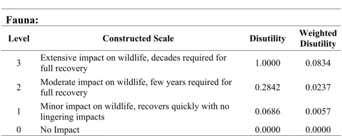
employees that are responsible for repairing the failed component. Environment was assigned a single PM which is Fauna. Fauna defines the effect failure scenarios have on the wildlife in the region with specific consideration to fish population linked to the operation of hydroelectric generators.
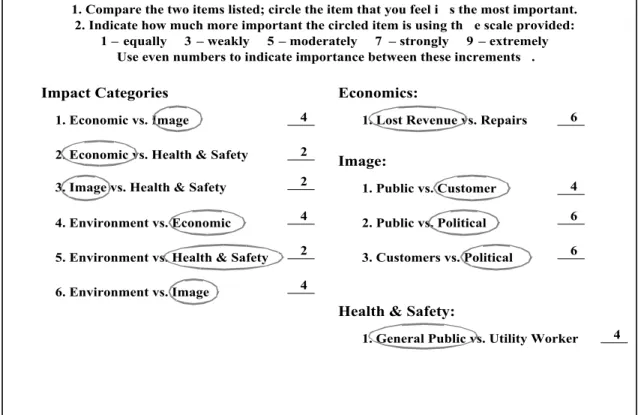
To evaluate the weights present in the value tree, the participating members were provided surveys in which they performed pairwise comparisons between the ICs. They first identified which ICs they felt were more important and to what extent. This process is shown in Figure 4 (using the input provided by S-1). For example, this stakeholder judges that the IC Health & Safety is equally or slightly more important than the IC
Environment. The same stakeholder believes that the PM General Public is weakly to
moderately more important than the PM Utility Workers with respect to Health & Safety. It is very important to point out that the stakeholders have already been informed about the possible ranges of the consequences and are making their evaluations being fully aware of these ranges. In the present case, it was the consensus that the potential impacts of failures on both Health & Safety and the Environment were very small, unless a major catastrophic event disrupted a majority of the grid. The stakeholder assessments were made under this assumption.
The stakeholder input is placed into a matrix and the weights are determined using the Analytic Hierarchy Process (AHP) [27]. Although several methods exist in the literature for evaluating weights [28], this method was used because the stakeholders find the pairwise comparisons easier to implement. The AHP results were scrutinized to make sure they represented the stakeholder views.
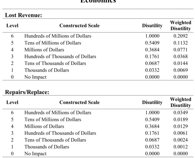
The CSs used for this work are presented in Table 4 – Table 7. AHP is also used for the determination of the disutility for each level of the CSs. Disutility is a
monotonically non-decreasing function that defines the amount of impact a level in the CS has on its PM. For this reason, the disutilities in each CS range from no impact (0.0000) to complete impact (1.0000) of the PM.
To determine the level in which physical consequences impact the stakeholders, the physical consequences are mapped onto the CSs of each PM. The mapping technique used is determined as shown in Table 8. Sum means that the effects on each customer group are determined and then summed to determine the level of impact. The
consequence matrix follows the approach presented in [19] where the effects on each customer group are determined and then the customer group that results in the highest level of impact is chosen as the representative group for the PM. Component specific means that the level of impact is determined solely by the failed component in the failure scenario. Inspection means that the effects a failure scenario has on the infrastructure itself and not the customers is used to determine the level of impact. An example of each mapping technique is presented here using our example failure scenario (Transmission Line 4, with a 21-day time frame) to help clarify the process.
Sum is only used by the Lost Revenue PM. Each customer group has an associated average energy consumption (kWh) and rate charged per unit of energy consumed ($/kWh). The physical consequences give us the number of customers in each group that is affected and the duration of the outage. Using this information we have:
( ) ( )
( )
[
N
R
U
]
( )
T
$
n 1 i i i i⋅
⋅
⋅
=
∑
= where;$ is the resulting lost revenue
n is the number of customer groups included in the analysis (four in our case)
Ni is the number of customers in group i
Ri is the rate charged to a customer in group i
i
U is the average electric power usage for a single customer in group i
T is the duration of the scenario
The lost revenue for our example is $140,525. This results in transmission line 4 being placed in level 3 for Lost Revenue which has a disutility of 0.1761 to the stakeholder (Table 4).
The mapping technique (Table 8) “Component Specific” will be illustrated using the Repair/Replace PM. The cost to restore a failed component depends on the
component itself and the way the component failed. The component may be able to be repaired or might be required to be replaced, depending on the level of damage to the component. The cost should include the price of repair parts as well as the cost of equipment used and wages paid due to the man-hours required to restore the component. Company historical data may also be used to evaluate the average cost to restore a type of component and to determine its impact. Here, we assume that the cost to restore a
transmission line does not exceed $50,000 but is no less than $10,000. This assumption is based on the required cost to repair a transmission line by looking at the labor of the worker, equipment operation cost, and material cost associated with the repairs. This puts Transmission Line 4 into level 2 for Repair/Replace which has a disutility of 0.0687 to the stakeholder.
The consequence matrix requires the construction of a matrix that relates the duration and number of customers affected by a failure scenario to the CS. This is done by evaluating the response of the customer groups to past power outages of various sizes and durations. We use discrete estimates of magnitude and duration of the physical consequences to determine the expected impact level for the CS. The consequence matrix for the Customer PM is provided in Table 9 for our example. The physical consequences for Transmission Line 4 (Table 2) lead to a level 3 impact based on Commercial, a level 3 based on S-M Industrial, and a level 0 based on Large Industrial. Since the maximum level among all groups is a level 3 impact, transmission line 4 is put into level 3 with a 0.3317 disutility to the stakeholder (Table 5).
The mapping technique “Inspection” is used only in the Fauna PM and is focused on the effects caused during power production increases at hydroelectric facilities that result in an impact on the local fish population. As power is increased at a hydroelectric generator, more water is forced through the generating house which results in less water that is allowed to bypass. Affecting this ratio of power production and bypass flow has effects on the fish population in the river. For this reason, the amount of power increase at these facilities and the duration of this power increase are the factors that affect this PM. Since the output of the simulation model (load shed vectors) did not directly give the increase in power production at each generation location, this information is
determined through inspection.
The difference between the amount of load shed and generation disconnected from the grid during a failure scenario is used to determine the increase demand placed on the generators remaining connected to the grid. It is also assumed that any increase in
demand will be shared among the remaining generators. This difference in the amount of generation disconnected and load shed is used to create a unique consequence matrix for this PM and is presented in Table 10. The values in this matrix represent the amount of excess load that will be placed onto the remaining generators, including the hydroelectric facilities. If a failure scenario results in more load shed than generation disconnected, or if the hydro plants are disconnected from the grid, the effect on the Fauna PM is
evaluated at a level 0. Transmission Line 4 results in a generation lost to load shed of -174 MW which results in a level 0 impact with a 0.0000 disutility to the stakeholder.
To determine the performance index (PI) of a failure scenario, we use Equation 2 [14]
∑
= = PM K 1 i i ij j wd PI wherePIj is the performance index of failure scenario j
wi is the weight of performance measure i
dij is the disutility of performance measure i and failure scenario j
KPM is the total number of performance measures
Table 11 gives an overview of the level of impact to each PM along with the PM weights for our example failure scenario (stakeholder S-1). Using the disutilities, PM weights for S-1, and equation 2, the resulting PI for Transmission Line 4 is 0.0884. This PI
represents the value the failure of Transmission Line 4 has to S-1.
3.5 Ranking
The work presented up to this point has been focused on determining the value of failure scenarios in the bulk power grid. So far, the first and third questions of risk assessment have been answered. The second question (likelihood) remains to be addressed.
To review before we continue, there were two types of threats addressed by this methodology, random events and minor malevolent acts. As discussed earlier, while the likelihood of random events is determined by the scenario frequency, the likelihood of malevolent acts is not addressed by this methodology but, rather, the susceptibility to an assumed threat is evaluated [19].
For random failures, the frequency of a failure scenario is multiplied by the scenario’s value to determine the expected disutility to the stakeholder. As described in [19], the random failures of the infrastructure elements are then ranked according to their expected disutility.
For malevolent acts, the “susceptibility” of a component is judged subjectively by accessing the quality of security measures and openness of the component. Reference [14] proposes six levels of susceptibility to malevolent acts ranging from completely secure (the lowest level) to completely open (the highest level). These susceptibility levels are given in Table 12.
As proposed in [14] each component’s PI and susceptibility are combined in order to assign the component to a vulnerability category. This process is illustrated in Table 13. The vulnerability categories are shown in Table 14.
The present work assesses transmission lines to have an extreme susceptibility (Level 5) due to their openness and remote locations. Buses are assessed to have moderate susceptibility (level 3) due to safety fences and possible video surveillance. Generators are usually located at facilities with security forces and high authorized personnel traffic. For this reason, generators are assessed to have a very low susceptibility (level 1).
To complete our example of the failure of Transmission Line 4, its random failure frequency is 0.39 failures/year. Multiplying this frequency with its PI, we calculate the expected performance index for this transmission line to be 0.03448.
The susceptibility category for transmission lines is extreme and Transmission Line 4 possesses a moderate PI, which results in the line being assigned to the Orange category for vulnerabilities (Table 14).
4. Discussion
4.1 Stakeholder S-1
The input provided by stakeholder S-1 is used to determine the baseline results for our analysis of the RTS-96 single area grid. S-1 valued Economics and Image as the most important impact categories and this resulted in the Lost Revenue, Political Image, and Customer Image performance measures being the dominant contributors to the overall value of each failure scenario. The top ten components ranked by their risk significance with respect to malevolent acts and random events are provided in Table 15 and Table 16, respectively.
An in-depth look at the results for the vulnerability rankings shows that there are two major reasons for T-16 and T-17 being placed at the top of the list. These
transmission lines connect the upper portion of the grid, where the majority of the generation is located, to the lower portion of the grid. When these lines fail, they limit the amount of power that can be transmitted to the lower portion of the grid causing the transmission lines in the lower portion of the grid to become stressed by increasing their loading. This increased loading results in Transmission Line T-5 becoming overloaded and tripping thus increasing the scenario’s impact on bus 6. This results in a large number of customers being shed. Transmission lines T-16 and T-17 also have extremely long power outage durations due to their long repair times. This combination of duration and magnitude causes a high-level impact to both Political Image and Lost Revenue.
Another interesting result of the vulnerability ranking for S-1 is that the amount of load shed alone does not determine the order in which the components are ranked. This observation is illustrated by the components ranked #6 through #10. The last two
components of the ranking, B-3 and B-4, result in very large load sheds. However, T-14, T-15, and T-13 are ranked higher even though they result in a smaller load shed. This is due to the transmission lines having a much longer outage time. The duration is the key factor here that elevates their impacts to stakeholder S-1. It should also be noted that the varying distribution of customer groups at affected load busses and the associated
variations in impacts also contribute to a nonlinear relationship between the load shed and the disutility of a failure scenario.
Looking at the results for the random failure events, high failure frequency was the dominant consideration for the rankings. Transmission line T-13, ranked #1, is one of two lines that connect a remote load bus, B-6, to the grid. Upon failure of T-13, only moderate load shed results due to the other line connected to B-6 having the ability to be loaded more and minimizing the impact. However, due to its relatively high failure frequency, T-13 represents the most expected disutility to stakeholder S-1 by resulting in moderate impact to Lost Revenue and Customer Image. The components that resulted in higher load shed usually were associated with very low failure frequencies which reduced their expected impacts to S-1.
It was expected that the value of each generator would be high given the
limitation placed on the modeling of generation at each bus. It was also expected that the buses would result in large consequences due to the load directly connected to the bus being completely lost when it fails. The infrastructure analysis did result in a large amount of load being shed when a bus or generator was selected as the initial failed component, which would have caused them to stand out in a conventional stability
analysis of the grid. However, transmission lines are the highest ranked contributors with respect to both random events (expected disutility) and malevolent acts (vulnerability) for stakeholder S-1. As discussed above, this is due to the fact that the amount of load shed is only one of the factors that determine risk significance. In general, the high
susceptibility level (extreme) and higher failure frequencies of the transmission lines are the key factors that elevate them in the rankings above the other types of components even though the amount of load shed is usually smaller.
4.2 Sensitivity Evaluation
To determine the sensitivity of the results to the input provided by the various participating members, the component rankings were produced using each stakeholder’s input. The rankings from each stakeholder are then compared to evaluate their
differences.
As shown in Table 17, the five stakeholders’ views of importance of the ICs include many differences. This provided very strong differences in the weights of each performance measure. The top ten components ranked by their vulnerability level and expected disutility for each stakeholder are presented in Table 18 and 19, respectively.
The results of the comparisons between the component rankings of the stakeholders are surprising. Each stakeholder’s vulnerability ranking results in very similar results with few differences in the components identified, the order of the components, and the vulnerability levels associated with each component within the rankings. Inspection of the effects each IC has on the overall value for each stakeholder resulted in the following findings:
• The Economics and Image ICs are more sensitive than the other ICs to the range of physical consequences that can result from component failures in the grid. • The Health & Safety and Environment ICs have very little influence on the overall
failure scenario impact unless the physical consequences include a lengthy duration and/or a very large number of customers are affected by the scenario.
Even though S-3, S-4, and S-5 rank Health & Safety and Environment highly, the higher level of these ICs are not affected until the physical consequences reach a very large scale. In order to impact these higher levels, almost half of the power grid would need to be shed which did not occurred in this study. This was in line with the consensus reached at the input elicitation workshop that the impact to Health & Safety and Environment was small unless a catastrophic event takes place. Without the higher scales of these IC being affected, the Economics and Image ICs are the key factors that determine a component’s value. This results in similar random event and malevolent act rankings of the
components among all stakeholders.
5. Concluding Remarks
The methodology presented in this paper provides a systematic process that produces a ranking of the elements within the bulk power grid for random failures and malevolent acts. This ranking is not solely determined by the amount of load shed when a specific component experiences failure. Rather, the multiple aspects that make up the risk a component failure poses to the system, as determined by the impacts to the stakeholders, are used to determine the ranking. The reasons for each component’s position in the rankings are identifiable and can be traced back to the stakeholder
preferences and the infrastructure itself. These results should be viewed as a first input to a deliberation by the stakeholders in which their reasonableness of the rankings is
debated and the assumptions of the analysis scrutinized [29]. The results of this analysis process are also stakeholder dependent. Any other stakeholder, such as a federal agency like the Department of Homeland Security, could include additional PMs and discard some that we have included in our study. However, the methodology is unchanged and would result in a component ranking appropriate for the new stakeholder’s views.
There are several areas in which additional work is required to improve the analysis. The identification and modeling of more specific customer groups would improve the value assessment of each component in the grid by allowing a more specific look at the effects on customers during power outages. Customer prioritization for load shedding would also increase the accuracy of the analysis by not including the customers that pay a premium for more reliable service in most load shedding scenarios.
Application of this methodology to an actual portion of the North American power grid would also provide the realism needed to generate more support for the methodology. The power flow simulation model is in its infancy and is being improved regarding its generator modeling capabilities and load shedding scheme. This will allow the results for forced outages of generators to be more realistic. Further improvements to the model will also include mitigation measures to minimize load shedding to better reflect the application of such in the industry. However, it should be noted that the methodology is model agnostic, and therefore a more sophisticated load flow model could be easily substituted in the future.
It is also realized that placing each component into a susceptibility level but its type is also not completely realistic, such as all buses in the Moderate susceptibility level. This assumption eliminates probably the most significant risk to a substation, the
intentional vandalism of transformers. To increase the accuracy of the analysis, the analyst must identify each component’s susceptibility on a case by cases basis. This was
not possible with the application of the RTS-96 single area grid due to the limited data provided for each component.
This paper’s purpose is to present the MIT risk ranking methodology as it applies to the bulk power grid. The load flow simulation model and the analysis of the RTS-96 test system used in the presentation of this methodology is not the focal point. Analysts of a real power grid are not bound to perform the infrastructure analysis in the manner described here and may choose any method of analysis suitable to meet their needs. The assumptions made in this paper are sometimes broad and may appear to oversimplify the analysis. By incorporating a more comprehensive assessment of the disutility of various failure scenarios, we do believe that the methodology presented here has advantages over the traditional contingency analysis performed today by many utilities and could
potentially provide the industry with a more consistent and meaningful way to identify critical assets, as may be required under the new NERC Critical Infrastructure Protection (CIP) standards. Future work will evaluate the application of this methodology to a real power system in collaboration with a utility partner.
Acknowledgments
We thank Bryan Richardson of Sandia National Laboratories for his help with the power flow simulation model used in this work. We also appreciate the helpful discussions with David Robinson of Sandia on general approaches to assessing risk in complex
infrastructure systems and the power grid in particular. We gratefully acknowledge support from Sandia’s Laboratory Directed Research and Development Program (LDRD). Sandia is a multiprogram laboratory operated by Sandia Corporation, a Lockheed Martin Company, for the United States Department of Energy’s National Nuclear Security Administration under contract DOE. No. DE-AC04-94AL85000.
Figure Captions
Figure 1: Methodology overview.
Figure 2: Single area IEEE RTS-96 grid (Ref. 24). Figure 3: Infrastructure analysis overview.
Infrastructure Elements
Analysis
Power Flow Modeling MTTF & MTTR
Physical Consequences
Element Ranking
Health and Safety (3) 0.1667 Economics (2) 0.2441 Image (1) 0.5058 General Public (8) 0.0333 Political (1) 0.3693 Lost Revenue (2) 0.2092 Repair / Replace (7) 0.0349
Overall Value to the Stakeholder Utility Workers (3) 0.1334 Customer (4) 0.0977 Public (6) 0.0388 Value Impact Categories Performance Measures Value Tree Environment (4) 0.0834 Fauna (5) 0.0834
Figure 3: Sandia Load Flow Model Analysis Overview [23]. Initialize system power flow Fail selected component Evaluate transmission line voltages Shed 10% of load at buses supplied by affected transmission line Voltage to low Adjust system power flow
Produce load shed vector All voltages within limits Evaluate transmission line currents Remove affected transmission lines from service Current above limit All currents within limits Another day in time frame? No Terminate simulation
(Load shed vectors are recorded)
Yes
Set system load to the next day load
Instructions:
1. Compare the two items listed; circle the item that you feel i s the most important. 2. Indicate how much more important the circled item is using th e scale provided:
1 – equally 3 – weakly 5 – moderately 7 – strongly 9 – extremely Use even numbers to indicate importance between these increments .
Impact Categories
1. Economic vs. Image
2. Economic vs. Health & Safety 3. Image vs. Health & Safety 4. Environment vs. Economic 5. Environment vs. Health & Safety 6. Environment vs. Image
Economics:
1. Lost Revenue vs. Repairs
Image:
1. Public vs. Customer 2. Public vs. Political 3. Customers vs. Political
Health & Safety:
1. General Public vs. Utility Worker 2 2 2 4 4 4 6 6 6 4 4
Table Captions
Table 1: Customer data per bus.
Table 2: Customer portion of physical consequences for transmission line 4. Table 3: Participating members’ affiliation with the electric utility company. Table 4: Constructed scales for Economics performance measures.
Table 5: Constructed scales for Image Performance Measures.
Table 6: Constructed scales for Health & Safety performance measures. Table 7: Constructed scales for Environment performance measures. Table 8: PM mapping techniques.
Table 9: Consequence matrix for Customer PM Table 10: Matrix for Fauna PM.
Table 11: Impacts to each PM for transmission line 4. Table 12: Susceptibility levels of infrastructure elements.
Table 13: Susceptibility and value combinations for each vulnerability category.
Table 14: Infrastructure asset vulnerability categories for ranking element failures due to malevolent acts.
Table 15: Top 10 components ranked by vulnerability level for S-1 (minor malevolent acts).
Table 16: Top 10 components ranked according to their expected disutility for S-1 (random failures).
Table 17: Value tree weights (rankings) for each IC and PM by stakeholder. Table 18: Top 10 components ranked by vulnerability level for all stakeholders. Table 19: Top 10 components ranked by expected disutility for all stakeholders.
Industrial Customers Bus Load(MW) ResidentialCustomers
( # )
Commercial Customers
( # ) Small – Medium( # ) Large( # )
1 108 38,680 6,200 375 1 2 97 35,806 5,690 265 0 3 180 83,200 6,800 945 1 4 74 13,920 6,000 355 0 5 71 21,300 4,700 280 0 6 136 60,932 5,580 690 0 7 125 48,470 6,850 395 0 8 171 78,312 6,680 650 5 9 175 89,260 6,100 555 2 10 195 99,890 6,259 825 2 11 0 0 0 0 0 12 0 0 0 0 0 13 265 131,012 8,889 945 9 14 194 69,910 9,650 850 10 15 317 86,080 17,600 1,510 34 16 100 32,000 4,000 750 12 17 0 0 0 0 0 18 333 87,020 18,500 1,680 38 19 181 65,440 9,600 750 5 20 128 39,290 7,550 580 5 21 0 0 0 0 0 22 0 0 0 0 0 23 0 0 0 0 0 24 0 0 0 0 0 Total 2,850 1,078,800 136,648 12,400 124
Bus Load Shed Vector Residential Commercial IndustrialS – M IndustrialLarge 2 0.10 3,580 569 26 0 3 0.10 8,320 680 94 0 4 0.10 1,392 600 35 0 6 0.10 6,093 558 69 0 7 0.10 48,470 6850 395 0 Total 67,855 9,257 619 0
Table 2: Customer portion of physical consequences for transmission line 4.
Member
Organization
S-1 Management Division S-2 Transmission Department S-3 Transmission Department S-4 Management Division S-5 Transmission DepartmentEconomics
Lost Revenue:
Level Constructed Scale Disutility WeightedDisutility
6 Hundreds of Millions of Dollars 1.0000 0.2092
5 Tens of Millions of Dollars 0.5409 0.1132
4 Millions of Dollars 0.3684 0.0771
3 Hundreds of Thousands of Dollars 0.1761 0.0368
2 Tens of Thousands of Dollars 0.0687 0.0144
1 Thousands of Dollars 0.0332 0.0069
0 No Impact 0.0000 0.0000
Repairs/Replace:
Level Constructed Scale Disutility WeightedDisutility
6 Hundreds of Millions of Dollars 1.0000 0.0349
5 Tens of Millions of Dollars 0.5409 0.0189
4 Millions of Dollars 0.3684 0.0129
3 Hundreds of Thousands of Dollars 0.1761 0.0061
2 Tens of Thousands of Dollars 0.0687 0.0024
1 Thousands of Dollars 0.0332 0.0012
0 No Impact 0.0000 0.0000
Image
Public:
Level Constructed Scale Disutility WeightedDisutility
4 International media interest 1.0000 0.0388
3 Repeated publications in national media 0.4862 0.0189
2 Repeated publications in local media, appearance innational media 0.1873 0.0073
1 Single appearance in local media 0.0501 0.0019
0 No Impact 0.0000 0.0000
Political:
Level Constructed Scale Disutility WeightedDisutility
3 Political push for major regulation reform 1.0000 0.3693
2 Moderate political push for additional regulations 0.3606 0.1332
1 Low political influence on industry regulations 0.1604 0.0592
0 No Impact 0.0000 0.0000
Customers:
Level Constructed Scale Disutility WeightedDisutility
5 Billions of Dollars 1.0000 0.0977
4 Hundreds of Millions of Dollars 0.5069 0.0495
3 Tens of Millions of Dollars 0.3317 0.0324
2 Millions of Dollars 0.1492 0.0146
1 Hundreds of Thousands of Dollars 0.0566 0.0055
0 No Impact 0.0000 0.0000
Health & Safety
General Public:
Level Constructed Scale Disutility WeightedDisutility
5 Numerous deaths attributed to power outage 1.0000 0.0333
4 Few deaths attributed to power outage 0.5069 0.0169
3 Numerous long-term injuries related to poweroutage 0.2460 0.0082
2 Few long-term injuries / numerous short-terminjuries related to power outage 0.1087 0.0036
1 Few Short-term injuries related to power outage 0.0370 0.0012
0 No Impact 0.0000 0.0000
Utility Workers:
Level Constructed Scale Disutility WeightedDisutility
3 High safety impact on worker associated withrepairs 1.0000 0.1334
2 Moderate safety impact on worker associated withrepairs 0.4358 0.0581
1 Low safety impact on worker associated with repairs 0.0707 0.0094
0 No Impact 0.0000 0.0000
Environment
Fauna:
Level Constructed Scale Disutility WeightedDisutility
3 Extensive impact on wildlife, decades required forfull recovery 1.0000 0.0834
2 Moderate impact on wildlife, few years required forfull recovery 0.2842 0.0237
1 Minor impact on wildlife, recovers quickly with nolingering impacts 0.0686 0.0057
0 No Impact 0.0000 0.0000
Table 7: Constructed scales for Environment performance measures.
IC
PM
Mapping Technique
Lost Revenue Sum
Economic
Repair/Replace Component Specific
Public Consequence Matrix
Political Consequence Matrix
Image
Customers Consequence Matrix
General Public Consequence Matrix
Health &
Safety Utility Worker Component Specific
Environment Fauna Inspection
Commercial S – M Industrial Large Industrial
Duration:
PM Level
10 hours 1 day 1 week 10 hours 1 day 1 week 10 hours 1 day 1 week
5 100,000 50,000 30,000 N/A N/A 4,000 N/A N/A N/A
4 10,000 5,000 3,000 3,000 2,000 400 N/A N/A N/A
3 1,000 500 300 300 200 40 N/A 100 20
2 100 50 30 30 20 4 15 10 1
1 10 5 3 3 2 1 2 1 N/A
Customer
0 0 0 0 0 0 0 0 0 0
Table 9: Consequence matrix for Customer PM
Generation Lost – Load Shed
Duration:
PM Level
10 hours 1 day 1 week
3 N/A N/A 2000
2 1,00 1,000 500
1 500 500 100
Fauna
0 0 0 0
PM PM Weight Level of Impact Disutility Weighted Disutility Lost Revenue 0.2092 3 0.1761 0.0368 Repair / Replace 0.0349 2 0.0687 0.0024 Public 0.0388 2 0.1873 0.0073 Political 0.3693 0 0.0000 0.0000 Customer 0.0977 3 0.3317 0.0324 General Public 0.0333 0 0.0000 0.0000 Utility Worker 0.1334 1 0.0707 0.0094 Fauna 0.0834 0 0.0000 0.0000
Table 11: Impacts to each PM for transmission line 4.
Level Description
5 – Extreme Completely open, no controls, no barriers
4 – High Unlocked, non-complex barriers (door or access panel)
3 – Moderate Complex barrier, security patrols, video surveillance
2 – Low Secure area, locked, complex closure
1 – Very Low Guarded, secure area, locked, alarmed, complex closure
0 – Zero Completely secure, inaccessible
Susceptibility Levels
zero very low Low Moderate High Extreme
0.0000 – 0.0049 G G G G G G 0.0050 – 0.0299 G B B B B B 0.0300 – 0.0499 G B B Y Y Y 0.0500 – 0.0999 G B Y Y O O 0.1000 – 0.2499 G Y Y O O R
Value Levels
≥ 0.2500 B Y O R R RVulnerability
Category Description
Red This category represents a severe vulnerability in the infrastructure.
It is reserved for the most critical locations that are highly susceptible to attack. Red vulnerabilities are those requiring the most immediate attention.
Orange This category represents the second priority for counter-terrorism
efforts. These locations are generally moderate to extreme valuable and moderately to extreme susceptible.
Yellow This category represents the third priority for counter terrorism
efforts. These locations are normally less vulnerable because they are either less susceptible or less valuable than the terrorist desire.
Blue This category represents the fourth priority for counter terrorism
efforts.
Green This is the final category for action. It gathers all locations not
included in the more severe cases, typically those that are low (and below) on the susceptibility scale and low (and below) on the value scale. It is recognized that constrained fiscal resources is likely to limit efforts in this category, but it should not be ignored.
Table 14: Infrastructure asset vulnerability categories for ranking element failures due to malevolent acts.
Rank
Component
Average Load
Shed (MW)
PI
Susceptibility
Level
Vulnerability
Level
1 T-16 734 0.4021 5 – Extreme I (Red) 2 T-17 850 0.4021 5 – Extreme I (Red) 3 T-7 218 0.2583 5 – Extreme I (Red) 4 B-17 1252 0.2246 3 – Moderate II (Orange) 5 B-20 1385 0.2246 3 – Moderate II (Orange) 6 T-14 136 0.2107 5 – Extreme II (Orange) 7 T-15 136 0.2107 5 – Extreme II (Orange) 8 T-13 687 0.1833 5 – Extreme II (Orange) 9 B-3 1075 0.1820 3 – Moderate II (Orange) 10 B-4 879 0.1820 3 – Moderate II (Orange)Table 15: Top 10 components ranked by vulnerability level for S-1 (minor malevolent acts).
Rank
Component
Average Load
Shed (MW)
PI
Failure Frequency
(outages / year)
PI
1 T-13 687 0.1833 0.44 0.0806 2 T-5 374 0.1055 0.48 0.0506 3 T-30 136 0.0883 0.54 0.0477 4 T-21 136 0.0883 0.52 0.0459 5 T-2 190 0.0883 0.51 0.0451 6 T-23 415 0.1055 0.38 0.0401 7 T-34 136 0.0883 0.45 0.0398 8 T-12 136 0.0883 0.44 0.0389 9 T-8 239 0.1055 0.36 0.0380 10 T-25-1(2) 136 0.0883 0.41 0.0362
IC / PM
S-1
S-2
S-3
S-4
S-5
Economics 0.2441 (2) 0.2849 (2) 0.0614 (4) 0.1088 (3) 0.1991 (2) Lost Revenue 0.2092 (2) 0.2493 (2) 0.0491 (5) 0.0907 (4) 0.1493 (3) Repair / Replace 0.0349 (7) 0.0356 (6) 0.0123 (8) 0.0181 (6) 0.0498 (5) Image 0.5058 (1) 0.4935 (1) 0.1487 (3) 0.0405 (4) 0.0427 (4) Public 0.0388 (6) 0.0347 (7) 0.0266 (6) 0.0077 (7) 0.0101 (7) Political 0.3693 (1) 0.1270 (4) 0.1054 (4) 0.0300 (5) 0.0297 (6) Customer 0.0977 (4) 0.3318 (1) 0.0167 (7) 0.0028 (8) 0.0029 (8) Health & Safety 0.1667 (3) 0.1645 (3) 0.4954 (1) 0.5139 (1) 0.6504 (1) General Public 0.0333 (8) 0.0274 (8) 0.2477 (2) 0.4111 (1) 0.3252 (1) Utility Worker 0.1333 (3) 0.1371 (3) 0.2477 (2) 0.1028 (3) 0.3252 (1) Environment 0.0834 (4) 0.0570 (4) 0.2946 (2) 0.3368 (2) 0.1078 (3) Fauna 0.0834 (5) 0.0571 (5) 0.2946 (1) 0.3368 (2) 0.1078 (4)Rank
S-1
S-2
S-3
S-4
S-5
1 T-16 / I(Red) T-16 / I(Red) (Orange)T-16 / II (Orange)T-16 / II (Orange)T-16 / II
2 T-17 / I (Red) T-17 / I (Red) T-17 / II (Orange) T-17 / II (Orange) T-17 / II (Orange)
3 T-7 / I(Red) T-7 / I(Red) (Orange)T-7 / II (Orange)B-17 / II (Orange)B-17 / II
4 B-17 / II (Orange) T-14 / I (Red) B-17 / II (Orange) B-20 / II (Orange) B-20 / II (Orange)
5 (Orange)B-20 / II T-15 / I(Red) (Orange)B-20 / II (Orange)T-7 / II (Orange)T-7 / II
6 (Orange)T-14 / II T-13 / I(Red) (Orange)T-13 / II (Orange)T-13 / II (Orange)T-14 / II
7 T-15 / II (Orange) T-8 / II (Orange) T-14 / II (Orange) T-14 / II (Orange) T-15 / II (Orange)
8 (Orange)T-13 / II (Orange)B-17 / II (Orange)T-15 / II (Orange)T-15 / II (Orange)T-13 / II
9 B-3 / II (Orange) B-20 / II (Orange) G-13 / III (Yellow) G-13 / III (Yellow) T-23 / II (Orange)
10 (Orange)B-4 / II (Orange)B-3 / II G-18 / III(Yellow) (Yellow)B-3 / III (Orange)T-5 / II


![Figure 3: Sandia Load Flow Model Analysis Overview [23].Initializesystempower flowFail selectedcomponent Evaluate transmission linevoltagesShed 10% of loadat buses suppliedby affectedtransmission lineVoltageto lowAdjust systempower flow](https://thumb-eu.123doks.com/thumbv2/123doknet/14191220.478088/22.918.137.785.109.754/initializesystempower-selectedcomponent-transmission-linevoltagesshed-suppliedby-affectedtransmission-linevoltageto-systempower.webp)