HAL Id: hal-01387815
https://hal.archives-ouvertes.fr/hal-01387815
Submitted on 26 Oct 2016
HAL is a multi-disciplinary open access
archive for the deposit and dissemination of
sci-entific research documents, whether they are
pub-lished or not. The documents may come from
teaching and research institutions in France or
abroad, or from public or private research centers.
L’archive ouverte pluridisciplinaire HAL, est
destinée au dépôt et à la diffusion de documents
scientifiques de niveau recherche, publiés ou non,
émanant des établissements d’enseignement et de
recherche français ou étrangers, des laboratoires
publics ou privés.
Resolution enhancement in medical ultrasound imaging
Marie Ploquin, Adrian Basarab, Denis Kouamé
To cite this version:
Marie Ploquin, Adrian Basarab, Denis Kouamé.
Resolution enhancement in medical
ultra-sound imaging.
Journal of Medical Imaging, SPIE Digital Library, 2015, 2 (1), pp.1-12.
To link to this article : D
OI:10.1117/1.JMI.2.1.017001
http://dx.doi.org/10.1117/1.JMI.2.1.017001
To cite this version :
Ploquin, Marie and Basarab, Adrian and Kouamé,
Denis Resolution enhancement in medical ultrasound imaging. (2015)
Journal of Medical Imaging, vol. 2 (n° 1). pp. 1-12. ISSN 2329-4310
O
pen
A
rchive
T
OULOUSE
A
rchive
O
uverte (
OATAO
)
OATAO is an open access repository that collects the work of Toulouse researchers and
makes it freely available over the web where possible.
This is an author-deposited version published in :
http://oatao.univ-toulouse.fr/
Eprints ID : 15226
Any correspondence concerning this service should be sent to the repository
administrator:
[email protected]
Resolution enhancement in medical ultrasound
imaging
Marie Ploquin,aAdrian Basarab,band Denis Kouaméb,*
aUniversity of Toulouse, Toulouse, France
bUniversity of Toulouse, IRIT UMR CNRS 5505, Toulouse, France
Abstract.Image resolution enhancement is a problem of considerable interest in all medical imaging modalities. Unlike general purpose imaging or video processing, for a very long time, medical image resolution enhance-ment has been based on optimization of the imaging devices. Although some recent works purport to deal with image postprocessing, much remains to be done regarding medical image enhancement via postprocessing, especially in ultrasound imaging. We face a resolution improvement issue in the case of medical ultrasound imaging. We propose to investigate this problem using multidimensional autoregressive (AR) models. Noting that the estimation of the envelope of an ultrasound radio frequency (RF) signal is very similar to the estimation of classical Fourier-based power spectrum estimation, we theoretically show that a domain change and a multi-dimensional AR model can be used to achieve super-resolution in ultrasound imaging provided the order is estimated correctly. Here, this is done by means of a technique that simultaneously estimates the order and the parameters of a multidimensional model using relevant regression matrix factorization. Doing so, the pro-posed method specifically fits ultrasound imaging and provides an estimated envelope. Moreover, an expression that links the theoretical image resolution to both the image acquisition features (such as the point spread func-tion) and a postprocessing feature (the AR model) order is derived. The overall contribution of this work is three-fold. First, it allows for automatic resolution improvement. Through a simple model and without any specific manual algorithmic parameter tuning, as is used in common methods, the proposed technique simply and exclu-sively uses the ultrasound RF signal as input and provides the improved B-mode as output. Second, it allows for the a priori prediction of the improvement in resolution via the knowledge of the parametric model order before actual processing. Finally, to achieve the previous goal, while classical parametric methods would first estimate the model order and then the model parameters, our approach estimates the model parameters and the order simultaneously. The effectiveness of the methodology is validated using two-dimensional synthetic and in vivo data. We show that, compared to other techniques, our method provides better results from a qualitative and a quantitative viewpoint.
Keywords: autoregressive; multidimensional processing; super-resolution; ultrasound.
1
Introduction
Ultrasound imaging is one of the most commonly used medical imaging modalities. Its low cost, nonionizing characteristics, ease of use, and real-time nature make it the gold standard for many crucial diagnostic exams, especially in obstetrics and car-diology. However, there is a compromise to find between imag-ing depth and resolution. This compromise directly results from the fundamental principles of ultrasound imaging. Classically, the resolution of an imaging system is its ability to separate two close source points. A medical ultrasound image of a struc-ture consists of a collection of individual signastruc-tures of the elementary components (echoes) of the tissue (scatterers). An individual signature can be captured through the point spread function (PSF) of the imaging system. The separability of two point sources is restricted by the Rayleigh diffraction limit.1For years, the enhancement of the resolution has been
based on the optimization of either the transducers, e.g., Refs.2
and3, or the devices, e.g., Refs.4–6. The basic idea is that the resolution of the ultrasound imaging system depends mainly on
the characteristics of the transducer, such as its center frequency, bandwidth, and focusing properties. For example, considering two-dimensional ultrasound imaging, these resolutions in each spatial dimension are referred to as lateral (rl) and axial
(ra) resolutions and can be expressed by:6
rl¼ λfnumber¼ λ L D; ra¼ 1 2 c Bw ; (1)
where λ is the average ultrasound wavelength, c is the speed of sound, and fnumber¼ L∕D, where D and L are, respectively, the
diameter and the focal length of the transducer (sensor). Bwis
the bandwidth of the transducer. rland raare the actual spatial
resolution accessible through the PSF of the imaging system. The higher the frequency, the better is the resolution; thus, the ultrasound frequency or bandwidth have to be increased to improve the spatial resolution of ultrasound images, e.g., Ref.6. Unfortunately, increasing the ultrasound frequency results in a decreased imaging depth, thus, one way to improve image
resolution without decreasing its depth is to use image process-ing techniques. Recently, this problem of resolution enhance-ment by the postprocessing of images rather than by device engineering has received a lot of interest. Investigations have been mostly limited to general purpose deconvolution tech-niques, e.g., Refs.5and7–10. This paper is a deepening of pre-liminary studies introduced in Refs.11and12. The aim of this paper is twofold. The first aim is to predict, a priori, the achiev-able improvement in resolution from an image, given the asso-ciated imaging system. The second objective is to introduce an effective method for improving the resolution of ultrasound images. We show that autoregressive (AR) modeling is a tech-nique that is pertinent in the context of resolution improvement in ultrasound imaging. However, two problems have to be solved. The first is the presence of colored or correlated artifact noise on the radio frequency (RF) lines. The second originates from the difficulty of simultaneously estimating both the param-eters and orders of the AR model for real-time purposes. Interestingly, as shown in this paper, noise does not change any-thing regarding the resolution, provided the parameters of the model are estimated correctly. Otherwise, the parameters are biased if an unsuitable parameter estimation technique is used (for instance, if a classical least-square-type algorithm13
is used). We present a multidimensional instrumental matrix estimation technique to overcome these issues of correct param-eter estimation. Thus, the contribution of this work is threefold: first it allows for automatic resolution improvement. No estima-tion of the PSF of an imaging system is needed. This also means that no specific manual algorithmic parameter tuning is used as is the case with common methods. Consequently, our technique simply and exclusively uses the ultrasound RF signal as input and provides the improved B-mode as output. Second, it allows the a priori prediction of the resolution improvement via the knowledge of the parametric model order before actual process-ing. To the best of our knowledge, no existing ultrasound res-olution improvement technique has this ability. Third, to achieve the previous goal, while classical parametric methods would first estimate the model order and then the model parameters, our approach estimates the model parameters and orders simul-taneously. This simultaneous estimation of the model parame-ters and orders is done through relevant factorization of the regression matrix. The remainder of this paper is arranged as follows. Section 2 presents the framework and the models used to analyze the problem of resolution. In Sec.3, the RF sig-nal processing is presented and the results of resolution improvement are shown in Sec.4. Finally, Sec.5 is devoted to the conclusion and general discussions.
2
Framework and Models
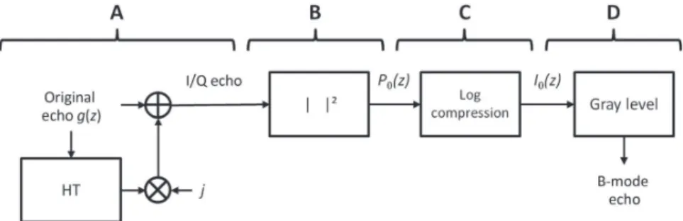
2.1 Background on Ultrasound Imaging and Resolution Quantification Through a Model One of the most common ultrasound imaging representations is known as B-mode. The envelopes of individual signals received from structures to be imaged or RF signals are computed after beamforming, filtered, log-compressed, and, finally, displayed in gray levels (Fig. 1). Given an individual baseband RF echo gðzÞ, its envelope is, thus, defined by:
P0ðzÞ ¼ jgI∕QðzÞj; (2)
with
gI∕QðzÞ ¼ gðzÞ þ jHT½gðzÞ'; (3)
where j2¼ −1 and g
I∕Qis referred to as the complex analytical
signal [or nondemodulated In-phase and Quadrature (I∕Q) sig-nal]. The envelope is obtained through step B of Fig.1and HT½ ' denotes the Hilbert transform used in step A of Fig.1. In step B, the magnitude of gI∕Qis computed. For a real-value narrowband
(echo) signal gðtÞ, the Hilbert transform is defined by:
HT½gðzÞ' ¼ −gðzÞ ⊗ 1
πz; (4)
where⊗ stands for the convolution product. Step C of Fig.1is a log compression and step D is a conversion to gray levels. All the B-mode echoes are then juxtaposed to be displayed as an image. Here, we are interested in post-beamforming imaging.
2.2 Proposed Parametric Spectral Like Super-Resolution Approach
Starting from Eq. (2) giving the B-mode representation, we will show hereafter that an analogy may be done between the envelope estimation and the classical Fourier-based power spec-trum density. In the following, the classical Fourier-based power spectrum density will be referred to as PSD. It is known that the PSD estimates have poor frequency resolution. One main sol-ution to improve the resolsol-ution of the PSD is to use parametric methods, such as AR, to estimate the PSD.13,14
Let us begin by recalling a classical result from parametric AR spectral modeling. The interested reader may refer to, e.g., Refs.13 and14. Let a given real- or complex-number signal yðnÞ defined by N samples be modeled by an AR process. The signal yðnÞ may be rewritten as:
Fig. 1Principle of B-mode imaging. Like the original ultrasound image, which is a collection of gðzÞ echoes, the B-mode image is a collection of B-mode echoes.
blue yðnÞ ¼ −X M i¼1
aiyðn − iÞ þ ωðnÞ; (5)
where M is the number of parameters, also referred to as the model order, ωðnÞ is a zero mean white noise, with variance σ2, and the parameters ai are complex number parameters.
The methodology also stands for nonwhite noise.
From Eq. (5), it can be shown that the PSD is given by:
PSDyðfÞ ¼
σ2 j1 þPM
m¼1amexpð−2πjfmÞj2
; (6)
where j2¼ −1 and f stands for the normalized frequency such that−ð1∕2Þ ≤ f ≤ ð1∕2Þ. From Eq. (6), it can be seen that since PSDyðfÞ is directly linked to the frequency variable f via the
exponential function, the frequency resolution may be theoreti-cally not limited, provided the am coefficients and the model
order M are known. The classical spectral analysis may be resumed as follows. We consider for better readability, without loss of generality, a noiseless signal yðnÞ (when the signal is noisy, the results are valid, the signal is split on some short win-dows, and the PSD is averaged on these windows). To obtain the PSD of a time or space-varying signal yðnÞ, two possible paths exist.
• Path 1: From the time or space-varying signal yðnÞ, first
compute the Fourier transform; then take the magnitude (possibly averaged on short windows) to obtain the PSD, say PðfÞ.
• Path 2: From the time or space-varying signal yðnÞ,
per-form an AR analysis by first estimating the AR parameter aiin Eq. (5); then estimate the PSD using Eq. (6).
It is well known that parametric spectral methods (as com-pared to some classical Fourier spectral analyses) improve the frequency resolution of a PSD estimation. Moreover, it results from Fig.1that the ultrasound B-mode computation is based on the estimation of the envelope image. Thus, obtaining the envelope of an ultrasound signal is very similar to obtaining the classical PSD (path 1). That is, they are the magnitudes of, respectively, the complex analytical signal [Eq. (2)] and the Fourier transform. To improve the resolution of the envelope of an ultrasound signal, we propose to use the AR modeling as in classical spectral (PSD) analysis, by following (path 2) through a domain change.
This is achieved by computing the inverse Fourier transform of the received echo signal. This is explained by the fact that in spectral analysis, the time or space signal and the PSD are in two differents domains (respectively, the time or space domain and frequency domain), whereas in the envelope estimation, the time or space signal and the envelope are in the same domain. Thus, for envelope estimation with AR modeling, we need to change the processing domain so that this processing domain differs from the envelope domain. To do so, we go from the time or space domain to the inverse Fourier domain so that applying AR modeling yields the original time or space domain. The parametric spectral model is, thus, applied to the result of the inverse Fourier transform of the time or space signals, and gives us an estimation of envelope of the ultrasound signal (instead of the PSD). This is the dual part of Eqs. (5) and (6). Equation (5) is in the time or space domain and Eq. (6) in the frequency domain. Thus, performing an inverse Fourier
transform of the RF signal and then using Eqs. (5) and (6) on this inverse Fourier transform leads to a new (better resolved) envelope signal.
The domain change and the super-resolved envelope estima-tion method are further detailed below.
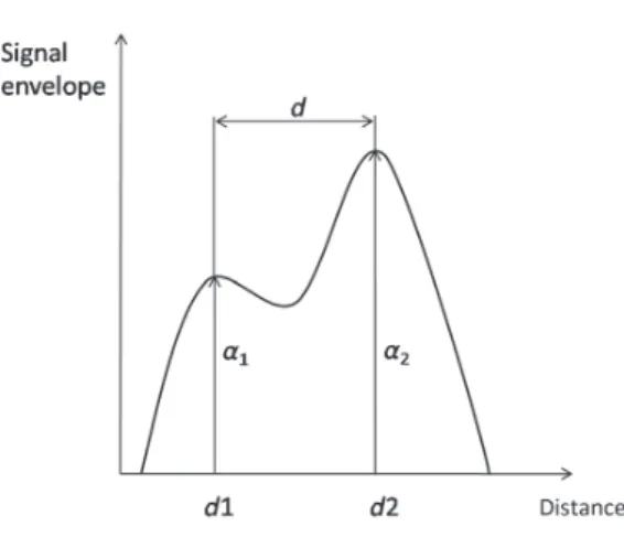
Let us consider the spatial resolution analysis problem and, especially, the evaluation of the resolution. Consider two point objects, separated by a distance d, receiving a beam and reflect-ing ultrasound toward the emittreflect-ing transducer. Assume the PSF of this imaging system is g, and assume its envelope has an abso-lute maximum, causal and zero at infinity.
Also assume all the parameters of the ultrasound imaging system (speed of sound, frequency, attenuation, etc.) are fixed. The two point sources located at d1and d2¼ d1þ d produce
the echoes gðz − d1Þ and gðz − d1− dÞ, respectively (see
Fig.2).
Performing a trivial variable change and sampling above the Nyquist frequency, the received echo signal can be written as:
yðzkÞ ¼ α1g " zkþ d 2 # þ α2g " zk− d 2 # þ wðzkÞ; (7)
where α1and α2denote the uncorrelated random magnitude of
each point and are related to the acoustic properties of the point sources. wðzkÞ is an additive zero mean Gaussian white noise
with variance σ2
w. Each point’s response is, thus, a convolution
of a band-limited PSF envelope with a Dirac peak located at d1¼ −ðd∕2Þ and d2¼ ðd∕2Þ.
Applying the inverse Fourier transform to Eq. (7), we obtain:
YðukÞ ¼ α1GðukÞ exp " −j2πd 2uk # þα2GðukÞ exp " j2πd 2uk # þ WðukÞ: (8)
The AR model is then applied to Eq. (8) to improve the envelope resolution.
In the following, we consider different assumptions:
• The speed of sound is constant over the imaged tissues. • The two point sources are sufficiently close to have the
same attenuation.
• We consider, without loss of generality, that the PSF has a
unit energy.
What we are interested in here is finding a practical way to access the resolution.
Let us summarize the proposed method. From the received ultrasound RF signal yðzkÞ, we first perform an inverse Fourier
transform to obtain YðukÞ, then we apply an AR model using
YðukÞ [that is, we replace yðnÞ in Eq. (5) by YðukÞ instead of
yðzkÞ], and, finally, we estimate the envelope by using Eq. (6) as
shown below: yðzkÞ ! FT−1 YðukÞ ! AR model SARðzÞ;
where zkand z are time or space variables. zkis discrete time (or
space), whereas z is the continuous-time (or space) variable according to Eq. (6); SARðzÞ ∈ Rþ. Instead of providing an
esti-mated PSD, the parametric spectral method gives us SARðzÞ, an
estimated envelope of yðzÞ, thanks to the inverse Fourier trans-form previously computed. SARðzÞ is, thus, a parametric spectral
like an envelope. Note that any other high-resolution spectral analysis method can be used instead of AR modeling, which is used here for convenience and simple derivations.
We now investigate the relevance of the method by analyzing the relationship among the resolution, signal-to-noise ratio (SNR), and the model features.
Let us, thus, define
θ¼ ½a1; a2; : : : ; aM'T: (9)
The estimate of θ will be further denoted by ^θ.
In this context, by ignoring the constant, which is not useful here, Eq. (6) can be rewritten as
SARðzÞ ¼ 1
AðzÞ; (10)
where SARis the super-resolved envelope of the RF signal, and AðzÞ ¼ ð1 − zH^θÞ)
ð1 − zH^θÞ; (11)
where T and H stand, respectively, for the transpose and trans-pose conjugate operators, and
z¼ ½expðjzÞ; expðj2zÞ: : : expðjmzÞ'T: (12)
A practical condition15–17for determining the resolution
abil-ity is analyzing AðzÞ [rather than SARðzÞ] at the center location
of the interval d, i.e., compare Að0Þ with the average of the envelope evaluated at locations d1 and d2. To do so, it is
common to define the quantity
R¼ Að−d∕2Þ þ Aðd∕2Þ − 2 Að0Þ; (13) and the resolution problem comes to the point of hypothesis test-ing:
% R < 0: the two points are resolved
R≥ 0: the two points are not resolved: (14) Actually, the resolution limit case corresponds to
R¼ 0: (15)
From Eqs. (5) and (8), let us define
ϕðuk− 1Þ ¼ ½Yðuk− 1Þ: : : :Yðuk− MÞ'T; (16)
Cy¼ E½ϕðuk− 1ÞϕHðuk− 1Þ'; (17) Ψ ¼ E½ϕðuk− 1ÞY)ðukÞ'; (18) ¯zp¼ ½expðj¯zpÞ; expðj2¯zpÞ: : : expðjM¯zpÞ'T; (19)
with p¼ f1;2; 3g and ¯z1¼ − d 2; ¯z2¼ d 2; ¯z3¼ 0; (20) where Cyis the data covariance matrix. Note that Cyexplicitly
depends on the model order M.
These provide the least square estimate given by ^θ ¼ C−1
y Ψ: (21)
Thus, when ^θ is estimated, R in Eq. (13) can be estimated using Eq. (11). Thus, solving Eq. (15) makes it possible to estab-lish a nonlinear relation among the resolution limit, the SNR, and the model order (see Sec.2.3).
2.3 Resolution Analysis
Here, we perform resolution analysis with respect to the imaging features. For readability, from Eq. (7), we set α1¼ α2, and
SNR¼ α2
1∕σ2win all the following. Here, we perform an analysis
with different kinds of PSF.
2.3.1 Ideal case
First, we consider the ideal case in which we set gðzÞ ¼ δðzÞ in Eq. (7), which means y is wide-band. When y is wide-band, i.e., GðuÞ ∼ 1, an explicit nonlinear expression, can be provided. Indeed, from Eqs. (8) and (17) comes
Cy¼ α21¯zH1¯z1þ α22¯zH2¯z2þ σ2wI: (22) Define τkl¼ ¯zk¯zH l M ; (23)
with k; l∈f1;2; 3g. Using either the matrix inversion lemma or eigenvalue/vector decomposition,16,17it can be shown that R in
Eq. (13) yields RðM; Δ; SNRÞ ¼ jB1j2þ jB2j2− 2jB3j2; (24) where B1¼ β1Mþ β2Mτ12− 1; B2¼ β1Mτ21þ β2M− 1; B3¼ β1Mτ31þ β2Mτ32− 1; β1¼ SNR þ MðSNRÞ2½MðSNRÞðjτ 12j2− 1Þ − ð1 þ τ12Þ' ½MðSNRÞ þ 1'2−½MðSNRÞjτ 12j'2 ; β2¼ SNR þ MðSNRÞ2½MðSNRÞðjτ 12j2− 1Þ − ð1 þ τ21Þ' ½MðSNRÞ þ 1'2−½MðSNRÞjτ 12j'2 :
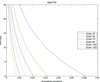
This particular case is similar to the work reported in Ref.17. Solving this nonlinear equation provides the resolution. The results are shown in Fig. 3. Thus, the resolution increases with the model order and the SNR. However, this relation is not clear for a low SNR (<0 dB). This means better resolution may not be achieved for a very low SNR. In practical applica-tions, one does not consider an SNR <0 dB.
2.3.2 Gaussian envelope
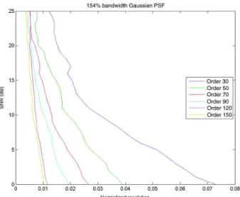
Let us now consider the PSF as gðuÞ ¼ e−ðu2∕2χ2Þ
cosð2πf0uÞ.
We define B¼ ð1∕2πχÞ. The relative (frequency) bandwidth of gis then defined by B∕f0, with f0the center frequency of the
transducer. In ultrasound imaging, this is an important parameter that is used to characterize the transducers.
We consider here relative bandwidths of 30, 50, 100, and 150%. As can be seen in Figs.4–7, the resolution is directly related to the bandwidth and the model order.
The curves in Fig.4have the same shape as in the ideal case, but with a lower resolution for a given SNR.
As expected, the resolution increases when the AR model order increases. Compared to the ideal case, the resolution is globally worse when the band is taken into account.
From this, and by interpolation, we can give a simple empir-ical expression for the resolution distance d:
d¼ KBð1 þ 1∕BÞ θB
SNRθSð1 þ MÞθM; (25)
with KB¼ 0.29; θB¼ 0.25; θS¼ 0.31; θM¼ 0.52. This
expression shows the relation among resolution, SNR, model order, and bandwidth. Typically, for ultrasound systems, the bandwidth is constant. So the higher the order, the better is the resolution. However, an optimal order should be chosen to avoid artifacts.
Fig. 3 Signal-to-noise ratio (SNR) versus resolution and order for an ideal point spread function (PSF). The SNR goes from 25 dB at the top to −30 dB for the bottom line.
Fig. 4 SNR versus resolution and order for a Gaussian PSF of 30% relative bandwidth.
Fig. 5 SNR versus resolution and order for a Gaussian PSF of 50% relative bandwidth.
Fig. 6 SNR versus resolution and order for a Gaussian PSF of 100% relative bandwidth.
2.3.3 Nonsymmetric ultrasound echo
In ultrasound imaging, ultrasound is emitted through a pulse which is not symmetrical. In this section, we, hence, use a nonsymmetric PSF in order to more closely approximate the medical ultrasound imaging conditions. In this case, based on the example in Sec. 2.3.2, the PSF is assumed to be gðuÞ ¼ u3e−ðu2∕2χ2Þ
cosð2πf0uÞ, see Fig.8.
The results in Fig.9are similar to the Gaussian envelope case. This confirms the relationship among the resolution, model order, and bandwidth of the system (PSF).
The relationship between AR model order and the character-istics of the transducer PSF is direct but nonlinear. This relation suggests that finding the order is an important issue for the res-olution improvement of an ultrasound image processed using an AR model. A solution is provided in the following sections with the practical application to ultrasound images.
3
Ultrasound Radio Frequency Signal
Processing
3.1 New Multidimensional Instrumental Matrix Estimation Technique
As stated above, the B-mode ultrasound image consists of RF line envelopes. In order to increase the resolution of B-mode images, these envelopes have to be improved. In this study, instead of directly estimating the envelopes of the RF signals, we used specific AR modeling to achieve this via the inverse Fourier transform of analytical signal gI∕QðzÞ introduced in
Eq. (3). In the following, we will dentote it by y.
Let us consider a second-order stationary multidimensional complex AR process (ND-AR) defined as follows:
yðn1; n2; : : : ; nNÞ ¼ X ðk1;k2;: : : ;kNÞ∈I X aðk1; k2; : : : ; kNÞ ×yðn1− k1; n2− k2; : : : ; nN− kNÞ þ wðn1; n2; : : : ; nNÞ; (26) where wðn1; n2; : : : ; nNÞ is a field of random colored or
corre-lated noise, and the parameters aðk1; k2; : : : ; kNÞ are complex
numbers and provide a stable system. We consider here an ND-model to make our method general and applicable to three-dimensional (3-D) or four-three-dimensional (4-D) images. As in Ref. 18, we focus on the first hyperplane model without loss of generality. The methodology may be applied to other hyper-planes, i.e., the set of neighbors is I¼ fðk1; k2; : : : ; kNÞj
ki¼ 1;2; : : : ; pi; i¼ 1;2; : : : ; Ng. For convenience, we
assume that p1¼ p2¼ : : : pN¼ m, meaning that the model
orders are identical in all directions. The well known one-dimen-sional (1-D) instrumental variable technique is a simple and effi-cient way to overcome basic least-square estimations, which are biased in the presence of colored noise or correlated data.13We propose here a generalization of the 1-D case to a multidimen-sional structure based on UDVH factorization, allowing access
to recursive estimates of parameters of orders 0 to m. The approach is based on investigating multiple-dimensional signals through long vectors, which makes it very simple. In addition,
Fig. 7SNR versus resolution and order for a Gaussian PSF of 150% relative bandwidth. 0 10 20 30 40 50 60 70 80 90 100 3 2 1 0 1 2 3
Fig. 8 Example of an asymmetric echo function for g.
Fig. 9 SNR versus resolution and order for symmetrical and nonsym-metrical PSF.
the algorithm is defined for complex numbers. First, we define the following vectors where elements of y and a are stacked: ϕT mðn1; n2; : : : ; nNÞ ¼ ½yðn1; n2; : : : ; nN− 1Þ: : : yðn1; n2; : : : ; nN− mÞ: : : yðn1; n2− 1; : : : ; nNÞ: : : yðn1; n2− m; : : : ; nNÞ: : : yðn1− m; n2− m; : : : ; nN− mÞ: : : yðn1; n2; : : : ; nNÞ%; (27) θT mðn1; n2; : : : ; nNÞ ¼
½að0;0; : : : 1; Þ: : : að0;0; : : : mÞað0;1; : : : 0; Þ: : :
að0; m; : : : 0; Þ: : : aðm; 0; : : : ; 0Þ: : : aðm; m; m: : : mÞ: : : 1%: (28) Note that yðn1; n2; : : : ; nNÞ and 1 are parts of these vectors.
Defining xT mðn1; n2; : : : ; nNÞ ¼ ½yðn1; n2; : : : ; nN− 1Þ: : : yðn1; n2; : : : ; nN− mÞ: : : yðn1; n2− 1; : : : ; nNÞ: : : yðn1; n2− m; : : : ; nNÞ: : : yðn1− m; n2− m; : : : ; nN− mÞ% (29) means that ϕT mðn1; n2; : : : ; nNÞ ¼ ½xTmðn1; n2; : : : ; nNÞyðn1; n2; : : : ; nNÞ%: (30) The instrumental data structure can be defined as
ζT mðn1; n2; : : : ; nNÞ ¼ ½zðn1; n2; : : : ; nN− 1Þ: : : zðn1; n2; : : : ; nN− mÞ: : : zðn1; n2− 1; : : : ; nNÞ: : : zðn1; n2− m; : : : ; nNÞ: : : zðn1− m; n2− m; : : : ; nN− mÞ: : : zðn1; n2; : : : ; nNÞ%: (31) Different approaches can be used to select the instrument z, see, e.g., Ref.19, for example, a solution consists of introducing a delay for each component of x.
ψT
mðn1; n2; : : : ; nNÞ ¼ ½ζTmðn1; n2; : : : ; nNÞzðn1; n2; : : : ; nNÞ%: (32) Defining the data regression matrix as
Pmðn1; n2; : : : ; nNÞ ¼ X n1 i1¼1 : : : X nN iN¼1 ψmðn1; n2; : : : ; nNÞϕHmðn1; n2; : : : ; nNÞ "−1 (33) and assuming that p¼ ðm þ 1ÞN, the size of this matrix is
p × p. For convenience, the following notations can be used when no confusion is possible:
• n¼ ðn1; n2; : : : ; nNÞ
• k¼ ðk1; k2; : : : ; kNÞ
• and more generally, for any index variableðt1; t2; : : : ; tNÞ:
t¼ ðt1; t2; : : : ; tNÞ. In addition, we denote • Pni¼1instead of Pn1 i1¼1: : : PnN iN¼1
• Pn−ii¼1instead of
Pn1−i i1¼1: : :
PnN−i iN¼1.
We can then write Pm in its factorized form as follows: PmðnÞ ¼ UmðnÞDmðnÞVHmðnÞ; (34)
whereð ÞHdenotes the Hermitian matrix transpose. The
differ-ence between this and the case presented in Ref.18is that the noise considered in Eq. (26) is a colored or correlated noise. Thus, through instrumental data as in Eq. (31), we used a matrix decomposition such as in Eq. (34) in which U≠ V (taking U¼ Vwould have resulted in biased parameter estimates, as in the case of classical estimation theory). As in Eq. (34), U is an upper triangular matrix with all its diagonal elements equal to one. The elements of this upper triangular matrix are column vectors of dimensions 1 to p defined as follows:
UmðnÞ ¼ ½ 1 colf ϑ0;pðnÞ 1 g : : : colf ϑp−i;iðnÞ 1 g : : : colf ϑp−1;1ðnÞ 1 g : : : colf ϑp;0ðnÞ 1 g %: (35)
Remark:
• ϑp−i;iðnÞ is a column vector of dimension p − i.
• colf ϑp−i;iðnÞ 1 g ¼ ϑp−i;iðnÞ 1 " is the ðp − i þ 1Þ’th column.
• Due to the model structure in Eq. (28), ϑp−i;iðnÞ consists
of parts or all of the instrumental variable estimates of the true parameters of the model, depending on whether the model order is smaller or larger than the dimension of ϑp−i;iðnÞ.
Similarly, V is an upper triangular matrix with all its diagonal elements equal to one. The other elements of V are different from those of U. These elements are the intermediate variables necessary to obtain the matrix decomposition. They also consist of column vectors of dimensions 1 to p, defined as follows: VmðnÞ ¼ ½ 1 colf χ0;pðnÞ 1 g : : : f χp−i;iðnÞ 1 g : : :
colf χp−1;1ðnÞ 1 g : : : f χp;0ðnÞ 1 g %: (36)
DmðnÞ in Eq. (34) is a diagonal matrix. Equation (34) is
obtained from successive decompositions. Using Eq. (30) in Eq. (33), we obtain P−1mðnÞ ¼ Pn j¼1ζmðjÞxHmðjÞ Pn j¼1ζmðjÞyðjÞ Pn j¼1zðjÞxHmðjÞ Pn j¼1 Pn j¼1yðjÞzðjÞ " : (37) The methodology developed in Ref.18may be used to esti-mate the matrices U, V, and D, and select the estiesti-mated param-eters and orders of the model presented in Eq. (26). The difference here is that the elements of D are generalized loss functions for orders 1 to m. The first component of D is then:
Jp;0ðnÞ ¼ Xn j¼1 ½yðjÞ − ^yðjÞ%½zðjÞ − ^zðjÞ%; (38) where ^yðnÞ ¼X n j¼1 xH mðjÞϑp;0ðnÞ ^zðnÞ ¼ Xn j¼1 zH mðjÞχp;0ðnÞ
and its p− i column is:
Jp−i;iðnÞ ¼ Xn j¼1
½yðjÞ − ^yðjÞ%½zðjÞ − ^zðjÞ%.
Note that the result of this last equation is a complex number. By taking its magnitude value, a cost function is provided. Also, note that all elements of the matrices are stacked and Dm has
ðm þ 1ÞN×ðm þ 1ÞN elements. Thus, to find the true order
of the model, the following steps may be used:
1. Split elements of Dminto successive segments of mþ
1 elements, and create a new vector, M1, consisting of
the minima of the segments.
2. Repeat step 1 using the above set of minima. 3. Stop when the size of the vector of minima is mþ 1.
This vector is called MN. This procedure needs
N steps.
4. Finally, the minimum of MNgives the true order m0.
Depending on the organization of xH
mðnÞ in Eq. (29), the true
parameters may be accessed following the methodology devel-oped in Ref.18. The decomposition of Eq. (34) may be per-formed by batch, or recursively. In this last case, the main step of the recursion is defined as follows. From Eq. (33), it can be written as
PmðnÞ ¼ ½P−1mðn − 1Þ þ ψmðnÞϕHmðnÞ%−1: (39)
The variables can be defined as follows: f1¼ UTmðn − 1ÞϕmðnÞ f2¼ VTmðn − 1ÞψmðnÞ g1¼ Dmðn − 1Þf)1 g2¼ Dmðn − 1Þf)2 βðnÞ ¼ 1 þ fT 1g2;
where the asterisk denotes the complex conjugate. PmðnÞ can
now be expressed by: PmðnÞ ¼ UmðnÞDmðnÞVHmðnÞ ¼ Umðn − 1Þ Dmðn − 1Þ − g2gH1 βðnÞ " VH mðn − 1Þ: (40)
From these recursions, only elements of Um with physical
meanings are retained.
The choice of model order is highly important: the higher the order, the better is the resolution; this is also the case for noise artifacts. Thus, this methodology makes it possible to simultane-ously access the order and the parameters of the N− D AR model.
3.2 Improvement of Ultrasound Image Resolution
3.2.1 Power spatial density
We consider the model described by Eq. (26) with N¼ 2. We also recall13,14that the PSD is defined in the first quadrant by
Par1ðf1; f2Þ ¼ σ2 1ðf1; f2Þ jA1ðf1; f2Þj2 ; where A1ðf1; f2Þ ¼ X p1 k1¼0 X p2 k2¼0 a1½k1; k2%e−j2πðf1k1þf2k2Þ; (41)
and in the fourth quadrant by Par4ðf1; f2Þ ¼ σ24ðf1; f2Þ jA4ðf1; f2Þj2 where A4ðf1; f2Þ ¼ X p1 k1¼0 X0 k2¼−p2 a4½k1; k2%e−j2πðf1k1þf2k2Þ: (42) To account for the causality and due to the equivalence between planes,13the overall PSD is:
Par1;4ðf1; f2Þ ¼
σ2ðf1; f2Þ 1
2½jA1ðf1; f2Þj2þ jA4ðf1; f2Þj2%
; (43)
where jA1ðf1; f2Þj2and jA4ðf1; f2Þj2are the denominators in
Eqs. (41) and (43). We used the parametric modeling developed in Sec.3.1to estimate the model parameter. Instead of the PSD, we obtained an image envelope estimate which is equivalent to PSD. Thus, to improve the spatial resolution, we applied this technique to the inverse Fourier transform of the demodulated
Fig. 10 Cost function: the curve shows the loss function after extrac-tion of the minima. As can be seen, the minimum is achieved for m0¼ 2.
I/Q signal given by the RF signals. Our methodology can, thus, be summarized as follows:
1. Obtain the Fourier transform of the nondemodulated I/ Q signal in order to be in the Fourier domain. 2. Perform parametric modeling (using the approach
pro-posed in Sec.3.1).
3. Then estimate PSD and get an envelope of the demodulated I/Q signal with better resolution.
4
Results
4.1 Example of N-D Model Order and Parameters Estimation
To illustrate the method presented through Eqs. (26) to (40), we set N¼ 2, since our aim is to deal with images, m ¼ 4 and
m0¼ 2. We consider the following two-dimensional (2-D)
com-plex AR model as defined in Eq. (28), where the model param-eters aðk1; k2Þ, k1¼ 0;1; 2; k2¼ 0;1; 2 are defined as follows.
að0;0Þ ¼ 1 is not estimated.
yðn1; n2Þ ¼ X2 k1¼0 X2 k2¼0;ðk1;k2Þ≠ð0;0Þ aðk1; k2Þyðn1− k1; n2− k2Þ þ wðn1; n2Þ;
with wðn1; n2Þ ¼ eðn1; n2Þ þ ð1 þ 3iÞeðk1− 1; k2Þ, where y is
a 64 × 64 complex field driven by a complex colored noise wðn1; n2Þ obtained via eðn1; n2Þ, a Gaussian random field
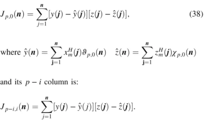
with variance 0.1. Following the same order determination as in Ref. 18, we find an order of 2, as can be seen in Fig.10. The parameter estimates are shown in Table1.
4.1.1 Application to ultrasound images
The proposed method was applied to simulation (Fig. 11), in vitro(Fig.13) and in vivo images (Fig.14). For our simulation, we first generate a synthetic ultrasound image, representing a homogeneous medium crossed by a vessel, using the Field II simulation program.20The simulation parameters were as fol-lows: central frequency = 3 MHz, number of RF lines simulated = 256, number of scatterers = 10,000. Then we generate the same image at a central frequency = 6 MHz, in order to double the image spatial resolution. The 3 MHz image was processed using our approach and the result was compared with the 6 MHz image. As can be seen qualitatively, the results are close to Fig.11, last row (from top to bottom). Moreover, a profile of the envelope is extracted from the same RF lines of these images. As can be seen in Fig. 12, the profile obtained from
Table 1 Theoretical parameters (top) and estimated parameters (bottom) aðk1; k2Þ.
1 −1.0000 − 1.0000i 0.0625þ 0.5000i −1.0000 − 1.0000i 0þ 2.0000i 0.4375 − 0.5625i 0.0625þ 0.5000i 0.4375 − 0.5625i −0.2461þ 0.0625i
1 −1.0049 − 1.0022i 0.0632þ 0.4833i −1.0477 − 1.0386i 0.0031þ 2.0308i 0.4373 − 0.5749i 0.0528þ 0.5580i 0.4524 − 0.5728i −0.2447þ 0.0699i
Fig. 11 Comparison between synthetic original and processed images: (a) original 3 MHz image, (b) 6 MHz image, which is the ground truth, and (c) the processed image obtained from the original 3 MHz image, with our method.
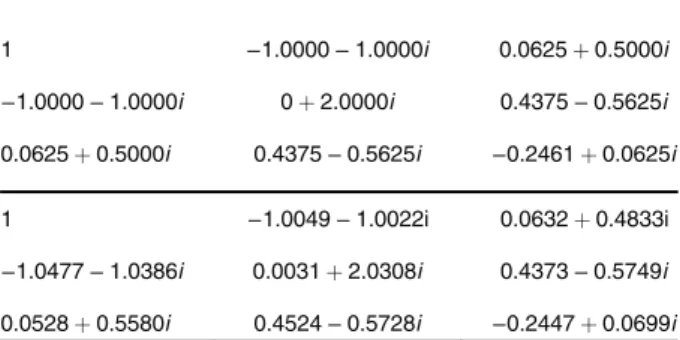
our approach is close to that of the 6 MHz image. Figure13
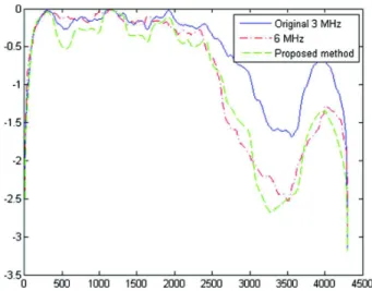
shows, for illustration purposes, the results on an in vitro image using a phantom made of a thread embedded in a gel. To give an indication of what an expected synthetic image should look like, the theoretical image is arbitrarily drawn and shown at the top of Fig. 13. The bottom-left image is the original 20 MHz ultrasound image, and the bottom right shows the resulting image after using the proposed method. The processed image is closer to the expected theoretical image. We also show, in Fig.14, the results on an in vivo ultra-sound image of, from top to bottom, the bladder of a mouse (first row), a rabbit eye (second row), the uterus of a pregnant mouse (third row), and a simulation image (fourth row). Qualitatively,
as can be seen in each processed image, the edges are sharpened by the processing technique, which indicates that the spatial res-olution has been improved. For spatial resres-olution estimation, we use Eq. (25). From this equation, we can compute the improve-ment in resolution. Given an image and device characteristics, this equation empirically indicates the theoretical minimal achievable resolution. This resolution depends on the SNR, model order, and bandwidth of the ultrasound probe. From images in Fig. 14, we performed 1-D analysis on individual RF lines of the images. The estimated axial bandwidth of the PSF of the probe used to obtain images in Fig. 14(first three rows) was 60%. In Table 2, for these images, we evaluated the improvement in resolution defined by the ratio
Rest∕Ract;
where Ractis the actual resolution [Eq. (1)] for the ultrasound
frequency f0and Restis the a posteriori resolution estimated by
our approach. Note that this ratio should be <1 to show tion enhancement. The theoretical axial improvement in resolu-tion obtained for Fig.14, from top to bottom, first row, second row, third row, and fourth row, is, respectively, 0.9, 0.7, 0.6, and 0.5, as is shown in Table2. To evaluate the improvement in lat-eral resolution, we also performed a 2-D analysis. For the images in Fig.13, the estimated bandwith in the axial direction was 60% and that in the lateral direction was 11%. The orders found in axial and lateral directions were respectiveley 5 and 5. The axial and lateral resolution improvements were 0.6 and 0.3, respectively. We also compared our technique to classical ones, namely, homomorphic filering, e.g., Ref. 7, and parametric inverse filtering via hybrid approach (HYPIF) filtering.8 For
this comparison, we used the classical gain in resolution param-eter, e.g., Refs.8and9, since these methods do not allow the estimation of the improvement in resolution introduced here. The results are shown in Table3. As can be seen, our technique
Fig. 12 Comparison between profiles: profiles of the log-envelope of an extracted radio frequency line located in the top of Fig.11(solid line) from the synthetic 3 MHz image (solid), the synthetic 6 MHz image (dash dot), and processed images (dash).
Fig. 13 Comparison between the expected theoretical image (a), the original ultrasound image of a phantom consisting of a thread embedded in a gel (b), and the processed image (c) obtained from the original ultrasound image. The thread edge is sharper on the processed image.
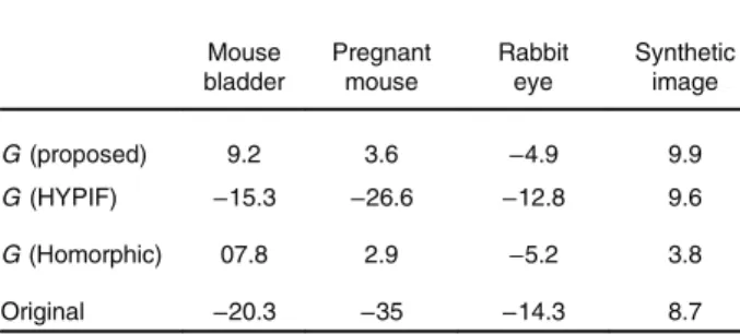
outperforms these methods. Moreover, although the primary goal of the proposed method was not to enhance the contrast (but the resolution), we also compare our method with the existing methods in terms of contrast-to-noise ratio (CNR), see, e.g., Ref.21. The CNR is defined as
CNR¼ jμffiffiffiffiffiffiffiffiffiffiffiffiffiffiffi1− μ2j σ2
1þ σ22
p ;
where μ1, μ2, σ1, and σ2are, respectively, the mean and the
vari-ance of the pixels in two chosen regions of interest highlighted by the square boxes in Fig.14. The higher the CNR, the better is the contrast. As can be seen in Table4, even if the CNR is not high for all the images, our method outperforms the existing ones in all the cases. Finally, Table5shows the computation times of the different methods for an image of size 1024 × 256, using a 2.1 MHz dual core Xeon PC. As can be
Fig. 14 Comparison of visual appreciation of different methods on different images. From left to right, first column: the original images, second column: the results for homorphic filtering, third column: the results for HYPIF, and fourth column: the results of the proposed method. From top to bottom, first row: a mouse bladder image, second row: rabbit eye image, third row: uterus of a pregnant mouse, and fourth row: a synthetic image.
Table 2 Improvement in resolution. The bandwidth of the used trans-ducer was 60% except for the simulation one, which was 90%.
Mouse bladder
Pregnant
mouse Rabbit eye
Synthetic image f0¼ 20 MHz f0¼ 20 MHz f0¼ 20 MHz f0¼ 3.5 MHz Found order 79 82 70 70 Rest∕Ract 0.9 0.6 0.7 0.5
Table 3 Empirical gain in resolution.
Mouse bladder Pregnant mouse Rabbit eye Synthetic image G (proposed) 11.97 2.76 4.20 3.71 G (HYPIF) 1.1 1.26 1.16 0.49 G (Homorphic) 1 0.99 1.00 0.36 G 3.5 MHz versus 7 MHz — — — 1.5
seen, the computation time of our method is reasonably low (although higher than the one of homomorphic filtering).
5
Conclusion and General Remarks
In this work, we first revisited super-resolution theory in the framework of ultrasound imaging. The improvement of resolu-tion can be quantified, given the PSF shape, the SNR, and the AR model order. For better readability, all results and deriva-tions were presented in 1-D. Then we presented a way to improve ultrasound image resolution. The methodology devel-oped is based on specific spectral analysis like modeling, which fits ultrasound images. Applied to synthetic, in vitro, and in vivo images, this methodology shows a qualitative and quantitative resolution improvement. An important characteristic of the pro-posed approach is its ability to estimate a priori the improve-ment in resolution. The improveimprove-ment in resolution achieved here is up to a ratio of two. To our knowledge, this work is the first to deal with the a priori estimation of the gain in res-olution in ultrasound imaging. Finally, comparisons with existing techniques were provided. The results show that the proposed method outperforms existing techniques, both in terms of subjective visual quality and in terms of quantitative evaluation using the classical gain in resolution. Although we focus here on the 1-D and 2-D cases and show improvement of the resolution of ultrasound images using the proposed method, the methodology proposed may be applied whatever be the imaging processing dimension (3-D or 4-D).
Acknowledgments
This work was supported by ANR-11-LABX-0040-CIMI within the program ANR-11-IDEX-0002-02 of the University of Toulouse.
References
1. L. Rayleigh, “On the manufacture and theory of diffraction-gratings,” Philos. Mag. 47, 193–205 (1874).
2. S. issue, “Special issue on novel equipment for ultrasound research,”
IEEE Trans. Ultrason. Ferroelectr. Freq. Control53 (2006). 3. E. Filoux, J. Mamou, and O. A. J. Ketterling, “Characterization of the
spatial resolution of different high-frequency imaging systems using a
novel anechoic-sphere phantom,”IEEE Trans. Ultrason. Ferroelectr. Freq. Control58, 994–1005 (2011).
4. G. Clement, J. Huttunen, and K. Hynynen, “Superresolution ultrasound imaging using back-projected reconstruction,”J. Acoust. Soc. Am.118, 3953–3960 (2005).
5. P. Blomgren and G. Papanicolaou, “Super-resolution in time reversal acoustics,”J. Acoust. Soc. Am.111, 230–248 (2002).
6. F. S. Foster et al., “Advances in ultrasound biomicroscopy,”Ultrasound Med. Biol.26, 1–27 (2000).
7. R. Jirik and T. Taxt, “High-resolution ultrasonic imaging using two-dimensional homomorphic filtering,” IEEE Trans. Ultrason. Ferroelectr. Freq. Control53, 1440–1448 (2006).
8. O. Michailovich and A. Tannenbaum, “Blind deconvolution of medical ultrasound images: a parametric inverse filtering approach,” IEEE Trans. Image Process.16(12), 3005–3019 (2007).
9. U. R. Abeyratne et al., “Higher order versus second order statistics in ultrasound image deconvolution,”IEEE Trans. Ultrason. Ferroelectr. Freq. Contol44, 1409–1416 (1997).
10. J. Ng et al., “Wavelet restoration of medical pulse-echo ultrasound images in an EM framework,” IEEE Trans. Ultrason. Ferroelectr. Freq. Control54, 550–568 (2007).
11. D. Kouame and M. Ploquin, “Super-resolution in medical imaging: an illustrative approach through ultrasound,” in IEEE Int. Symp. on Biomedical Imaging, Boston, Massachusetts, pp. 249–252, IEEE (2009).
12. M. Ploquin and D. Kouame, “Improvement of medical image resolution using an extended 2d factorized form complex number parametric model,” in 17th IEEE Int. Conf. on Image Processing, Hong Kong, pp. 601–604, IEEE (2010).
13. S. M. Kay, Modern Spectral Estimations, Prentice-Hall (1988). 14. S. Marple, Digital Spectral Analysis with Applications, Prentice-Hall
(1987).
15. C. Zhou, F. Haber, and D. Jaggard, “A resolution measure of music algorithm and its application to plane wave arrivals contaminated by coherent interference,” IEEE Trans. Signal Process. 39, 454–463 (1991).
16. Q. Zhang, “A spatial resolution theory of the ar method of spectral analysis,” IEEE Trans. Signal Process. 46, 2757–2766 (1998). 17. S. L. Marple, “Frequency resolution of Fourier and maximum entropy
spectral estimates,”Geophysics47, 1303–1307 (1982).
18. D. Kouamé and J. Girault, “Multidimensional multiple-order complex parametric model identification,” IEEE Trans. Signal Process. 56, 4574–4582 (2008).
19. T. Soderstrom and P. Stoica, “Comparison of some instrumental variable methods—consistency and accuracy aspects,”Automatica17, 101–115 (1981).
20. J. A. Jensen and N. B. Svendsen, “Calculation of pressure fields from arbitrarily shaped, apodized, and excited ultrasound transducers,”JASA
111, 230–248 (2002).
21. P. Stetson, F. Sommer, and A. Makovski, “Lesion contrast enhancement in medical ultrasound,”IEEE Trans. Med. Imaging16, 416–425 (1997).
Marie Ploquin received her MS in 2007 from the University of Tours, Tours, France, and PhD degrees in 2011, in signal and image processing, from the Universities of Tours and Toulouse, France. She is currently a senior engineer at Solent France.
Adrian Basarab received MS and PhD degrees in signal and image processing from the National Institute for Applied Sciences of Lyon, France, in 2005 and 2008. Since 2009, he has been an assistant pro-fessor at the University Paul Sabatier Toulouse 3 and a member of IRIT Laboratory (UMR CNRS 5505). His research interests include medical imaging, and more particularly motion estimation, inverse problems, and ultrasound image formation.
Denis Kouamé is with University Paul Sabatier, Toulouse, France. His research interests are focused on signal and image processing with applications to medical imaging and particularly ultrasound imag-ing, including high resolution imagimag-ing, image resolution enhance-ment, doppler signal processing, detection and estimation with application to cerebral emboli detection, multidimensional parametric modeling, spectral analysis, Inverse problems related to compressed sensing, and restoration.
Table 4 Contrast-to-noise ratio in decibels. The higher, the better.
Mouse bladder Pregnant mouse Rabbit eye Synthetic image G (proposed) 9.2 3.6 −4.9 9.9 G (HYPIF) −15.3 −26.6 −12.8 9.6 G (Homorphic) 07.8 2.9 −5.2 3.8 Original −20.3 −35 −14.3 8.7
Table 5 Computation time (in seconds) for an image of size 1024 × 256.
Method Homomorphic HYPIF Proposed Computation time (s) 0.04 185.40 0.71