Characterizing capital and operational tradeoffs resulting from fiber-to-the-home optical network architecture choice

CHARACTERIZING CAPITAL AND OPERATIONAL TRADEOFFS

RESULTING FROM FIBER-TO-THE-HOME OPTICAL NETWORK

ARCHITECTURE CHOICE

by

Thomas Rand-Nash

B.A in Physics, University of California, Berkeley, 2005

Submitted to The Engineering Systems Division and

The Department of Materials Science & Engineering

in Partial Fulfillment of the Requirements for the Degrees of

Master of Science in Technology and Policy

and

Master of Science in Materials Science and Engineering

at the

Massachusetts Institute of Technology

June 2009

© 2009 Massachusetts Institute of Technology.

All rights reserved.

ARCHIVES

JUL 2

8

2009

LLBRAR7F' I

Signature of Author....

Tecoh

gy

d Policy Program, Engineering Systems Division,

Materials Science and Engineering,

Submitted 5/15/09; Defended 5/21/09

Certified

by...

... ...

...

.

...

...

Richard Roth

Director, Materials Systems Laboratory

Thesis Supervisor

Certified

by... ....

... ..

... ...

...

.

...

"

/

ZRandolph

Kirchain

As ciate Professor of Engineering Systems and Materials Science and Engineering

_

Thesis Supervisor

Accepted by

... ...

.... ...

.... ...

Dava Newman

Profe-sor bfAerona

s

and Astronautics and Engineering Systems

Director, Technology and Policy Program

Accepted by

...

.. ...

...

Christine Ortiz

Chair, Departmental Committee on Graduate Students

CHARACTERIZING CAPITAL AND OPERATIONAL TRADEOFFS

RESULTING FROM FIBER-TO-THE-HOME OPTICAL NETWORK

ARCHITECTURE CHOICE

By

Thomas F. Rand-Nash

Submitted to the Engineering Systems Division and the Department of Materials Science and

Engineering on May 15, 2009 and defended on May 21, 2009 in Partial Fulfillment of the

Requirements for the Degrees of Master of Science in Technology and Policy and

Master of Science in Materials Science and Engineering

Abstract

This thesis explores the impact of relative lifecycle cost tradeoffs on technology strategy, and

characterizes two factors driving these costs: population demographics, and uncertainty in

component costs. The methodology developed consists of three novel components which address

gaps in the current literature in the areas of large-scale network design, multi-attribute population

characterization, and cost modeling. Three technologies representing near, mid, and long-term

fiber-to-the-home gigabit passive optical network solutions, and seven implementation strategies

are dimensioned for two significantly different population demographics, each representing large

coverage regions containing millions of subscribers. The methodology is able to successfully

characterize how relative network topologies changed as a function of population attributes,

revealing complex cost tradeoffs between technology strategies

Thesis Supervisors:

Dr. Richard Roth

Director, Materials Systems Laboratory

Dr. Randolph Kirchain

Acknowledgements

I cannot express in words my gratitude to my advisors, and my group-as they have impacted

my life in ways which defy explanation. Prior to arriving at MIT, I had not enjoyed the comforts

of family in many years; when I leave however, I feel that I will never be without one again. I

have been privileged to learn for a living for the past four years, something very few get to enjoy

for even a day. For this alone I would be grateful. However, to be surrounded by people whose

curiosity is never limited by ability, and who push me to try and find that within myself, has been

a humbling and extraordinary experience. You know who you are: Thank You.

TABLE OF CONTENTS

1 INTRODUCTION ... 11

1.1 PASSIVE OPTICAL N ETWORK OVERVIEW ... ... 12

1.2 OVERVIEW OF TECHNOLOGY CHOICES MODELED ... ... 15

1.3 T H ESIS O U TLIN E ... ... ... 17

2 CURRENT MODELING APPROACHES ... 17

2.1 N ETW ORK M ODELING APPROACHES... 18

2.1.1 Bottom-Up Optimization Approaches... 18

2.1.2 Top-Down Engineering-Rule-Based Approaches ... 19

2.1.3 Network Modeling Approach Comparison and Gap Analysis ... 20

2.2 POPULATION CHARACTERIZATION APPROACHES... ... 21

2.2.1 Population Characterization Gap Analysis... ... 22

2.3 COST M ODELING A PPROACHES... 22

2.3.1 Cost M odeling Gap Analysis ... 23

3 EXPECTED CONTRIBUTIONS ... 23

4 METHODOLOGICAL OVERVIEW ... 24

5 MSL POPULATION CHARACTERIZATION... 25

5.1 POPULATION DENSITY ... 26

5.2 POPULATION DENSITY MODELING ... 27

5.2 .1 D y nam ic G rids... 2 8 5.2.2 Calculating Probability Functions... 29

5.2.3 G rid C ell S ize... ... 29

5.2.4 Grid Cell Spacing ... ... ... 30

5.2.5 Grid Cell Size, Spacing, and Density Constraints ... 30

5.3 H OU SEHOLD D EN SITY ... ... ... 35

5.4 DATA DENSITY... 41

6 MATERIALS SYSTEMS LAB (MSL) NETWORK MODEL ... ... 42

6.1 NETWORK DESIGN M ODEL INPUTS ... 43

6.1.1 Technological Constraints ... ... ... 43

6.1.2 Operating Context... ... ... ... ... 44

6.2 NETW ORK DESIGN M ODEL ALGORITHMS... 44

6.2.1 Neighborhood Size and Frontage Fiber Length... ... 46

6.2.2 Central Office Siting and Neighborhood Assignment ... 49

6.2.3 Splitter Siting & Fiber Link Length Determination ... ... ... 51

6.2.3.1 C onstraint D erivation ... ... 52

6 .2 .3 .2 Sp litter S iting ... 53

7 HEURISTIC CALIBRATION AND SENSITIVITY ANALYSIS ... 59

7.1 POPULATION DEMOGRAPHICS M ODELED ... ... 60

7.2 TECHNOLOGY CHOICE MODELED ... 60

7.3 M ETHODOLOGY... ... ... 61

7.4 R ESULTS AN D A NALY SIS ... 62

8 COST MODELS ... 65

8.1 CAPEX MODEL ... 66

8.2 OPEx MODEL ... ... 67

9 METHODOLOGY VALIDATION, DEMONSTRATION, AND LIMITATIONS ... 70

9.1 NETWORK MODEL INTERNAL CONSISTENCY ANALYSIS... 71

9.1.1 M ethodology ... ... ... ... 71

9.2 NETWORK MODEL BENCHMARKING ... 74

9.2.1 BT Validation Study ... ... 74

9.2.1.1 T echnology M odeled ... ... 74

9.2.1.2 Population M odeled ... ... 75

9.2.1.3 R esults and A nalysis ... ... 76

9.2.2 Corning Study Validation ... 76

9.2.2.1 Technology Choice M odeled... ... 77

9.2.2.2 Population M odeled ... ... 77

9 .2 .2 .3 M etho do logy ... ... ... 80

9.2.2.4 Results ... ... 88

9.2.3 Benchmarking Exercise Conclusion ... ... 89

9.3 NETWORK MODEL LIMITATIONS... 89

9.4 CAPEX MODEL VALIDATION ... 89

9.5 CAPEX MODEL CAPABILITIES ... 91

9.6 CAPEX MODEL LIMITATIONS ... 94

9.7 OPE MODEL CAPABILITIES ... 95

9.8 OPE MODEL LIMITATIONS ... 97

10 CASE STUDY ANALYSES ... 97

10.1 M ETHOD OLO GY ... 97

10.2 TECHNOLOGY CHOICES / IMPLEMENTATION STRATEGIES MODELED ... 98

10.3 BASE CASE ... ... 99

10.3.1 Population Demographic Profiles Modeled... 100

10.3.2 Region I: High Population Density /High Data Demands... 101

10.3.3 Base Case Results and Analysis ... ... 105

10.4 EFFECTS OF PENETRATION AND DISCOUNT RATE ON TECHNOLOGY STRATEGY ... 111

10.4.1 High-Density, High Data Demand Population Results ... 112

10.4.2 Low Density, Low Data Demand Population Results... 114

10.5 EFFECTS OF UNCERTAINTY IN FUTURE TECHNOLOGY COSTS ON TECHNOLOGY STRATEGY... 116

10.5.1 M ethodology ... 116

10.5.2 Results and Analysis... 117

10.5.3 Low-Density, Low Data Demand Population Results ... 118

10.5.4 High-Density, High Data Demand Population Results ... 122

11 CONCLUSIONS AND CONTRIBUTIONS ... 124

11.1 CONCLUSIONS ... ... 124

11.2 C ON TRIBU TION S... ... 125

12 CARRIER RECOMMENDATIONS ... 126

13 FUTURE W ORK ... ... 126

TABLE OF FIGURES

FIGURE 1: BASIC GPON NETWORK ARCHITECTURE ... ... 13

FIGURE 2: M ODELING O VERVIEW ... ... ... 25

FIGURE 3: SAMPLE 100KM2 COVERAGE REGION WITH THREE POPULATION DISTRIBUTIONS ... 26

FIGURE 4: SQUARE GRID CELLS OF AREA 1 KM2 SUPERIMPOSED ON P=I IN FIGURE 3... 28

FIGURE 5: GRAPHICAL DETERMINATION OF rp AND rp FOR P=I IN FIGURE 3... 33

FIGURE 6: DR (KM) AND Np=1 (r) (Ki) VALUES AS A FUNCTION OF R FOR P=I IN FIGURE 3 ... 35

FIGURE 7: (A) h 'l(r) , AND (B) H ' 1 (r), FOR POPULATION P=1 IN FIGURE 3... 38

FIGURE 8: HOUSEHOLD SIZE PROFILE: (A) PDF AND (B) CONDITIONAL PROBABILITY PROFILE ... 40

FIGURE 9 NETWORK MODEL BOUNDARIES AND RELATIVE FIBER LINK LOCATIONS ... 46

FIGURE 10: UNIFORMLY DISTRIBUTED NEIGHBORHOOD FOR POPULATION P=I IN FIGURE 3... 47

FIGURE 11: FIBER LOOP OF RADIUS R* FOR A NEIGHBORHOOD WITH l = 12 LOCATIONS ... 47

FIGURE 12: NEIGHBORHOOD TO FURTHEST LOCATION FIBER DISTANCE COMPONENTS ... 48

FIGURE 13: NEIGHBORHOOD AREA GROWTH AS A FUNCTION OF R ... ... 49

FIGURE 14: CENTRAL OFFICE SITING AND EFFECTIVE REACH DETERMINATION... ... 51

FIGURE 15: INITIAL SPLITTER SITING ... 54

FIGURE 16(A)(B)(C): RELATIVE HEURISTIC EFFECTS... 55

FIGURE 17: (A) PRE AND (B) POSTH₂ Sj,= SPLITTER SITING ... 56

FIGURE 18: S,=1 SPLITTER STAGE CONFIGURATION RESULTS ... ... ... 56

FIGURE 19(A)(B): STAR AND LOOP CONFIGURATIONS FOR A SINGLE SPLITTER SITE SERVING MULTIPLE NEIGHBORHOODS IN A NON-CASCADED ARCHITECTURE... 57

FIGURE 20: INITIAL S=2 SITING ... 58

FIGURE 21: FINAL HEURISTIC REACH EFFECTS AND S,=I CONFIGURATION ... 58

FIGURE 22: SJ=2 SPLITTER SITING STEPS: (A) INITIAL SITING (B) FINAL SITING... 59

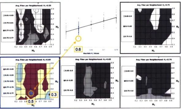
FIGURE 23: FIBER LENGTH VALUES FOR ALL HEURISTIC VALUE COMBINATIONS BY H1 GROUP... 63

FIGURE 24: H2 AND H3 AVERAGE FIBER PER NEIGHBORHOOD AREA PLOTS PER H1 GROUP ... 64

FIGURE 25: FINAL H , H 2, H 3 VALUES ... ... 65

FIGURE 26: CAPEX MODEL OVERVIEW ... ... 67

FIGURE 27: OPEX MODEL OVERVIEW ... 68

FIGURE 28: EXAMPLE MODELED POPULATIONS... ... 72

FIGURE 29: (A) BT AND FITTED MSL CDFS, (B) RESULTING PDF ESTIMATE ... 76

FIGURE 30: CORNING FTTH PON (VAUGHN, KOZISCHEK ET AL. 2004) ... 77

FIGURE 31: REFERENCE CASE, (A) CORNING AND MSL CDF ESTIMATES (B) RESULTING PDF ... 80

FIGURE 32: CONSOLIDATED CASE, (A) CORNING AND MSL CDF ESTIMATES (B) RESULTING PDF... 80

FIGURE 33: NAP SPLITTER SITES AT MIDPOINTS OF rou t - r AND r_t - Ttn FOR SINGLE RING IOF UNIFORM POPULATION DENSITY FOR A GENERIC CO ... 85

FIGURE 34: (A) K=O AND (B) K=0.5 NAP SPLITTER SITING AND FEEDER AND DISTRIBUTION FIBER FOR SINGLE RING I OF UNIFORM POPULATION CORRESPONDING TO A GENERIC CO ... ... 86

FIGURE 35: CAPEX PER SUBSCRIBER FOR (A) CORNING (VAUGHN, KOZISCHEK ET AL. 2004) AND (B) MSL FOR FOUR INITIAL BUILD VALUES AS A FUNCTION OF PENETRATION PERCENTAGE... ... 90

FIGURE 36: CAPEX PER SUBSCRIBER FOR (A) REFERENCE AND (B) CONSOLIDATED CASES WITH PARAMETERS BUILD=30%, PENETRATION=20% IN FIGURE 35(B) ... 91

FIGURE 37: CAPEX PER SUBSCRIBER COSTS VS. PENETRATION BY CATEGORY AT 30% BUILD FOR (A) REFERENCE AND (B) CONSOLIDATED SCENARIOS ... ... 92

FIGURE 38: CAPEX PER SUBSCRIBER BY INDIVIDUAL COST CATEGORY, 30% BUILD FOR (A) REFERENCE AND (B) CONSOLIDATED CASES... ... 93

FIGURE 39: EFFECTS OF LEGACY FEEDER CONDUIT ON REFERENCE AND CONSOLIDATED CASES IN FIGURE 35(B) AT 80% BUILD VS. PENETRATION ... ... 94

FIGURE 40: MSL-ESTIMATED OPEX FOR THE 30% BUILD, 20% PENETRATION REFERENCE AND CONSOLIDATED CORNING CASES IN FIGURE 36 BY (A) NETWORK ELEMENT AND (B) COST DRIVER ... 95

FIGURE 41: MSL GENERATED OPEX COMPONENTS AS A FUNCTION OF PENETRATION FOR THE 30% BUILD (A) REFERENCE AND (B) CONSOLIDATED CASES IN FIGURE 36 ... ... 96 FIGURE 42: MSL ESTIMATED OPEX DRIVER PROFILE BY NETWORK ELEMENT FOR THE (A) REFERENCE AND (B) CONSOLIDATED 30% BUILD, 20% PENETRATION CORNING CASES... ... 97

FIGURE 43: REGION IV SPATIAL POPULATION DISTRIBUTION... 102

FIGURE 44: BASE CASE CAPEX PER SUBSCRIBER FOR (A) HIGH DENSITY, AND (B) LOW DENSITY POPULATION D EM O G R A PH IC S ... 106 FIGURE 45: BASE CASE OPEX PER SUBSCRIBER FOR (A) HIGH DENSITY AND (B) LOW DENSITY POPULATION

D EM O G R A PH IC S ... ... 10 8 FIGURE 46: DISCOUNTED LIFETIME COSTS PER SUBSCRIBER AS A FUNCTION OF DISCOUNT RATE FOR THE (A) HIGH

DENSITY AND (B) LOW DENSITY REGIONS ... 110

FIGURE 47: TECHNOLOGY STRATEGY AS A FUNCTION OF PENETRATION AND DISCOUNT RATE FOR (A) HIGH DENSITY, AND (B) LOW DEN SITY REGIONS ... 111 FIGURE 48: TOTAL DISCOUNTED NETWORK COST PER SUBSCRIBER AS A FUNCTION OF PENETRATION FOR THE

HIGH-DENSITY CASE AT DISCOUNT RATE 10%, AND 100% BUILD WITH PENETRATION REGION 0.35 TO 0.7 SHOWN EXPANDED. BASE CASE PENETRATION SHOWN FOR REFERENCE ... 113 FIGURE 49: TOTAL DISCOUNTED NETWORK COST PER SUBSCRIBER AS A FUNCTION OF PENETRATION FOR THE

HIGH-DENSITY CASE AT DISCOUNT RATE 20%, AND 100% BUILD WITH PENETRATION REGION 0.45 TO 0.85 SHOWN EXPANDED. BASE CASE PENETRATION SHOWN FOR REFERENCE ... 113 FIGURE 50: TOTAL DISCOUNTED NETWORK COST PER SUBSCRIBER AS A FUNCTION OF PENETRATION FOR THE

LOW-DENSITY CASE AT DISCOUNT RATE 10%, AND 100% BUILD WITH PENETRATION REGION 0.29 TO 0.34 SHOWN EXPANDED. BASE CASE PENETRATION SHOWN FOR REFERENCE ... 115 FIGURE 51: TOTAL DISCOUNTED NETWORK COST PER SUBSCRIBER AS A FUNCTION OF PENETRATION FOR THE

LOW-DENSITY CASE AT DISCOUNT RATE 20%, AND 100% BUILD WITH PENETRATION REGION 0.3 TO 0.4 SHOWN EXPANDED. BASE CASE PENETRATION SHOWN FOR REFERENCE ... 115 FIGURE 52: LOW-DENSITY TECHNOLOGY STRATEGIES EXHIBITING LEAST TOTAL DISCOUNTED NETWORK COSTS AS A

FUNCTION OF PENETRATION AND DISCOUNT RATE FOR (A) SCENARIO 1: MB=0.95, Mc=0.9; (B) SCENARIO 2: MB= Mc= 1; AND (C) SCENARIO 3: MB= 1.05, Mc= 1.1 ... 118 FIGURE 53: LOW-DENSITY, LOW DATA-DEMAND (A) CAPEX PER SUBSCRIBER VS. PENETRATION WITH CROSSOVER

EMPHASIZED, AND (B) DISCOUNTED OPEX PER SUBSCRIBER VS. BOTH PENETRATION AND DISCOUNT RATE FOR S C EN A R IO 1 ... ... 12 0 FIGURE 54: LOW-DENSITY TOTAL DISCOUNTED COST PER SUBSCRIBER AS A FUNCTION OF PENETRATION RATE FOR

DISCOUNT RATE 7% WITH CROSSOVERS EMPHASIZED, SCENARIO 1: MB=0.95, Mc=0.9 ... 120 FIGURE 55: HIGH-DENSITY TECHNOLOGY STRATEGIES EXHIBITING LEAST TOTAL DISCOUNTED NETWORK COSTS AS A

FUNCTION OF PENETRATION AND DISCOUNT RATE FOR (A) SCENARIO 1: MB=0.95, Mc=0.9; (B) SCENARIO 2: MB= MC=l; AND (C) SCENARIO 3: MB=1.05, Mc= ... 123 FIGURE 56: HIGH-DENSITY, HIGH-DATA DEMAND (A) CAPEX PER SUBSCRIBER VS. PENETRATION WITH CROSSOVER

EMPHASIZED, AND (B) DISCOUNTED OPEX PER SUBSCRIBER VS. BOTH PENETRATION AND DISCOUNT RATE FOR

TABLE OF TABLES

TABLE 1: FIBER PLANT LINK DESCRIPTIONS ... ... ... 13

TABLE 2: ARCHITECTURE IMPLEMENTATION STRATEGIES BY GPON TECHNOLOGY CHOICE ... 17

TABLE 3: PARAMETERS AND VALUES OF f p (r) IN FIGURE 3 ... ... 27

TABLE 4: NEIGHBORHOOD DIMENSIONS AND LOCATION DENSITY AS A FUNCTION OF DISTANCE R... 34

TABLE 5: DR, Np=1(r), AND p" VALUES FOR POPULATION P=1 IN FIGURE 3 ... 34

TABLE 6: HOUSEHOLD SIZE CATEGORIES AND VALUES USED IN FIGURE 3 ... 36

TABLE 7: SPECIFIC g ( ) VALUES FOR POPULATIONS IN FIGURE 3 ... 36

TABLE 8: SUBSCRIBER SIZE BINS AND POPULATION FRACTIONS IN FIGURE 3 ... 37

TABLE 9: hP41 (r) VALUES FOR POPULATION P=I IN FIGURE 3... 38

TABLE 10: hp={2,3}(r) PROBABILITIES FOR POPULATIONS P=2 & 3 IN FIGURE 3 ... 39

TABLE 11: HOUSEHOLD PER LOCATION PROFILE FOR POPULATION P=1 IN FIGURE 3 ... 40

TABLE 12: SERVICE TIERS AND SERVICES FOR POPULATIONS IN FIGURE 3 ... 41

TABLE 13: kp (prt) VALUES FOR MODELED POPULATIONS IN FIGURE 3 ... ... 41

TABLE 14: p=(1,2,31 (r) VALUES FOR POPULATIONS P=1;2;3 IN FIGURE 3 ... 42

T 1 t=,2,3}) TABLE 15: CONDITIONAL DATA TIER PROBABILITIES AS A FUNCTION OF DISTANCE R ... 42

TABLE 16: TECHNOLOGICAL CONSTRAINTS... 43

TABLE 17: LINK TOPOLOGIES MODELED ... ... 46

TABLE 18: INSTALLED FIBER LENGTH AS A FUNCTION OF R ... ... 49

TABLE 19: DISTANCE CONSTRAINT VALUES BY DISTANCE REGION... ... 52

TABLE 20: HEURISTIC CALIBRATION POPULATION PARAMETER VALUES ... ... 60

TABLE 21: HEURISTIC CALIBRATION TECHNOLOGY CHOICE... 61

TABLE 22: HEURISTIC PARAMETER VALUES MODELED ... 62

TABLE 23: FINAL HEURISTIC VALUES ... 64

TABLE 24: COST MODEL NETWORK ELEMENT CATEGORIES AND COMPONENTS ... 66

TABLE 25: OPEX COST CATEGORIES AND COMPONENTS... ... 67

TABLE 26: SAMPLE MUNICIPALITY TECHNOLOGY AND POPULATION PARAMETER VALUES (KERSEY 2006)... 68

TABLE 27: POPULATION DEMOGRAPHICS (KERSEY 2006) ... 69

TABLE 28: DATA DEMAND DEMOGRAPHICS (KERSEY 2006) ... 69

TABLE 29: OUTAGE STATISTICS (KERSEY 2006) ... 69

TABLE 30: NETWORK LABOR REQUIREMENTS (KERSEY 2006)... 70

TABLE 3 1: AVERAGE NETWORK OPEX VALUES (KERSEY 2006) ... 70

TABLE 32: PARAMETER VALUES MODELED ... ... 72

TABLE 33: TEST RESULTS FOR a=5KMAND =10OKMSCENARIOS... 73

TABLE 34: TEST RESULTS FOR a=15KMAND a =20KMSCENARIOS... 73

TABLE 35: SUMMARY STATISTICS, INTERNAL CONSISTENCY TEST... ... 74

TABLE 36: BT EXCHANGE PARAMETERS ... ... 75

TABLE 37: BT EXCHANGE POPULATION CHARACTERISTICS ... 75

TABLE 38: MSL AND BT NETWORK METRIC COMPARISON ... ... 76

TABLE 39: CORNING FIBER LENGTH CONSTRAINTS AND PARAMETER VALUES (VAUGHN, KOZISCHEK ET AL. 2004) ...7 7 TABLE 40: HOUSEHOLDS BY CENTRAL OFFICE (VAUGHN, KOZISCHEK ET AL. 2004) ... 78

TABLE 41: HOUSEHOLD DISTRIBUTIONS, REFERENCE CASE (VAUGHN, KOZISCHEK ET AL. 2004)... 78

TABLE 42: HOUSEHOLD DISTRIBUTIONS, CONSOLIDATED CASE (VAUGHN, KOZISCHEK ET AL. 2004)... 79

TABLE 43: CORNING STUDY SPLITTER RATIOS (VAUGHN, KOZISCHEK ET AL. 2004)... 81

TABLE 44: TOTAL ESTIMATED SPLITTERS REQUIRED PER CO BY DISTANCE FROM CO ... 82

TABLE 46: LCP SPLITTER SITES AND FEEDER FIBER LENGTHS PER DISTANCE REGION I: COA REFERENCE CASE

... 84

TABLE 47: COMPLETE NAP AND INSTALLED FIBER DISTANCES FOR COA REFERENCE CASE ... 88

TABLE 48: ESTIMATED CORNING MINIMUM AND MAXIMUM TOTAL INSTALLED FIBER LENGTHS AND MSL NETWORK MODEL FIBER LENGTH RESULTS FOR ALL COs... 88

TABLE 49: TECHNOLOGY CHOICES AND IMPLEMENTATION STRATEGIES MODELED ... 99

TABLE 50: POPULATION DEMOGRAPHIC SPACE ... 100

TABLE 51: BASE CASE POPULATION PARAMETER VALUES ... 101

TABLE 52: REGION IV CUSTOMER LOCATION DATA ... 102

TABLE 53: REGION IV HOUSEHOLD SIZE CATEGORIES AND VALUES ... 103

TABLE 54: REGION IV HOUSEHOLD SIZE DISTRIBUTION VALUES ... 103

TABLE 55: REGION IV TOTAL HOUSEHOLDS PER POPULATION ... 103

TABLE 56: REGION IV SPATIAL HOUSEHOLD DISTRIBUTION... 103

TABLE 57: REGION IV HOUSEHOLDS PER LOCATION CONDITIONAL PROBABILITY PROFILE BY DISTANCE REGION, PO PU LA TIO N S 1 & 2 ... ... 104

TABLE 58: REGION IV HOUSEHOLDS PER LOCATION CONDITIONAL PROBABILITY PROFILE BY DISTANCE REGION, POPULATIONS 3 & 4 ... 104

TABLE 59: REGION IV DATA SERVICE TIERS... 104

TABLE 60: REGION IV SERVICE TIER POPULATION PERCENTAGES ... ... 104

TABLE 61: REGION IV DATA TIER SPATIAL DISTRIBUTION ... 105

TABLE 62: REGION IV SPATIAL DISTRIBUTION OF DATA TIERS, POPULATIONS 1 & 2 ... 105

TABLE 63: REGION IV SPATIAL DISTRIBUTION OF DATA TIERS, POPULATIONS 3 & 4 ... 105

TABLE 64: CAPEX UNCERTAINTY SCENARIOS CONSIDERED FOR EACH POPULATION BY TECHNOLOGY ... 117

TABLE 65: VARIANCE, M, AND MULTIPLIER, M,, VALUES MODELED FOR THE LOW-DENSITY, LOW-DATA DEMAND CASE ... 119

1 Introduction

As the demand for broadband communications continues to expand and the technologies for satisfying that demand continue to evolve, access network operators are confronted with a host of challenging questions surrounding technology choice and network deployment. Ultimately, any service provider is trying to identify a technology choice that allows them to both profitably serve their subscribers today and adapt to future market changes. Given the range of contributing issues and the rapidly evolving state of technology, it is very difficult for one firm to answer such questions alone. Currently, standards bodies are exploring a multitude of technology choices for future optical broadband network networks. Often, carriers find themselves necessarily myopic when considering which network architecture to choose. Legacy-centrism results in the construction of modeling tools which focus on a specific network design, and often, a particular architectural winner is chosen and focused on early, further obscuring the benefits a complete, general architectural comparison might provide. Understanding the cost tradeoffs resulting from technology choice free from the constraints of either existing networks, or an individual carrier's preferred architecture, requires a generalized approach characterizing the relative cost tradeoffs

for a range of population/demand demographics. Next-generation gigabit passive optical network (GPON) architectures will offer not only higher bandwidths enabling more products and services, but also better quality of service, enabling more efficient and reliable networks, thereby increasing subscriber satisfaction and retention rates. These benefits will require significant upfront capital investments however, which will both "lock in" the resulting technology through standardization and component economies of scale and learning, and act as a barrier to future implementation of different technology choices. Given the decades long life cycles associated with these networks, it is important to characterize both the long-term cost implications of near-term technology choice decisions, and the long near-term benefits of investing in longer-near-term technology solutions. These issues suggest several questions for carriers and standards bodies to consider before selecting a technology:

1. How does a long-term view of network costs including operational expenditures (OpEx) impact initial technology choice decisions?

2. What are the cost implications and tradeoffs resulting from implementing GPON technologies available in the near future, versus waiting to deploy future technologies whose costs are unknown?

3. How should a particular technology choice be implemented to reduce total network costs?

4. How do population and data demand demographics affect technology and architecture choice?

5. How do legacy network, subscriber service penetration and discount rate impact

technology choice decisions?

This work examines implementation strategies for three different GPON technology choices. These technologies were selected not only because they differ in technical specifications, but also because they present carriers with three different implementation timeframes: from technologies currently being deployed for which costs are known; to technologies which have been demonstrated in small-scale mockups but are not ready for deployment and for which costs are more uncertain; to long-term solutions with the potential to significantly reduce expensive network components, but for which cost data is either unknown or not yet available.

This thesis provides a suite of three integrated modeling tools, providing decision makers with a descriptive, rather than normative, toolset, to characterize and compare the relative lifetime network costs of each technology choice for multiple population demographics and under different technology implementation strategies. The first tool is a statistics-based population generator which parameterizes populations with different characteristics. Next, a network-modeling tool utilizes this population data and technology-specific architecture parameters to dimension large-scale network architectures. Finally, comprehensive cost models utilize cost and statistical component failure data from both manufacturers and real-world deployments to characterize how network costs change in response to technology choice decisions for a given population.

1.1

Passive Optical Network Overview

In their simplest incarnation, passive optical networks (PONs) consist of four main elements:

metro access nodes, (MANs), which aggregate and route data for hundreds of thousands of

subscribers between cities; central offices, (COs) which house the transmission and receiver equipment required to provide service to tens of thousands of customers; splitters, which enable a single transmission line from the CO to serve tens of subscribers; and the customer premise

service to individual subscribers. Linking these network components together are fiber optic cable bundles of various sizes collectively known as the fiber plant. Collectively, these elements comprise the main network sections: the backhaul network, consisting of all fiber bundles and equipment connecting MANs to COs and MANs to MANs, and the local access network, (LAN) containing the equipment and fiber links required to connect subscribers to COs and connecting COs. Figure 1 illustrates the basic "fiber-to-the-home" network topology for a architecture with two back-to-back or cascaded splitter stages, each enabling a single line from the CO to be split

four ways. As a result, each transmission line can reach up to sixteen subscriber locations.

Local Access Network

Inter-city

(1)

(5)

I

Backhaul (3) (4)

Network

---

-Metro Access C ral Splitter Fber Customer

Node (MAN) Offc Sa Link ID Lo o Figure 1: Basic GPON network architecture

In the literature, fiber links are classified in one of four categories depending on which network

elements they connect. Backhaul fiber connects the MAN and COs and CO to CO; feeder fiber connects COs to the first splitter stage; distribution fiber links splitter stages; and drop fiber connects the final splitter stage to the subscriber, (in "fiber-to-the-home" networks) or to curbside aggregation points, which then are connected to the subscriber via copper wires, (in "fiber-to-the-curb networks"). This work focuses on the former. Table 1 classifies the relevant fiber link lengths shown in Figure 1.

Fiber Link ID Fiber Link Description Fiber Link

1 MAN to CO Backhaul

2 CO to CO Backhaul

3 CO to splitter Feeder

4 Splitter to splitter Distribution

5 Splitter to subscriber Drop

These networks have traditionally been called "passive" because none of the network equipment between the CO and subscriber, (splitters and fiber) requires a power source. However, recent technologies which introduce signal-boosting amplifiers in this portion of the network, (some of which will be modeled in this thesis) are also classified as passive optical networks.

In general, the maximum times a signal may be split and the total distance from the transmission equipment in the CO to a subscriber is determined by the network-specific power budget. This power budget is defined by subtracting the receiver sensitivity of the customer premise equipment, Rx, (a measure of the subscriber receiver's ability to detect incoming signal power) and desired safety margin, SM, (a built in buffer to compensate for signal power fluctuation) from the signal transmission power (Tx) (in milli-decibels1, dBm). If the technology choice uses signal-boosting amplifiers, the signal power gain, PAmp, is then added, and any related power losses due to amplifier insertion, LAmp, are subtracted. Signal loss due to signal splitting, Lspitter,

scales as a loss constant, c, multiplied by the base-two logarithm of the number of splitter ports. For example, a 1:4 way splitter will result in a signal power loss given by,

Lspter = clog2(4)= 2.c, while a 1:16 way splitter result in a loss of Lspitter = clog2(16) = 4.c.

As a result, a network with a given power budget can either have a longer reach at a lower splitter port count or have a shorter reach but a higher splitter ports count. This tradeoff suggests that multiple splitter ratio/network reach implementation strategies are possible for a given technology choice2.

To define network reach, (in kin) the remaining power budget is divided by the power loss per fiber kilometer, (LFiber, an intrinsic fiber property). Symbolically, the reach determination relationship is given by:

Tx - R -SM PAmp - LAmp - LSplitters dBm =

R

LFiber d B/km

All subscribers served by a single feeder fiber must share not only the signal transmission power of a given optical line, but also the available data rate. The maximum transmission rate for a given optical line terminal (OLT) port, (the laser and modulator combination creating and shaping the signal) and the method for combining multiple subscriber data onto a single line, (the

1 A logarithmic ratio which measures signal power magnitude relative to a reference level of 1 milliwatt, defined as dBm = 10loglo(P1/Po), where P1 is the transmitter signal power and Po = 1 milliwatt.

"multiplexing" strategy) are specific to technology choice. All technologies modeled in this work utilize Statistical Time Division Multiplexing, (STDM) to allocate subscriber bandwidth. STDM divides a single data stream into discrete "packets" containing both an individual subscriber's data, and the corresponding optical network terminal (OLT) address. Packets are then assigned dynamically on an as needed basis. This dynamic bandwidth allocation enables both "burst-mode" transmission, whereby an individual subscriber may be assigned large fractions of the total data stream, and "statistical gain," which effectively reduces the data burden of each subscriber under the assumption that all subscribers will not simultaneously request their maximum subscription service3.

1.2 Overview of Technology Choices

Modeled

Three fiber-to-the-home GPON technologies were selected which represent a spectrum of current and future networks. Because power budget allocation enables multiple implementation strategies for each technology (see above discussion), several such strategies were modeled.

A. "Standard" GPON. This is the least complex GPON technology choice, in that all components outside the central transmission office are completely "passive": using only chromatic splitters and without signal amplification. As a result, this choice exhibits the smallest total signal power budget, limiting both split ratio (typically 1x32 way total splitter ports) and CO to subscriber network reach (typically 20-25km). Because this technology employs many components already in production, and is governed by an established standard, 2003 IEEE ITU-T G.984.1 GPON, it represents the nearest-term GPON solution. Therefore, it is used as a benchmark against which to value the other technologies considered.

B. Amplified GPON. This technology utilizes remote-powered semiconductor optical amplifiers (SOAs) outside the central office to increase the available power budget, enabling either longer reach (up to the theoretical 60km distance limit of the GPON standard (Lin 2006)) or higher split (up to lx256 total port count) architectures. The increase in reach and/or customers per transmission line due to amplification enables multiple reach/split ratio architecture combinations, some of which may reduce network

3 One drawback to this method is that simultaneous maximum data demands may reduce the data available for all subscribers to levels below the agreed upon subscription rates

CapEx and OpEx by reducing the number of central offices required to service the coverage region. Early working models of this technology have been demonstrated (Nesset, Payne et al. 2006), and the additional network elements required have been thoroughly researched and are beginning to be manufactured, albeit not at the scale required to bring cost on par with the "standard GPON" components described above. Therefore, this technology choice represents our "mid-term" future solution.

C. Long-Range GPON utilizes high-gain erbium-doped fiber amplifiers (EDFAs) to significantly extend both the reach (up to 100km) and split ratio (up to 1x1024 total ports). The extended reach enables the elimination of central offices completely, instead connecting all customers directly to the metro access node, (MAN) which traditionally serves as a gateway between local access networks (LANs) for the other technologies (connecting city to city for example). This results in the location of all transmission equipment at MAN locations, and eliminates the need for backhaul-related equipment which would otherwise be required to connect central offices in the LAN to the MANs servicing the coverage region. This technology is currently the furthest away for implementation, and is not currently covered by the existing GPON standard. Additionally, the component costs for the additional network elements required to enable this technology are currently unknown. Therefore, this choice is modeled as a "long-term" future GPON solution.

It is important to note that the technologies selected for this analysis do not constitute an exhaustive set of strategies under consideration, but are intended to be representative of the spectrum of Statistical Time Division Multiplexed (STDM) options currently being explored by carriers. Table 2 provides an overview of the implementation strategies modeled for each technology choice, for example, "Al" corresponds to the first implementation strategy for technology choice "A" ("standard" GPON). The assumed advantages and disadvantages of each strategy, along with more in depth technical parameters will be provided in Chapter 10.

Implementation Al A2 B1 B2 B3 C1 C2 Strategy

Downstream 2.5 Gbps

Data Rate

Multiplexing Statistical Time Division Multiplexing (STDM)

Strategy

Splitter Centralized _Cascaded

Configuration

Total Splitter 1x32 1x32 lx128 1x256 lx512 lx512 lx1024

Port Count

Total Network 25 25 60 53 46 100 88

Reach (km)

Amplification N/A N/A SOA SOA SOA EDFA EDFA

Strategy

Table 2: Architecture implementation strategies by GPON technology choice

1.3 Thesis Outline

Chapter 2 presents an overview of current network modeling approaches, and discusses the gaps the thesis intends to address. Chapter 3 presents the expected research contributions, and Chapter 4 provides a brief overview of the modeling methodology used to achieve these goals. Chapter 5 introduces the population generator, which characterizes important population attributes based on input probability distributions. Chapter 6 describes the network model including inputs and the heuristic-based modeling algorithms used to dimension a virtual network, and Chapter 7 focuses on the heuristic calibration process and sensitivity analysis to the final heuristic value set. Chapter 8 explains both the CapEx and OpEx cost models and component cost data collection, while Chapter 9 performs benchmarking and validation exercises for the network and cost models, and then discusses the methodology capabilities and limitations. Chapter 10 defines the populations, architecture parameter values, methodologies, results, analyses and result sensitivities for the cases modeled. Finally, Chapter 11 provides the analysis conclusions and recommendations to firms, and Chapter 1 suggests future work.

2 Current Modeling Approaches

Modeling comparisons of network costs due to technology choices requires three things: a way to fully characterize the important aspects of a subscriber population, a network dimensioning tool which accurately reflects how fiber plant and component requirements change as a function

of technology choice and these population characteristics, and cost models which accurately characterize network lifetime costs, both capital and operational expenses, corresponding to each dimensioned network. This chapter examines different existing approaches to these three requirements, identifies gaps, and discusses how the MSL modeling approach addresses these gaps.

2.1

Network Modeling Approaches

Network design models must perform several functions, including siting central offices (COs), splitters, and amplifiers, and defining the fiber route topology connecting all these network components to both each other and subscribers. Additionally, many factors contribute to shape each function's output, including topological/geographic constraints of the connected region; existing/legacy facilities and/or fiber routes; and component/fiber performance, availability, cost, and capacity.

The literature reveals two classes of approaches carriers use when dimensioning optical broadband networks. The first, which we label "bottom-up," incorporates population and data demand information on every potential subscriber in the coverage region and problem-specific constraints to dimension cost-minimizing networks through optimization. The second approach, which we label "top-down," utilizes engineering rules of thumb developed over time in the telecommunications industry to dimension larger populations or specific population sub-types, (a

square grid of urban city blocks for example).

2.1.1 Bottom-Up Optimization Approaches

Much work has been done to address the difficult optimization problems required to minimize network costs subject to these many constraints. Telecommunications network design problems involve multiple layers to be optimized simultaneously. For example, the physical layer concerns the geographic network topology, while the traffic layer concerns the flow of information through the physical infrastructure and the corresponding link data capacity required to meet customer demand at all times. These complex optimization problems all attempt to minimize (or potentially maximize depending on criteria) an objective function, typically total network costs, subject to constraints on link capacity, while connecting all transmission data sources to subscriber data sinks in the context of a specific technology choice. Problems of this type have two "flavors". The first involves siting data concentrators, (central offices and splitter sites),

given subscriber locations, subject to satisfying data demands, (see (Gourdin, Labbe et al. 2002). These concentrator location or capacitatedfacility location problems often arise in other areas such as transportation, and produce tree topologies. These problems are often modeled using mixed integer programming models and various heuristic-based constraint relaxation techniques for both tree network (concentrator to subscriber point to point connections) (Balakrishnan, Magnanti et al. 1991; Ahuja, Magnanti et al. 1993; Balakrishnan, Magnanti et al. 1995; Daskin 1995; Klincewicz 1998), and ring structures, (Klincewicz 1998; Ramaswami and Sivarajan 2002). The second problem variety assumes that concentrator and subscriber locations are known. The Multi-capacity flow problem takes these locations, data sources (nodes) and the rules about the allowable connections between them (links), and routes traffic from individual sinks to concentrator points and vice-versa. Such problems have also been modeled extensively using graph theoretic, and linear programming and multiple other approaches for both tree networks, (see (Boorstyn and Frank 1977; Balakrishnan, Magnanti et al. 1991; Gavish 1992; Ahuja, Magnanti et al. 1993) and ring network design, (LeBlanc, Park et al. 1996; Sanso and Soriano 1999; Sridhar, Park et al. 2000). See (Nagy and Salhi 2007) for a thorough survey of algorithmic methods and approaches throughout a variety of fields.

Often, problems of this type require decomposition into different components which are then individually solved to optimality when possible, or through heuristic approximation and constraint relaxation (Carpenter and Luss 2006). While exact solutions exist for relatively small problems, (on the order of 50-100 nodes, see (Gabral, Knippel et al. 1999; Minoux 2001), to optimize over the potentially millions of customers, multiple central offices, and hundreds of splitter sites required to serve a large coverage region becomes computationally intractable, as computational time grows rapidly as the number of nodes and edge possibilities increases4, (Gabral, Knippel et al. 1999; Melkote and Daskin 2001; Randazzo and Luna 2001; Klose and Gortz 2006; Lee, Kim et al. 2006; Prins, Prodhin et al. 2007; Li, Chu et al. 2009).

2.1.2 Top-Down Engineering-Rule-Based Approaches

In contrast to the mathematical optimization modeling approaches described above, these methods utilize the experience of network designers and widely recognized engineering rules of thumb to examine the relative cost impacts of technology choice in networks serving small

4In general, these problems are "NP-hard," defined a class of problems for which no solution can be found using an algorithm in polynomial time. As a result, the problem scales exponentially with the number of nodes.

populations or specific population types. These models often characterize populations using information drawn from experience with previous network deployments or actual populations currently serviced. For example, a 2003 Bell Labs study (Weldon and Zane 2003) modeled several technology choices serving a small population with uniform population density occupying a square grid resembling a cluster of urban city blocks. This grid structure enables the derivation of simple fiber-routing rules, which are then used to dimension the fiber to the home network topology. The costs of different technologies are then compared for this topology at different penetration (subscriber uptake) levels. By contrast, a 2004 Coming study, (Vaughn, Kozischek et al. 2004) models the cost implications of technology choice and implementation strategies for a network serving up to 70, 000 subscribers. This model breaks down the population into discrete categories by blocks of distance from three pre-located central offices. All subscribers in each category are then assigned a characteristic average fiber length, and these lengths are summed to arrive at an estimate of the total fiber required to provide data services. For example, all customers at a distance of three kilometers or less from a central office are assigned a feeder fiber length of 0.59km. Different penetration rates are then modeled by adding or subtracting these average values and the corresponding customer premise equipment.

2.1.3 Network Modeling Approach Comparison and Gap Analysis

The "bottom-up" optimization and "top-down" engineering rule of thumb approaches bound the spectrum of network dimensioning tools: the former requires extensive collection of often proprietary data and computational power, but potentially provides mathematically optimal topologies for small populations, while the latter takes advantage of engineering expertise and experience and requires relatively simple computational tools, but may miss important details impacting network design by limiting analysis to population subtypes and assigning coarse fiber plant characteristics to large fractions of the population.

A method incorporating the optimization-focus of the bottom up approach with the computational tractability of the top-down approach would enable characterization of how technology choice and population demographics drive relative topology changes between networks. Instead of exhaustively optimizing a single network and/or technology, this method could enable large populations to be modeled for multiple technologies. Such a model could capitalize on the strengths of both optimization and engineering-rules based approaches, but

avoid the computational complexity of the former while more accurately characterizing how population and technology attributes drive network topology than the latter.

2.2 Population Characterization Approaches

Population demographics can impact network cost at least as much as technology choice (Sirbu and Banerjee 2005). Therefore, it is important to accurately characterize these relationships. For example, intuitively high subscriber population and data demand densities translates into large quantities of central offices, transmission optical line terminals (OLTs), splitter sites, and amplifiers than those required to serve sparser regions and/or those with smaller data demands. Not as immediately obvious however is the impact on fiber length of changes in population density. For example, in urban areas, the fiber length from the curb to a subscriber location is significantly less than the same link length required to span a front yard in a suburban neighborhood, or the often-significant acreage from road to urban homes. Reinforcing this effect is that a single curb to location trenched fiber can often reach multiple subscribers sharing apartment buildings in dense urban areas, while, in suburban areas there are many more single-family homes, each of which requires an individual fiber. Add to this the fact that each subscriber at a given location can require different data service tiers, potentially resulting in fewer customers served per splitter, as the maximum transmission rate per individual service line is limited. For large coverage regions with hundreds of thousands or millions of homes passed, these differences can translate into thousands of kilometers of installed fiber length-and millions of dollars in capital and operational expenses. Therefore, it is important to accurately characterize how population density, household density, and data demand density characteristics change throughout the subscriber population.

There are two population-modeling approaches in the telecommunications literature, corresponding to the two network modeling approaches outlined above: explicitly modeling every home in the coverage region, and assigning average or uniform values to population characteristics. Inherent in the "bottom-up" approach to network modeling is an assumption that every subscriber location in known. These "nodes" form the basis of graph-theoretic approaches to the multi-capacity flow problems, (Balakrishnan, Magnanti et al. 1991; Ahuja, Magnanti et al. 1993; Balakrishnan, Magnanti et al. 1995; Daskin 1995; Klincewicz 1998). and serve as the data sinks requiring splitter and central office siting in concentrator location problems (Boorstyn and

Frank 1977; Balakrishnan, Magnanti et al. 1991; Gavish 1992; Ahuja, Magnanti et al. 1993) (LeBlanc, Park et al. 1996; Sanso and Soriano 1999; Sridhar, Park et al. 2000) (Nagy and Salhi 2007). This makes sense, as optimization focuses on meeting the demands of a specific population given a technology choice. By contrast the "top-down" dimensioning approaches relax the constraint of explicitly characterizing every subscriber in favor of coarser metrics such as average or uniform densities, (Weldon and Zane 2003; Vaughn, Kozischek et al. 2004; Joao 2007). This also makes sense, given that these studies focus on characterizing the cost

implications of different technology choices given a simple population or population subtype.

2.2.1 Population Characterization Gap Analysis

While explicitly modeling every customer location in the coverage region may ensure complete population characterization, it introduces three complications: (a) it is data intensive, requiring the physical location, household size, and data demands of every subscriber; (b) these large data sets require computationally complex optimization algorithms whose solution time scales with problem size; and (c) it is difficult to generalize, as the resulting resource-intensive algorithm "overfits" to satisfy the specified population. Conversely, coarse characterizations of population attributes, while enabling the relatively computationally simple dimensioning algorithms to dimension, may overlook important subtle yet important cost drivers. Between these two approaches exists an opportunity for a method which balances the detail required to characterize how these important attributes change across a population, against the abstraction required to easily model multiple technologies. Additionally, characterizing populations free from proprietary carrier data may help facilitate more detailed discussion about technology choice.

2.3 Cost

Modeling

Approaches

Characterizing lifetime network costs requires examining not only large capital investments, but also recurring operational costs. Traditionally, cost models have focused on the CapEx associated with technology choice, (Weldon and Zane 2003; Vaughn, Kozischek et al. 2004; Joao 2007). However, this approach obscures any potential OpEx savings associated with a particular technology choice. Often, when OpEx is considered, it is treated as a simple mark-up on network CapEx (Konrad 2007). This approach suggests that multiple technologies with similar CapEx should be considered on equal footing from an implementation standpoint; however, studies have shown that fiber to the home optical networks can provide substantial

OpEx savings over existing copper networks (Halpern, Garceau et al. 2004; Wagner, Igel et al. 2006). As a result, recent studies have begun to more thoroughly examine network OpEx and classify the important cost drivers (Verbrugge, Pasqualini et al. 2005). These studies either try to find ways to optimize the repair and maintenance infrastructure of existing networks, (Casier, Verbrugge et al. 2007) or focus on characterizing service-based OpEx, (Pasqualini, Kirstadter et al. 2005; Konrad 2007; Machuca, Moe et al. 2007; PrieB and Jacobs 2007; Vukovic 2007; Vusirikala and Melle 2007). Broadly, these methods comprise a set of "bottom-up" approaches, (Konrad 2007; Prief and Jacobs 2007) which seek to characterize OpEx as the sum of network elements necessary to meet a customer demand scenario, rather than "top-down" methods which assign total network costs to network components.

2.3.1 Cost Modeling Gap Analysis

While many studies have done an excellent job of characterizing network CapEx, few studies have integrated CapEx with detailed network OpEx to compare lifetime network costs across technologies and/or population demand scenarios. For example, top-down methods rely on proprietary cost information for a specific, deployed network, while bottom-up approaches allocate costs to products and services for existing or mathematically optimized future networks. As a result, both methods limit the generalizability of results, the former through lack of transparency and access to data, and the latter via over-optimization or undervaluation of dynamic OpEx drivers such as maintenance (Konrad 2007; Prie3 and Jacobs 2007).

3 Expected Contributions

This thesis addresses the role of OpEx in initial technology decisions for several FTTx GPON technologies, each with multiple possible implementation strategies. The methodology employed utilizes three, novel models integrated into a single methodological modeling framework: a population generator and characterization tool, a heuristic-based network dimensioning model, and a capital and statistical operational cost model. This method is then used to gain case-specific insights into parameters which drive OpEx, including population demographics and cost uncertainty of future technologies.

The first model component characterizes subscriber populations in multiple dimensions which constrain and alter network topology: location density, household density, and data demand

density. This ability to specify detailed population characteristics for multiple populations enables exploration of how these characteristics affect network costs, and the ability to model multiple populations and/or large geographic regions. The model samples from three, independent input population distributions, (one for each density parameter) and then uses conditional probabilities to determine how these densities change as a function of distance from the population center. Sampling reduces the data required to characterize a population while maintaining important population attributes. Additionally, modeled populations provide generic, and therefore generalizable, characteristics free from proprietary data constraints.

The second model component utilizes this data set and three heuristics to dimension a virtual network. Because fiber installation is the primary driver for network CapEx, (Wagner, Igel et al. 2006) and fiber-related outages drive OpEx labor costs, (Rand-Nash, Roth et al. 2007) the model emphasizes fiber minimization via maximum co-location. Rather than seeking a mathematically optimized solution, the model utilizes constraints based on the three population parameters defined above to determine how technology choices affect relative network topology via fiber plant and central office siting. Additionally, because sampling reduces the data intensity needed to characterize the population, the network model requires less computational power, enabling rapid modeling of multiple technology choices.

Finally, the cost models model incorporate real-world installation, failure and operations data with industry component cost and failure data to characterize how technology choice and population demographics impact lifetime network costs. By gathering cost data from multiple sources throughout the telecommunications industry, the model is able to escape proprietary point cost estimates, thereby increasing transparency and generalizeability, and assign a complete set recurring costs including scheduled maintenance and normal operations costs and probabilistic repair and replacement costs to the dimensioned network.

4 Methodological Overview

The MIT Materials Systems Laboratory (MSL) Population Generator, Network Design and Cost Models determine network lifecycle costs, and how these costs change in response to changes in assumed technological (e.g. transmitter power), demand (e.g. subscriber distribution), and operational characteristics (e.g. coverage area). Figure 1 provides an overview of the modeling approach.

Network Model Inputs Fiber Plant Siting Network Design Model

Figure 2: Modeling Overview

The demand demographic, technological characteristics, and operating context comprise the initial set of input parameters, thereby constraining the solution space of possible network designs. The population generator characterizes the subscriber demographics. The design model then dimensions a virtual network, defines the necessary hardware quantities, and populates the network with specific, user specified hardware/component choices. Finally, the network cost

models map initial capital investments and recurring operational costs corresponding to each

resulting network.

5

MSL Population Characterization

The MSL population model attempts to attain the balance of abstraction and detail which captures the important relationships between population characteristics and network topology while using statistics and sampling to reduce data requirements and the resulting computational burdens. The model characterizes three important population attributes, using three, independent and user defined probability distributions which together form the set of demand demographics for each population. The first attribute, population density, is determined by sampling from an input probability distribution. The distribution parameters then determine how this density changes as a function of distance from the population center. The reduced data intensity enabled by population sampling, while smaller than individually characterizing every subscriber, is still quite large by optimization standards, (see §2.1 for a discussion of this issue). Therefore, the model focuses on simplifying the dimensioning process by breaking the continuous coverage region into discrete grids. The second characteristic, household size density, is determined by first defining the types of household/business sizes available, and then determining the percentages of the population with each size, and how these household sizes are distributed as a

Network Cost Models

function of distance from the population center. Similarly, the final attribute, data demand

density, is characterized by first defining the quantity and data rates of individual service tiers to

be offered, and then determining the fraction of the total population subscribing to each tier, and how this tier density is distributed throughout the population.

5.1

Population Density

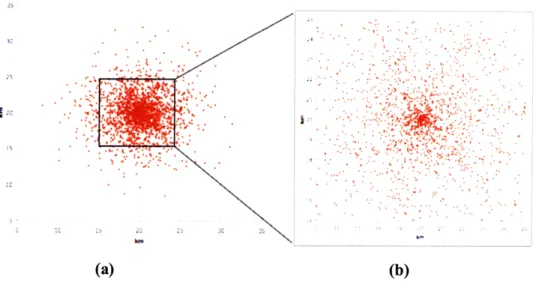
The first distribution utilizes the random variable, F, the distance from the distribution center to a subscriber location, with probability density function (pdf), frP(r), to site customer locations for each population, p. As an example, consider Figure 3, which depicts a coverage region with three population centers, (p = 1,2,3) all normally distributed but with differing standard deviations (which serve to either spread or cluster each distribution). In this specific example the standard deviations are small, on the order of 3-4 km, resulting in tight distributions (small cities). All parameter values describing each distribution, including the mean (which determines where the center of the distribution is geographically), and standard deviation are user-defined. The total coverage region shown is 100x100 km2 .

100 Sp =2 40 p =1 30 0 10 20 30 40 50 60 70 s0 90 100 n

Figure 3: Sample 100km2 coverage region with three population distributions Each colored "dot" in Figure 3 does not represent a single subscriber location, but rather a

is a user-defined input parameter5, as is the total locations per population /p. Together, these two parameters define the locations per neighborhood for each population, i" .Table 3 presents the three fP (r) related parameters and values used in Figure 3.

Parameter Definition Value used in Figure 3

P Total populations 3

p Individual population ID 1; 2; 3

T p, Type, mean and variance: population p N(0,9); N(0,16); N(0,16)

/P Locations per population 24k; 48k; 72k

dp Total neighborhoods per population 2,000; 4,000; 4,000

/d Locations per neighborhood for population p 12; 12; 24

Table 3: Parameters and values of frP(r) in Figure 3

5.2 Population Density Modeling

Because the number of subscribers (nodes in the optimization literature, see §2.1) directly relates to the computational resources required to dimension the network, the MSL population model attempts to limit these points by overlaying a search grid onto the coverage region. The grid structure, the size each cell and the total number of cells, defines the level of detail the model can resolve. For example, Figure 4 depicts a square grid overlaid on (a) the entire population and (b) a population subset ofp=l in Figure 3. The grid points are uniformly spaced one kilometer apart in both the horizontal, ("x") and vertical, ("y") directions, resulting in an individual grid point

resolution of I km2

P

5 dp 10,000

,.* " .

..- . :V;

(a) (b)

Figure 4: Square grid cells of area 1 km2 _{superimposed onp=l in Figure 3}

As Figure 4(a)(b) illustrates, this grid structure results in a significant number of empty grids in sparse regions, and grids containing many neighborhoods in dense regions. The former results in an inefficient search, as computational resources are spent checking empty grids, while the latter results in poor resolution in much of the region, potentially obscuring important differences between individual neighborhoods. Characterizing populations requires resolution levels ranging from city blocks in dense regions, to square kilometers in rural areas. As an example, the average Manhattan city block is on the order of 0.02km2, and contains roughly 40 locations (apartment buildings for example), while the same number of farming communities in some rural areas occupy 1km2.Using the Ikm2 _{grid points shown in Figure 4, modeling the farming community}

would require 900, (302), total grid points, while the same resolution in Manhattan would require over 2 million ([30*50]2) such grid points! An effective search grid should therefore try to minimize the fraction of empty grid points while also isolating individual neighborhoods, providing the right level of abstraction to reduce computational complexity, while maintaining enough spatial resolution to fully characterize the neighborhood population.

5.2.1 Dynamic Grids

Rather than the square grid, which assigns points at equidistant intervals, the MSL model assigns grid points to equiprobable intervals of the neighborhood distribution, frp _{(r). Therefore, the grid}

resolution changes dynamically in response to the population density, with each grid cell

resources reduces both the number of grid points required to characterize the neighborhood population and the number of empty grid cells. Characterizing the resulting grid structure requires being able to calculate three things: the grid cell size, cell spacing, and the location of each cell in the coverage region. Additionally grid cell size is constrained by location density: there are only so many locations which can be packed onto a city block, and there exists an average acreage per farm in more rural areas. Therefore, a minimum and maximum grid cell size must also be established to incorporate these constraints. The first of four network design algorithms,

Ai,

5.2.2 Calculating Probability Functions

Recall that within a given population, each neighborhood consists of afixed number of locations,

IP, (although each location can serve multiple households and data demands). The grid cells

change size such that the probability "contained" within the cell is the same for all cells. Therefore, decreases in neighborhood density correspond to increases in the neighborhood size required to service the same number of locations, and a corresponding increase in grid cell size. As a result, the algorithm changes the grid resolution, transitioning from many small cells in dense urban centers to fewer, larger cells in suburban neighborhoods to very few, very large cells in sparse rural areas at large distances from the city center.

5.2.3 Grid Cell Size

We model the neighborhood area, NP, as a square, with side lengths equal to the average linear distance between two neighborhoods on a given ring at r (in km). To determine this distance, we begin by approximating as constant the probability in a thin annular ring of thickness dr:

[r+

Pr(ring) =[FP(r + dr) - FP(r)]=

LfP(r)odr

The total possible neighborhoods in this ring, drP is this probability multiplied by the total neighborhoods in the population, dp: