HAL Id: hal-02976233
https://hal.inria.fr/hal-02976233
Submitted on 23 Oct 2020
HAL is a multi-disciplinary open access
archive for the deposit and dissemination of
sci-entific research documents, whether they are
pub-lished or not. The documents may come from
teaching and research institutions in France or
abroad, or from public or private research centers.
L’archive ouverte pluridisciplinaire HAL, est
destinée au dépôt et à la diffusion de documents
scientifiques de niveau recherche, publiés ou non,
émanant des établissements d’enseignement et de
recherche français ou étrangers, des laboratoires
publics ou privés.
Solvers using Low-rank Compression
Loris Marchal, Thibault Marette, Grégoire Pichon, Frédéric Vivien
To cite this version:
Loris Marchal, Thibault Marette, Grégoire Pichon, Frédéric Vivien. Trading Performance for Memory
in Sparse Direct Solvers using Low-rank Compression. [Research Report] RR-9368, INRIA. 2020.
�hal-02976233�
0249-6399 ISRN INRIA/RR--9368--FR+ENG
RESEARCH
REPORT
N° 9368
October 2020Memory
in Sparse Direct Solvers
using Low-rank
Compression
RESEARCH CENTRE GRENOBLE – RHÔNE-ALPES
Inovallée
Compression
Loris Marchal
∗, Thibault Marette
∗, Gr´egoire Pichon
∗, Fr´ed´eric
Vivien
∗Project-Team ROMA
Research Report n° 9368 — October 2020 — 28 pages
Abstract: Sparse direct solvers using Block Low-Rank compression have been proven efficient to solve problems arising in many real-life applications. Improving those solvers is crucial for being able to 1) solve larger problems and 2) speed up computations. A main characteristic of a sparse direct solver using low-rank compression is when compression is performed. There are two distinct approaches: (1) all blocks are compressed before starting the factorization, which reduces the memory as much as possible, or (2) each block is compressed as late as possible, which usually leads to better speedup. The objective of this paper is to design a composite approach, to speedup computations while staying under a given memory limit. This should allow to solve large problems that cannot be solved with Approach 2 while reducing the execution time compared to Approach 1. We propose a memory-aware strategy where each block can be compressed either at the beginning or as late as possible. We first consider the problem of choosing when to compress each block, under the assumption that all information on blocks is perfectly known, i.e., memory requirement and execution time of a block when compressed or not. We show that this problem is a variant of the NP-complete Knapsack problem, and adapt an existing 2-approximation algorithm for our problem. Unfortunately, the required information on blocks depends on numerical properties and in practice cannot be known in advance. We thus introduce models to estimate those values. Experiments on the PaStiX solver demonstrate that our new approach can achieve an excellent trade-off between memory consumption and computational cost. For instance on matrix Geo1438, Approach 2 uses three times as much memory as Approach 1 while being three times faster. Our new approach leads to an execution time only 30% larger than Approach 2 when given a memory 30% larger than the one needed by Approach 1.
Key-words: Sparse direct solvers, Low-rank compression, Scheduling, Memory constraints
low-rank
R´esum´e : Les solveurs directs creux utilisant de la compression low-rank ont montr´e leur efficacit´e pour r´esoudre de grands syst`emes. Les am´eliorer permet de 1) r´esoudre de plus grands probl`emes et 2) acc´el´erer la r´esolution. Une car-act´eristique principale de ces solveurs est quand la compression est r´ealis´ee. Il existe deux approches: (1) tous les blocs sont compress´es avant le d´ebut de la factorisation, ce qui minimise la consommation m´emoire, ou (2) chaque bloc est compress´e au plus tard, ce qui permet d’avoir de meilleures performances. L’objectif de cet article est de proposer une approche interm´ediaire, qui acc´el`ere les calculs au maximum tout en restant en dessous d’une limite m´emoire donn´ee. Cela devrait permettre de r´esoudre de grands probl`emes que l’approche 2 ne peut pas r´esoudre ou de r´eduire le temps d’ex´ecution de l’approche 1. Nous proposons une strat´egie memory-aware o`u chaque bloc peut ˆetre compress´e au d´ebut ou au plus tard. Nous commen¸cons par consid´erer le probl`eme o`u toutes les infor-mations (consommation m´emoire et temps d’ex´ecution en version compress´ee ou non) sont parfaitement connues. Nous montrons que ce probl`eme est une variante du probl`eme NP-complet Knapsack et adaptons une 2-approximation pour notre probl`eme. Malheureusement, toutes ces informations d´ependent de propri´et´es num´eriques et ne sont pas connues `a l’avance. Des mod`eles sont donc introduits afin d’estimer ces valeurs. Des exp´erimentations avec le solveur PaStiX montrent que notre approche permet d’avoir un excellent compromis entre consommation m´emoire et temps d’ex´ecution. Par exemple, pour la ma-trice Geo1438, l’approche 2 utilise trois fois plus de m´emoire que l’approche 1, qui est trois fois plus lente. Notre nouvelle m´ethode permet d’obtenir `a la fois un temps d’ex´ecution seulement 30% sup´erieur `a celui de l’approche 2 tout en ayant une consommation m´emoire seulement sup´erieure de 30% `a celle de l’approche 1.
Mots-cl´es : Solveurs directs creux, Compression Low-rank, Ordonnancement, Contraintes m´emoire
1
Introduction
Many numerical applications such as computational fluid dynamics, electro-magnetism, or structural mechanics use numerical models that require solving systems of the form Ax = b, where A is a sparse matrix of size n, meaning that the number of non-zero elements is in Θ(n). Sparse matrices appear for instance when discretizing Partial Differential Equations (PDEs) on 2D and 3D finite element or finite volume meshes: each point interacts only with its neighborhood. Solving large sparse linear systems is an expensive operation, thus enhancing this step is of interest for many real-life applications. Among the methods available to solve sparse linear systems, sparse direct solvers are widely used for their numerical robustness that allows to tackle most problems. However, both the memory footprint and the number of operations limit the use of sparse direct solvers for very large matrices. To circumvent this prob-lem, a recent approach consists of compressing some blocks appearing during the factorization with low-rank compression techniques. The objective is then to reduce the computational cost and the memory footprint while loosing some numerical information in a controlled way. As many applications do not require to get a solution at the machine precision, this approach is now used in various contexts. Low-rank compression can thus appear as a perfect solution because it may both decrease computational cost and memory footprint. While this is true on parts of the computations (computing the updates), using low-rank compression can also increase the computational costs on other parts of the computations (applying the updates). In particular, when used to drastically reduce the memory footprint, low-rank compression usually ends up increas-ing the total processincreas-ing time compared to versions that use temporary memory spaces.
There exist different formats to represent a matrix into a compressed form. Among them, Block Low-Rank (BLR) compression consists of splitting a matrix into regular blocks before compressing independently each block, for instance with Singular Value Decomposition (SVD). This approach has been used for the Mumps [1, 2] and the PaStiX [3] sparse direct solvers and has been proven efficient for many real-life problems. The other type of representation relies on a recursive splitting of the matrix and has led to several formats: H [4], H2[5],
HSS [6], and HODLR [7] for instance. The approach commonly used in those solvers is to compress large dense blocks appearing during the factorization of a sparse matrix and not the sparse matrix itself. In this paper, we will focus on the BLR format.
If sparse direct solvers using BLR compression have demonstrated good re-sults, allowing to solve large problems and/or to significantly reduce the time-to-solution, there are still limitations that prevent solving large systems with a huge level of parallelism when working under some memory constraints. In the Mumps solver, some large blocks, namely the fronts, are fully allocated (in dense format) before being compressed during the factorization. Thus, this reduces the potential memory gain as those blocks exist in their full-rank form before being compressed. In the PaStiX solver, two approaches have been developed,
a first one significantly reducing execution time without carefully managing the memory consumption and a second one much slower that minimizes as much as possible the memory footprint.
The objective of this paper is to propose a new memory-aware strategy for the PaStiX solver that does not minimize the memory consumption but keeps it under a given memory limit, utilizing as much as possible the available resources. The idea is to perform as many computationally efficient but memory expensive operations as possible while allowing some time overhead for some computationally expensive but memory thrifty operations if the memory used would exceed the memory available on the machine.
The main contributions of this paper are the following:
• We propose a memory-aware strategy that allows each block to be com-pressed either as early as possible, or as late as possible, independently from the choice of other blocks.
• We show that the offline problem (with perfect information available) of choosing which blocks to compress at the beginning is a variant of the Knapsack problem, and that all approximation algorithms for Knapsack can be adapted as approximation algorithms for our problem with the same ratio.
• We design models to estimate the information needed by these approx-imation algorithms, namely the size of the compressed blocks and their update times in the compressed and non-compressed formats.
• We provide a proof-of-concept implementation of a dynamic version of the proposed memory-aware strategy in the PaStiX solver. Our results on actual matrices demonstrate the large potential of the proposed approach, leading to excellent trade-offs between memory and performance.
We stress that the proof-of-concept implementation of the proposed strategy uses the sequential version of the PaStiX solver, even if the parallel version is clearly our final objective. There are two reasons for this limitation: (i) adapting the dynamic strategy to a parallel and distributed solver such as PaStiX would require non-trivial work to resolve synchronization problems, and (ii) the work presented here is needed to first assess the interest of our approach. Therefore, the present study is a necessary building block.
The rest of the paper is organized as follows. In Section 2, we present some background on sparse linear solvers and low-rank compression before detailing the problem studied and the objectives of the paper. In Section 3, we formalize the problem and prove that it is NP-hard before presenting a low complexity approximation algorithm. In Section 4, we present models to evaluate the cost and the memory footprint associated to each block. Combining the formaliza-tion of the problem and the predictive models, we present the results of the new strategy for the PaStiX solver in Section 5, before concluding this work in Section 6.
2
Background and Proposed Approach
Introducing low-rank compression in sparse direct solvers brings the problem of when to perform the compression of data blocks. In Section 2.1 we briefly present the different steps of sparse direct solvers. In Section 2.2, we describe how low-rank compression can be used to reduce the memory consumption and/or the time-to-solution. In Section 2.3, we present the idea driving this paper, that is, to reduce as much as possible time-to-solution while satisfying a memory constraint. In Section 2.4, we comment the position of the literature with respect to this open problem.
2.1
Sparse direct solvers
This section intends to briefly present sparse direct solvers. For more details, see [8] for instance. In order to solve Ax = b, a sparse direct solver factorizes the matrix A into a product of triangular matrices, following the Gauss elimination. In the general case, when the matrix is not symmetric, one can compute A = LU , where L is a lower triangular matrix and U an upper triangular matrix. Then the system can be solved by performing triangular solves: we solve Ly = b and then U x = y.
Solving a sparse system with a sparse direct solver is usually divided into four main steps: 1) Ordering the unknowns to minimize the fill-in, i.e., null elements becoming non-zeroes during the factorization; 2) Computing the block symbolic factorization, that predicts the form of the factorized matrix before any numerical operations take place; 3) Factorizing the matrix; 4) Solving triangular systems.
The first step, ordering the unknowns, is usually performed using the nested dissection algorithm [9] through external partitioning tools such as Metis [10] or Scotch [11]. From this process, unknowns are grouped together into sets that will correspond to column blocks in the following block symbolic factorization. The second step, building the block symbolic factorization, intends to rep-resent the sparse matrix as a collection of dense blocks. A sparse matrix can be seen as a set of column blocks, each corresponding to a set of unknowns issued from the nested dissection. It is composed of a dense diagonal block, repre-senting the interactions between the unknowns of the column block, and several off-diagonal blocks (located either below on the same columns or on the right on the same rows as the diagonal block), that represent the interactions with other column blocks. Figure 1 presents such a structure for a small matrix. In order to increase the level of parallelism, large diagonal blocks (and thus large column blocks) can be split into smaller blocks, increasing the overall number of column blocks. The objective of this block structure is to split the data among blocks that remain large enough to leverage efficient BLAS level 3 [12] operations.
Once this step is performed, all the blocks (either diagonal or off-diagonal) can be initialized with the original values of A, before performing the numerical factorization. The latter follows the Gauss elimination as for dense matrices, but the sparsity is carefully managed to operate only on blocks not entirely
Figure 1: Symbolic factorization of a 10 × 10 × 10 Laplacian. The red lines define the blocks grouped into a single column block: one diagonal block and several off-diagonal blocks.
made of zeroes. The following operations take place to treat (or eliminate) each column block, one after the other: 1) Factorize the dense diagonal block, 2) Eliminate (Solve) off-diagonal blocks belonging to that column block and 3) Update that performs a matrix-matrix product between each couple of off-diagonal blocks belonging to the column block before applying the contribution to the trailing sub-matrix. This step will be detailed in Section 2.2.
Finally, the triangular solves can be performed once the matrix is factorized.
2.2
Low-rank compression
Although sparse direct solvers are well-known for their numerical stability, their main limitation is their complexity, both for memory storage and number of operations. The storage corresponds to each gray block on Figure 1, while the time complexity mostly comes from the Update process, where a matrix-matrix product is performed between each couple of off-diagonal blocks belonging to the column block.
The BLR compression consists of compressing large off-diagonal blocks. Note that when compressing a block A of size m×n, we obtain a low-rank form uAvtA,
where uAis of size m×rAand vAof size n×rA, rAbeing the rank of the matrix A.
Diagonal blocks remain dense. Remember that large diagonal blocks have been split among smaller blocks during the block symbolic factorization. Thus, from the refined symbolic factorization, only small diagonal blocks remain. Depend-ing on when the low-rank compression is performed, the numerical factorization process is modified accordingly. We will now present two strategies introduced into the PaStiX [13] solver, presented in [3].
2.2.1 Minimal Memory – low-rank updates
A first strategy, namely Minimal Memory, consists of compressing all large off-diagonal blocks before starting the numerical factorization. The main asset of this approach is that blocks are never allocated in their full-rank form, thus dramatically reducing the memory footprint of the solver. However, it raises the problem of updating low-rank blocks.
On Figure 2(b), we present a partial sparse matrix at the step of eliminating column block 1. (An uncompressed matrix is represented by a full rectangle, like block A(2,2)and a compressed matrix by two small rectangles, like block A(2,1).)
The corresponding Direct Acyclic Graph (DAG) of tasks is presented on left of Figure 2(a). The matrix on Figure 2(b) corresponds to the tasks shown on the third row of the DAG. In this strategy, blocks are compressed at the beginning of the factorization with the Compression kernel. Thus, instead of performing only full-rank updates, some low-rank matrices are updated with the Low-rank update kernel. For instance, block A(3,2) receives a contribution made of the
product of blocks A(3,1) and A(1,2), corresponding to a Low-rank update task
on the DAG on Figure 2(a). This operation is split into two parts: produc-ing a low-rank contribution uABvABt = (uA(3,2)v
t
A(3,2))(uA(3,1)v
t
A(3,1)) (see [3] for
detail) and applying this contribution A(3,2)− = uABvABt . As depicted on
Fig-ure 2(d), updating a low-rank block with several low-rank contributions consists of utilizing dedicated kernels to maintain a low-rank structure. Producing the contribution uABvtAB is faster than in the full-rank case, while applying this
contribution can be expensive.
One can see that due to sparse properties, the target (that is, the block to be updated) may be much larger than some contributing blocks (for example, contrib2 is much smaller than C1 in Figure 2(d)). This is the drawback of this
approach, as the complexity of updating a low-rank target depends on its size and not on the size of the smaller contribution. Note that the rank of the target block can grow with the updates, thus the size of the low-rank structure slowly increases before reaching its final size when receiving the last contribution. The rank may also decrease due to particular numerical properties (updates that cancel previous contributions), but this behavior is rarely observed in practice.
2.2.2 Just-In-Time – full-rank updates
Another strategy introduced in the PaStiX solver consists of compressing blocks as late as possible, once they have received all their contributions and thus will not be updated anymore. This strategy is named Just-In-Time. Figure 2(c) presents the partial matrix obtained when eliminating the column block 1. One can see that off-diagonal blocks belonging to column block 2 are not compressed yet. The right part of Figure 2(a) presents the DAG of the corresponding operations. As the target blocks are now full-rank, the cost of applying the updates is as cheap as for the full-rank version of the solver. Thus, similarly to the Minimal Memory strategy, the cost is reduced when computing matrix-matrix products between low-rank matrices, while there is no extra overhead
(1,2) (1,2) (3,2) (2,2) (1,3) (1,3) (2,3) (3,3) (2,1) (2,1) (3,1) (3,1) (2,3) (2,3) (3,2) (3,2) (1,1) (2,2) (3,3) (3,3) (1,1) (1,2) (1,3) (2,1) (3,1) (2,2) (3,2) (2,3) (3,3) (1,2) (1,3) (2,1) (3,1) (2,2) (3,2) (2,3) (3,3) (2,3) (3,2) (3,3) Compression Factorize Solve Low-rank update Dense update
(a) DAGs: Minimal Memory on left, Just-In-Time on right.
A3,3 A2,2 A1,1 A3,1 A2,1 A1,2 A1,3 A2,3 A3,2
(b) Eliminating column block 1 with Minimal Memory strategy.
A3,3 A2,2 A1,1 A3,1 A2,1 A1,2 A1,3 A2,3 A3,2 (c) Eliminating column block 1
with Just-In-Time strategy.
C1 = Low-rank update Cearly= C0 , contrib1 ! Cf inal= C2 = Low-rank update C1 , contrib2 !
(d) Updates with Minimal Memory strategy.
C1 = Dense update Cinit= C0 , contrib1 ! Cf inal = Compression C2 = Dense update C1 , contrib2 !
(e) Updates with Just-In-Time strategy.
Figure 2: DAGs, state of the matrix when elimination column block 1 and example of updating a block with two contributions for Minimal Memory and Just-In-Time strategies.
when updating the target matrix.
In the DAG of tasks, instead of compressing all large off-diagonal blocks before the beginning of the factorization, those blocks are compressed through-out the computation, as depicted with the Compression kernel that appears on lines 1 and 4 of the DAG. The Low-rank update kernel that appeared for the Minimal Memory strategy is not used anymore. As presented on Figure 2(e), an update consists now of forming the dense contribution and applying it directly to the target matrix. For instance, block A(3,2) receives a contribution made
of the product of blocks A(3,1) and A(1,2). This product can be represented as
a low-rank matrix uABvtAB, as in Section 2.2.1. The full-rank contribution is
explicitly built before being applied to A(3,2). There is a huge gain when
com-puting the matrix-matrix product between low-rank matrices, while there is no extra overhead when applying this product.
2.3
Towards a new mixed strategy
The Minimal Memory strategy was introduced to consume as little memory as possible, while the Just-In-Time strategy is dedicated to reduce time-to-solution. If the matrix fits in memory, it is thus more interesting to use the Just-In-Time strategy, while it has been shown in [3] that the Minimal Memory strategy allows to solve problems that are too large to be solved with either the full-rank or the Just-In-Time strategy. An intermediate approach which would better meet the needs of real-life users would be to use as much as possible the Just-In-Time strategy while moving to the Minimal Memory strategy if the memory consumption is too high.
In practice, let us consider the block A(3,2)that appears on both Figure 2(b)
and Figure 2(c). As presented on Figure 2(d) and Figure 2(e), the same contri-butions are applied on this block for both Minimal Memory and Just-In-Time strategies. In addition, after the block has received all its contributions, it is in a low-rank form (either it remains in that form, or it is compressed to reach it). Thus, the block receives and produces exactly the same information, no mat-ter if the Minimal Memory or the Just-In-Time strategy was used. Then it is possible, for a same factorization, to compute a subset of blocks using the Mini-mal Memory strategy and the remaining blocks with the Just-In-Time strategy. It is even possible to compress a block in “the middle” of the factorization, i.e., applying first full-rank updates and then low-rank updates.
For instance, instead of using either the Just-In-Time strategy (as depicted on Figure 2(c)) or the Minimal Memory strategy (as depicted on Figure 2(b)), one could imagine to have A(3,2) compressed early before the beginning of the
factorization and A(2,3) compressed in a lazy way as it happens with the
Just-In-Time strategy.
The objective of this paper is to propose an intermediate strategy that chooses which blocks to execute following the Just-In-Time strategy and which ones to execute following the Minimal Memory strategy in order to respect a given memory constraint. Thus, the approach we study in this paper combines the assets of both existing strategies: allowing to solve very large problems while
utilizing as many efficient operations as possible.
2.4
Related work
Up to our knowledge, this work is the first tentative to combine both low-rank and full-rank updates in a sparse solver. Most solvers using low-rank compres-sion are performing full-rank updates, which favor the reduction of execution time.
There are few works that propose an implementation of a low-rank solver using low-rank updates. In [14], such an approach is proposed, but the per-formance obtained is low, slower than a generic sparse direct solver. The work conducted for the PaStiX solver [3], in a supernodal context, manages low-rank updates between blocks of different sizes. The widely used sparse direct solver Mumps [1,2] relies on the multifrontal factorization. In this solver, a block is not allocated before the start of the factorization but only when it is needed. Some large blocks, however, the fronts, are fully allocated in their full-rank form after they have received all their contributions and before being compressed. In order to reduce this memory cost, either the allocation could be performed panel by panel or low-rank updates should be used. Thus, this work is of interest to the community as it provides an intermediate approach, using as much as possible efficient dense updates and moving to low-rank updates when necessary to stay under a given memory limit.
On a more general view, this study focuses on deriving space-time trade-offs using low-rank compression and scheduling. We refer the reader interested by general space-time trade-offs to [15, Chapter 10] or by memory-aware scheduling, in particular for DAGs, to [16].
3
Modelization of the problem
We now formalize the problem and describe how to decide which tasks should be computed with the Minimal Memory strategy and which ones should be performed with the Just-In-Time strategy. For the remaining of the paper, blocks following the Minimal Memory strategy will be said to be in early mode, while blocks following the Just-In-Time strategy will be said to be in lazy mode. In Section 3.1, we present the formalization of the problem. In Section 3.2, we demonstrate that this problem is equivalent to Knapsack and explicit the approximation algorithm that will be used in the remaining of the paper.
3.1
Formalization: MakespanWithBoundedMemory
The objective here is to exhibit, among the off-diagonal blocks that are large enough to be compressed, two set of blocks, a first one to be performed in early mode and a second one to be performed in lazy mode, such that the total memory consumption of those blocks does not exceed a given bound.
We consider a set J of n independent tasks, J1, . . . , Jn, where a task Ji
rep-resents an off-diagonal block. Each task has an execution time, corresponding to the sum of all elementary updates (as presented on Figure 2(d) and Figure 2(e)) that are applied to the block and a memory consumption, which is the memory storage of the block. Both this time and this memory depend on the mode chosen for this block:
• If executed in the lazy mode (as in the Just-In-Time strategy), its execu-tion takes a time ti and uses a memory (storage) Si;
• Otherwise, in the early mode (as in the Minimal Memory strategy), its execution takes a time Ti and uses a memory (storage) si.
We make the assumption that executing a task in lazy mode takes less time and more memory than executing it in early mode. Therefore for any i ∈ [1; n], Si > si and Ti > ti. Otherwise, if Si ≤ si it is always better to execute
the task in lazy mode and if Ti ≤ ti it is always better to use early mode.
mode / strategy lazy / Just-In-Time early / Minimal Memory memory size Si si
processing time ti Ti
Table 1: Summary of key parameters.
All tasks are executed one after the other on a single processor; hence, the total processing time is the sum of all task execution times. In this model, we suppose that all tasks are simultaneously present in memory, from the beginning of the execution of the first task until the completion of the very last task. Let M be the memory threshold, such that M ≥ P si, meaning that all tasks fit
in memory if executed with the early mode. Note that we suppose here that the ranks of blocks are kept invariant during the factorization, while it is not exactly the case as presented in Section 2.2.
Definition 1 The MakespanWithBoundedMemory problem consists of choosing for each task if it will be executed in early or in lazy mode, while respecting the memory constraint and minimizing the total processing time.
3.2
Equivalence to Knapsack and heuristic to solve the
problem
The MakespanWithBoundedMemory problem is actually exactly the Knapsack [17] problem.
Definition 2 Knapsack problem: Let I be a set of n items. Each item has a value vi and a weight wi. The objective is to fit some of the items in a bag of
weight capacity W, while maximizing the value of the objects inside the bag. Theorem 1 Knapsack and MakespanWithBoundedMemory are equivalent: any algorithm solving one problem can be used to solve the other.
The intuition of this equivalence is the following. Consider that all tasks of MakespanWithBoundedMemory are initially in early mode, and we want to choose which ones to move to lazy mode. Chosen tasks will corresponds to chosen items in Knapsack . We first want the memory consumption to stay below the threshold M. For each task moved to lazy mode, we pay an extra memory of Si− si compared to the original storage cost (P si). This corresponds to the
knapsack constraint with weights wi = Si− si and capacity W = M −P si.
The objective is to minimize the execution time, and for each task moved to lazy mode, we earn a time Ti− ti compared to the initial time (P Ti). This
corresponds to maximizing the sum of the values vi = Ti − ti of the chosen
items.
Proof 1 Let us express MakespanWithBoundedMemory as an Integer Linear Problem (ILP):
We associate a variable xi∈ {0, 1} to each Ji∈ [|1, n|].
Let
• xi= 1 if the task Ji is executed in lazy mode,
• xi= 0 if the task Ji is executed in early mode.
Therefore, the ILP problem is: minimize n X i=1 (xiti) + n X i=1 ((1 − xi)Ti) (1) subject to n X i=1 (xiSi) + n X i=1 ((1 − xi)si) ≤ M (2) and ∀i ∈ {1, n}, xi∈ {0, 1} (3)
Moreover we have the following equivalence: (1) ⇐⇒ maximize n X i=1 xi(Ti− ti) − n X i=1 Ti ⇐⇒ maximize n X i=1 xi(Ti− ti) (2) ⇐⇒ n X i=1 xi(Si− si) ≤ M − n X i=1 si
Thanks to this two equivalences, we just showed that the ILP is exactly a linear formulation of the Knapsack problem:
maximize n X i=1 xivi subject to n X i=1 xiwi≤ W and ∀i ∈ {1, n}, xi∈ {0, 1}
with the following transformation: • ∀i ∈ [1; n], vi= Ti− ti
• ∀i ∈ [1; n], wi= Si− si
• W = M − Pn i=1si
Therefore, Knapsack and MakespanWithBoundedMemory are equivalent. The Knapsack problem is known to be NP-complete, however efficient ap-proximation algorithms have been derived. The equivalence of our two problems does not a priori hold for the approximations, especially since MakespanWith-BoundedMemory is a minimization problem where Knapsack is a maximization problem. We prove in the following theorem that this is indeed the case.
Theorem 2 Any λ-approximation algorithm for Knapsack results in a λ-approximation algorithm for MakespanWithBoundedMemory.
Proof 2 We consider a λ-approximation algorithm Algoapprox and an optimal algorithm Opt for Knapsack. We consider the solution of Algoapprox applied on the instance of the MakespanWithBoundedMemory problem transformed as explained above. We note:
• tbase=P n
i=1ti≥ 0.
• I the set of tasks chosen by Algoapprox
• J the set of tasks chosen by Opt.
Therefore, the optimal value of Knapsack isP
i∈J(Ti− ti).
We know from the equivalence of the previous theorem that the optimal time for MakespanWithBoundedMemory is TOpt = tbase+Pi∈J(Ti− ti).
Algoapprox is a λ-approximation for Knapsack. Thus,
P
i∈I(Ti − ti) ≥ 1
λ
P
i∈J(Ti− ti). Then we know that the result delivered by Algoapprox is:
TAlgoapprox = tbase+
X i∈I (Ti− ti) ≥ tbase+ 1 λ X i∈J (Ti− ti) ≥ 1 λ tbase+ X i∈J (Ti− ti) ! as tbase≥ 0 ≥ 1 λTOpt.
This proves that the adaptation of Algoapproxis a λ-approximation for
Thus, we can use the Fully Polynomial-Time Approximation Scheme for Knapsack to solve our problem, or any other approximation scheme. In the following, we use a 2-approximation algorithm based on a refined greedy algo-rithm [18] described in Algoalgo-rithm 1, as it provides a good solution with only O(n log(n)) complexity. A lower bound on the achievable makespan can be com-puted using the classical greedy algorithm for the fractional Knapsack problem1.
This allows us to verify that the solution of Algorithm 1 is very close to optimal in all following experiments.
Algorithm 1: 2-approximation algorithm for MakespanWithBounded-Memory
Sort tasks by non-increasing Ti−ti
Si−si values
Greedily add tasks to a set S while the sum of their weights wi= Si− si does not exceed M −P
n i=1si
Let j be the index of the first task not selected is S
Compare solutions S and {j} and return the one with best makespan2
4
Predictive models to estimate time and
mem-ory
Now that we have formalized the problem and presented an approximation algorithm to compute a good solution, there is still some work to do before being able to use the proposed approach. Indeed, for each block, we need to know a priori its time and memory usage under both early and lazy modes. In Section 4.1, we list the values required to use the memory-aware strategy and what is available before the factorization. In Section 4.2 we present the rank model and in Section 4.3 the models used to predict the time for both strategies. In Section 4.4, we discuss the practical details of building these models, before presenting the results in Section 4.5.
4.1
Values required for the memory-aware strategy
In order to establish the memory-aware strategy, Algorithm 1 sorts values ac-cordingly to Ti−ti
Si−si for each block Ciof size mi× ni. Sicorresponds to the
mem-ory required by the lazy mode, it is equal to the full-rank memmem-ory: Si = mi×ni.
si is the memory for the early mode and depends on the rank of the block,
de-noted by ri. Remember that we suppose that the rank of a block is constant
throughout the factorization and thus equal to its final value. We also assume that the final ranks are the same for both modes. The second assumption holds
1It consists in using Algorithm 1 to construct the set S, and adding a fraction of task j
into S to completely fill the memory.
2In practice, S is always the best choice, but comparing against {j} is required for the
in practice while it would be too difficult to predict the rank evolution. Thus, we have si = (mi+ ni)ri. ti is the total update time of Ci in lazy mode, i.e.,
the sum of all elementary updates applied to the block Ci in lazy mode (cf.
Figure 2(e)), while Ti is the same value for the early mode (cf. Figure 2(d)).
Unfortunately, we do not know the rank of blocks before the factorization. Indeed, it depends on numerical properties of the matrix and cannot be deduced only from static properties. As the cost of operations depends on the rank, we do not have access to ti and Ti either. Thus, we have introduced models to
estimate the values of si, ti, and Ti.
4.2
Rank model
The first model concerns the rank, which is required to estimate both the mem-ory storage si for the early mode and the processing times in both modes. To
build this model, we rely on a linear regression. First, the simplicity of this approach makes the model easily usable in another code. Then, as the time models presented in Section 4.3 are built as linear combinations of the theoret-ical complexity of each operation, using a linear model for the rank simplifies the global approach.
Again remember that our objective is to estimate the final rank of a block C and not its evolution throughout the factorization. We know that this value depends on the size of the matrix but also on numerical and geometric prop-erties. Here, we suppose that the final rank of a block depends linearly on 1) the initial rank of the block C, 2) its height mi, 3) its width ni, 4) the surface
of the block mini and 5) the number of updates the block receives. Except
1), all those data can be easily extracted from the block-symbolic factorization. As there exist methods to roughly estimate the rank of a block without fully compressing it [19], computing the initial rank is not expensive.
In order to build this model, we used as training set the previously listed parameters as well as the actual ranks for all blocks of a training matrix. Then we made a linear regression on the ranks as a linear function of the listed pa-rameters.
4.3
Time model
In order to predict ti and Ti, the approach consists of predicting the
execu-tion time of each elementary update, i.e., Low-rank update and Dense update kernels in the DAGs on Figure 2(a). As already presented on Figure 2(d) and Figure 2(e), an update is an operation between three blocks A, B, and C that performs the operation C = C − ABt.
For the full-rank case, this operation is simply a matrix-matrix product. However, in the low-rank case, both A and B can be low-rank matrices and C is either full-rank for the lazy mode or low-rank for the early mode. Thus, this update is broken down into smaller operations as presented in [3].
Depending on the strategy used, the update process can be seen as p oper-ations op1, . . . , opp. Each elemental operation opi has a theoretical complexity
which depends on the characteristics of the input matrices A, B, and C [3]. Thus, we know that Ti and ti are a linear combination of op1, . . . , opp and can
be obtained using a linear model. This type of approach was for instance used to obtain a better scheduling in the QR-MUMPS solver [20].
The issue is that most operations here depend on the ranks of matrices A, B, or C. A first idea would be to directly use the ranks obtained by the model presented in Section 4.2. However, one could fear that injecting the result of one model in another one would lead errors from both models to add up. Instead, we replace each occurrence of a rank (rA, rB, or rC) by a linear combination
of the five parameters presented in Section 4.2. This increases the number of parameters for the linear regression but avoids combining errors.
4.4
Practical details
In practice, we do not used a single model for the early mode. Indeed, when performing the product ABtbefore updating C, there is some internal
recom-pression process and the internal rank depends on properties of matrices A and B.
For a sparse supernodal solver like PaStiX, there are many off-diagonal blocks of different sizes. As presented in Section 2.1, large column blocks are split to exhibit more parallelism. In practice, the splitting of large column blocks is done to build column blocks with a width between 128 and 256. From the block-symbolic factorization obtained afterwards, off-diagonal blocks with a width larger or equal to 128 and a height larger or equal to 20 are marked as compressible. It means that there are a lot of small blocks that will never be compressed.
Depending on the properties of A and B, the efficiency of computing the contribution ABtmay vary. Thus, we split the original dataset into three
sub-sets, following which blocks are marked as compressible. A first one contains updates where both A and B are compressible, a second one where exactly one matrix among A and B is compressible, and a last one where both A and B are not compressible. Then, three regressions are performed independently, one on each set to estimate the cost of elementary updates, before merging the results block by block to obtain the value of Ti.
This approach has not been proven efficient for the lazy mode, for which we keep a single regression.
4.5
Results of the models
In this section we present some evaluation of our models. These models predict the rank of blocks and their execution times both under the early and lazy modes. More than the predicted execution times, what matters to our approach is the ordering of blocks according to the Ti−ti
Si−si ratio. We are therefore going to
compare this ordering according to the actual values and to the predicted ones. However, before all, we should notice that there are blocks for which one mode is the best whatever the context. Let us consider a block Ci of size
mi× ni. If Ci uses more memory when compressed than when uncompressed
(si≥ Si), there is no memory advantage to compress it, we always run it under
the lazy mode, and we label it Lazy. Otherwise, if Ci executes faster under
the early mode than under the lazy mode (Ti ≤ ti), then Ci should always be
executed under the early mode and we label it Early. In all other cases, the mode under which to process Ci is To Be Determined by the approximation
algorithm and Ci is marked TBD.
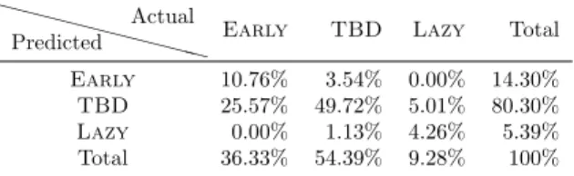
We start by assessing the quality of our partitioning of blocks into Early, Lazy, and TBD in Table 2 using matrix Geo1438 which includes 56727 com-pressible (large enough) blocks. The training was performed using matrix Serena and the low-rank tolerance used for both matrices is 10−8. This ta-ble leads to mixed conclusions. One the one hand, the number of actual Early blocks predicted as Lazy, and the number of actual Lazy blocks predicted as Early is negligible (3 in total). On the other hand, only 45.95% of the actual Lazy blocks are predicted as such, and 29.61% of the actual Early blocks are predicted as such. Moreover, 8.58% of the actual TBD blocks are predicted to be either Early or Lazy. Overall, the results presented by Table 2 are therefore far from being random results, but they are also not perfect and the approxi-mation algorithm will have to process significantly more blocks than required if we had a perfect oracle.
XX XX XX XXX X Predicted Actual
Early TBD Lazy Total
Early 10.76% 3.54% 0.00% 14.30%
TBD 25.57% 49.72% 5.01% 80.30%
Lazy 0.00% 1.13% 4.26% 5.39%
Total 36.33% 54.39% 9.28% 100%
Table 2: Statistics on the classification of blocks according to their actual and predicted characteristics.
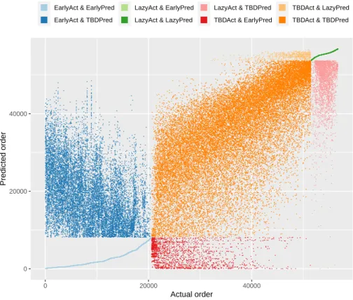
In Figure 3 we compare the ordering of all blocks when using either the actual characteristics of blocks or the predicted ones. For both sets of characteristics, Early blocks are ordered first, then the TBD blocks, and finally the Lazy blocks. The TBD blocks are obviously ordered according to the Ti−ti
Si−si ratio. The
other blocks are (arbitrarily) ordered using the block identifiers. This explains why the set of correctly predicted Early blocks forms a (light blue) line on the graph, and so do the correctly predicted Lazy blocks (dark green line). In this figure blocks are colored according to both their actual (suffix “Act”) and predicted (suffix “Pred”) types.
Once again, the conclusions are mixed. On the one hand, this figure does not look at all like a random figure (where sub-rectangles would be uniformly filled). For instance, the mislabelled actual Early blocks (dark blue dots) appear rather “early” in the overall order and the mislabelled actual Lazy blocks (pink dots) appear mostly very late in the order. Also, one can guess a trend looking like a diagonal for the actual TBD blocks that are correctly predicted (dark orange
dots).
On the other hand, one could argue that the clouds of points show huge variations in the ordering of some blocks. One might wonder, however, whether changing the position of a block in the ordering by 1000 (or 5000) positions in a list of more than 56000 blocks really matters. The actual question is whether such mixed results for the ordering of blocks can still lead to an efficient heuristic in practice. (As we dared to submit this paper, the reader can guess that the answer to that question is positive, at least in our minds.)
As a side note, we remark that, in practice, the quality of the solution produced by Algorithm 1 is not distinguishable from the quality of the optimal solution. 0 20000 40000 0 20000 40000 Actual order Predicted order
EarlyAct & EarlyPred EarlyAct & TBDPred
LazyAct & EarlyPred LazyAct & LazyPred
LazyAct & TBDPred TBDAct & EarlyPred
TBDAct & LazyPred TBDAct & TBDPred
Figure 3: Comparison of the actual and predicted orders of blocks, under Algo-rithm 1.
5
Experiments
We now present the results of our memory-aware strategy. In Section 5.1, we present the machine as well as the matrices used for the experiments. In
Section 5.2, we detail the implementation of the memory-aware strategy. In Section 5.3, we demonstrate the potential of the method. In Section 5.4, we comment on the implementation of this approach into the PaStiX solver before detailing results on factorization time in Section 5.5.
5.1
Experimental context
Experiments were performed on the crunch cluster from our LIP laboratory, where a node is equipped with four Intel Xeon E5-4620 8-cores running at 2.20 GHz and 378 GB of memory. On this platform, the Intel MKL 2018 library is used for sequential BLAS and LAPACK kernels. The PaStiX version used for our experiments is based on the public git repository3 version at the
tag 6.1.0. Large column blocks are split in order to obtain column blocks of width between 128 and 256. Blocks with a width larger or equal to 128 and a height larger or equal to 20 are set to compressible. In all those experiments, a 10−8 tolerance has been used.
In order to validate the results for representative real-life problems, we have used five 3D matrices extracted from The SuiteSparse Matrix Collection [21]:
• Atmosmodl: atmospheric model (1 489 752 non-zeroes)
• Flan1565: 3D mechanical problem discretizing a steel flange (1 564 794 non-zeroes)
• Geo1438: geomechanical model of earth (1 437 960 non-zeroes) • Hook1498: model of a steel hook (1 498 023 non-zeroes) • Serena: gas reservoir simulation (1 391 349 non-zeroes)
Note that these matrices come from different application fields and have thus different mathematical properties. Therefore, training the model on a matrix and using it for another matrix will test not only the efficiency of the model, but also the robustness of our overall approach. Our objective here is to predict memory consumption and computational cost using the models presented in Section 4.2 and Section 4.3, and to use these values to select which blocks to execute in lazy mode in order to use as much memory as possible without overcoming a given memory limit.
5.2
Implementation of the memory-aware strategy
In this section, we present how we solve the MakespanWithBoundedMemory problem presented in Section 3 in practice. The choice of the mode for blocks (early or lazy) is done in a dynamic way before their allocation in the memory. We describe in detail the approach below.
3
1. For both training and test matrices, we run the real factorization using Just-In-Time and Minimal Memory strategies for all blocks. Then we extract information for each elementary update, using results of the Mini-mal Memory (respectively Just-In-Time) for the early (resp. lazy) mode. We perform three runs and take the median value to remove data noise before training the model. Then, we compute the rank model and both time models;
2. We select blocks that should always be treated in lazy mode (si≥ Si) as
well as blocks that should always be treated in early mode (ti≥ Ti);
3. We sort the remaining blocks with the greedy algorithm presented in Al-gorithm 1 by decreasing value of Ti−ti
Si−si;
4. We consider all remaining blocks in lazy mode (uncompressed), which would all require Si if allocated in memory. Then, some blocks are
com-pressed (and thus moved to the early mode) following the previous order until the memory limit is achieved. The memory consumption of the cur-rent solution is computed as the sum of Si for blocks still in the lazy mode
plus the sum of the si for blocks moved to early mode. Note that we use
the real size si and not the predicted one: it is known as soon as a block
is compressed (and it is more accurate than the predicted one). When the memory of the current solution falls below the memory limit, blocks still in lazy mode may safely be loaded.
5.3
Potential gain estimation through simulation
In order to validate the models presented in Section 4, we have implemented the previous approach using different ordering strategies for Step 3. From now on, we denote by Ti, ti, and sithe actual timings and memory consumption and
Ti∗, t∗i, and s∗i the predicted ones. The four orderings are: • Decreasing theoretical ratio Ti−ti
Si−si (this is to get a bound on the best
result we can obtain with our models). • Decreasing predicted ratio Ti∗−t∗
i
Si−s∗i
(original strategy).
• Decreasing number of updates received by a block: we expect blocks re-ceiving many updates to be more efficient in lazy mode, to avoid numerous expensive low-rank updates (denoted by count in the following figures). This strategies does not rely on predicted values, and is thus simpler to implement.
• Random order, for baseline comparison.
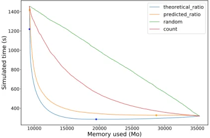
On Figure 4, we present the results of the four heuristics for the Geo1438 matrix. The training of the models was realized with the Serena matrix. Both matrices were studied with a 10−8 tolerance. For each possible memory limit,
10000 15000 20000 25000 30000 35000
Memory used (Mo)
400 600 800 1000 1200 1400
Simulated time (s)
theoretical_ratio
predicted_ratio
random
count
Figure 4: Simulated time of update tasks depending on the memory constraint for Geo1438 solved with a 10−8 tolerance for four different heuristics. The training matrix for the predictive strategy is Serena using a 10−8 tolerance. The top-left point represents the Minimal Memory strategy while the bottom-right point represents the Just-In-Time strategy.
we run the previous algorithm to decide which mode to use for each block. Note that here, the time is simulated and corresponds only to the sum of update times; the cost of common operations (remaining kernels of the considered blocks as well as all operations on small full-rank blocks such as the factorization of diagonal blocks) is omitted for better readability. The update times are extracted from the training data set, as explained above. On top-left part of the figure, we have the largest execution time and the lowest memory consumption: it corresponds to performing all blocks under the early mode, which is exactly the Minimal Memory strategy. On bottom-right, we have the opposite case, using lazy mode for all blocks, which is exactly the Just-In-Time strategy, with the largest memory consumption but the lowest execution time. Four points appear on the figure, two for the “theoretical ratio” and two for “predicted ratio”. The points on the left represent the lowest execution time achievable under the condition of using as low memory as possible: all blocks are executed in early mode except those which do not bring memory savings (si ≥ Si or
s∗i ≥ S∗
i) that are processed in lazy mode. On the contrary, the two right points
represent the lowest memory consumption under the condition of being as fast as possible: all blocks are executed in lazy mode except those which are faster in early mode (ti≥ Ti or t∗i ≥ Ti∗).
Between those two points, one can observe all possible combinations for the memory-aware strategy. The first observation is that, while being not as good as the best ratio available, the prediction leads to much better results than a naive sorting such as the number of updates. In addition, one can see that interesting trade-offs between time and memory can be achieved: for instance by increasing memory consumption by only 20%, execution time can be divided by 3.
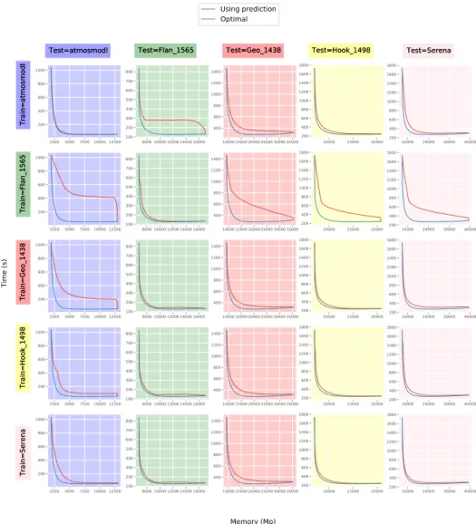
On Figure 5, one can observe the behavior of the best ratio and the pre-dictive one for the 25 combinations. Among the five matrices we used for our experiments, we vary both the training and the testing sets, always using a 10−8 tolerance. This demonstrates that the results using the predictive models are often or always close to the optimal solution. This prove that our approach is very robust to the choice of the training matrix. They are similar to Figure 4 and show the robustness of our approach.
5.4
Integration of the memory-aware strategy into the
PaStiX solver
Based on these attractive preliminary results, we now present how this memory-aware strategy has been introduced into the PaStiX solver and the gains ob-tained on actual factorization time and memory usage.
The first step consists of selecting blocks which will be performed in the early mode, such that the memory consumption of the factors before the fac-torization starts is below the given memory limit. Then, we have two opposite behaviors during the factorization. On one hand, once blocks which are man-aged in lazy mode have received all their contributions (cf. Figure 2(e)), they can be compressed, reducing the memory footprint of the solver. On the other
2500 5000 7500 10000 12500 200 400 600 800 1000 8000 10000 12000 14000 16000 100 200 300 400 500 600 700 800 100001500020000250003000035000 400 600 800 1000 1200 1400 10000 15000 20000 200 400 600 800 1000 1200 1400 1600 1800 10000 20000 30000 40000 200 400 600 800 1000 1200 1400 1600 1800 2500 5000 7500 10000 12500 200 400 600 800 1000 8000 10000 12000 14000 16000 100 200 300 400 500 600 700 800 100001500020000250003000035000 400 600 800 1000 1200 1400 10000 15000 20000 200 400 600 800 1000 1200 1400 1600 1800 10000 20000 30000 40000 200 400 600 800 1000 1200 1400 1600 1800 2500 5000 7500 10000 12500 200 400 600 800 1000 8000 10000 12000 14000 16000 100 200 300 400 500 600 700 800 100001500020000250003000035000 400 600 800 1000 1200 1400 10000 15000 20000 200 400 600 800 1000 1200 1400 1600 1800 10000 20000 30000 40000 200 400 600 800 1000 1200 1400 1600 1800 2500 5000 7500 10000 12500 200 400 600 800 1000 8000 10000 12000 14000 16000 100 200 300 400 500 600 700 800 100001500020000250003000035000 400 600 800 1000 1200 1400 10000 15000 20000 200 400 600 800 1000 1200 1400 1600 1800 10000 20000 30000 40000 200 400 600 800 1000 1200 1400 1600 1800 2500 5000 7500 10000 12500 200 400 600 800 1000 8000 10000 12000 14000 16000 100 200 300 400 500 600 700 800 100001500020000250003000035000 400 600 800 1000 1200 1400 10000 15000 20000 200 400 600 800 1000 1200 1400 1600 1800 10000 20000 30000 40000 200 400 600 800 1000 1200 1400 1600 1800 Test=atmosmodl Train=atmosmodl Test=atmosmodl Train=atmosmodl Train=Flan_1565Train=Flan_1565 Train=Geo_1438Train=Geo_1438 Train=Hook_1498Train=Hook_1498 Train=SerenaTrain=Serena Test=Flan_1565
Test=Flan_1565 Test=Geo_1438Test=Geo_1438 Test=Hook_1498Test=Hook_1498 Test=SerenaTest=Serena
Memory (Mo)
Time (s)
Using prediction Optimal
Figure 5: Execution time of update tasks depending on the memory constraint for five matrices using a 10−8tolerance. For each line, the same training matrix is used and for each column the same test matrix is used. Two curves are plotted, the best results achievable knowing all information and the results obtained by our predictive models.
hand, low-rank blocks managed under early mode can see their rank increase due to updates (cf. Figure 2(d)), increasing the memory footprint. Thus, to ensure that we always stay under the memory limit, each time a low-rank block size increases, some extra blocks may be moved dynamically to early mode and compressed if the extra memory allocated would exceed the given limit.
This implementation is a proof-of-concept and has some limitations. Firstly, it is only sequential for now, as compressing on-the-fly data blocks may induce deadlocks when using PaStiX in parallel. Secondly, building and using the models as well as sorting blocks is performed using an external tool. In future work, it will be fully integrated into the PaStiX solver, and a parallel memory management will be proposed.
5.5
Real gain for the PaStiX solver
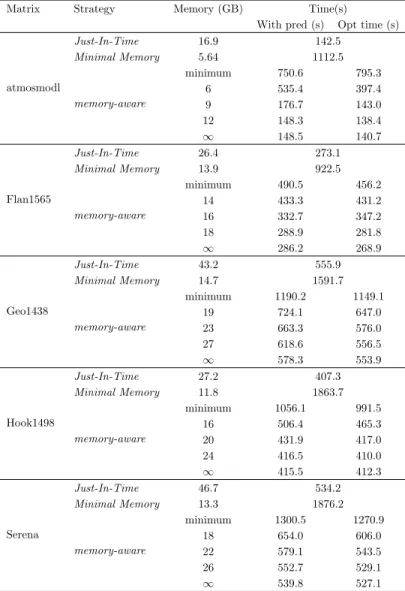
With the implementation presented before, we can now compare the behavior of both Just-In-Time and Minimal Memory strategies with the memory-aware method introduced in this paper. This requires to add an extra entry parameter to the PaStiX solver, the maximum memory authorized.
In Table 3 we present, for five matrices solved at tolerance 10−8, the memory consumption and factorization time for the Just-In-Time and Minimal Memory strategies. The models were trained using the Serena matrix with a 10−8 tol-erance. We evaluate the memory-aware strategy with different memory limits, as well as two extreme cases: all blocks executed in early mode except those which do not bring memory savings (denoted minimum) and all blocks exe-cuted in lazy mode except those which do not reduce execution time (denoted ∞). We present both the optimal time (using actual values from the execution) and the time achieved using the predictive models. The results demonstrate that an interesting trade-off between time and memory can always be achieved. For instance, for the Geo1438 matrix, increasing memory consumption by 30% divides by 2.2 the execution time of Minimal Memory strategy. Similarly, 60% of the memory consumption of the Just-In-Time strategy could be saved by increasing by only 10% the execution time. Using the predictive values we are always within 10% of the optimal performance.
6
Conclusion
In sparse direct solvers, using low-rank compression has emerged as a solution to process larger matrices. Existing solvers use either only low-rank updates (the matrix is compressed beforehand) or only full-rank updates (the matrix is compressed during the factorization). We have presented a memory-aware approach, performing both types of updates, whose objective is to enable ap-plications to run as fast as possible while keeping their memory usage under a given memory limit (e.g., the size of the RAM).
We have formalized the optimization problem of choosing which blocks to compress in the early or lazy mode, and shown its equivalence to the knapsack
problem, which proves our problem NP-complete. We have successfully adapted a 2-approximation algorithm for our problem.
To take advantage of this optimization algorithm, we need information on matrix blocks (memory consumption once compressed, processing time in both modes) which is usually unknown before the computation. To leverage this prob-lem, we have introduced models to predict these values. We have demonstrated that using these models we can achieve a performance close to the results achiev-able with a perfect omniscient oracle, even in the less favorachiev-able case where the models are trained with a matrix from one application field and used with ma-trices from another field. Our approach sorts all blocks and selects at runtime, depending on the actual memory usage, which ones to manage with low-rank updates (early mode) and which ones to manage with full-rank updates (lazy mode). This ensures that the memory bound is respected.
Our memory-aware strategy has been integrated into the PaStiX solver. The obtained execution times are far lower than the existing memory-conservative strategy (for instance, twice faster), even for memory limits that are only slightly larger than the memory usage of this strategy (for instance, 30% increase in memory). Conversely, it is only marginally slower than the performance-oriented strategy (for instance, 10% increase in execution time) while using drastically less memory (for instance, half the memory). The memory-aware strategy thus achieves a kind of “best of both world” performance, allowing a wide range of memory-time trade-offs.
The implementation is for now sequential and the memory management has to be adapted for the parallel case, which is left for future work. The main problem here is to avoid deadlocks, as the next candidate for being compressed may be used by another thread, for instance to apply an update. The work conducted in [22] could be a starting point.
Another future work consists of using geometric information of the matrix, which is known to influence ranks, to try to enhance the predictive models of processing times and memory consumption.
Up to our knowledge, this work is the first tentative to produce models for low-rank compression in the sparse case. It could be used to exhibit better time estimation to enhance scheduling for sparse direct solvers using low-rank compression.
Acknowledgments
This work is part of the SOLHARIS project, supported by the Agence Nationale de la Recherche, under grant ANR-19-CE46-0009.
References
[1] P. R. Amestoy, C. Ashcraft, O. Boiteau, A. Buttari, J.-Y. L’Excellent, and C. Weisbecker, “Improving Multifrontal Methods by Means of Block
Low-Rank Representations,” SIAM Journal on Scientific Computing, vol. 37, no. 3, pp. A1451–A1474, 2015.
[2] T. Mary, “Block Low-Rank multifrontal solvers: complexity, performance, and scalability,” Ph.D. dissertation, Toulouse University, Toulouse, France, Nov. 2017.
[3] G. Pichon, “On the use of low-rank arithmetic to reduce the complexity of parallel sparse linear solvers based on direct factorization techniques,” Ph.D. dissertation, Universit´e de Bordeaux, Talence, France, Nov. 2018. [4] W. Hackbusch, “A Sparse Matrix Arithmetic Based on H-Matrices. Part I:
Introduction to H-Matrices,” Computing, vol. 62, no. 2, pp. 89–108, 1999. [5] W. Hackbusch and S. B¨orm, “Data-sparse Approximation by Adaptive H2
-Matrices,” Computing, vol. 69, no. 1, pp. 1–35, 2002.
[6] P. Ghysels, X. S. Li, C. Gorman, and F.-H. Rouet, “A robust parallel preconditioner for indefinite systems using hierarchical matrices and ran-domized sampling,” in 2017 IEEE IPDPS, 2017, pp. 897–906.
[7] A. Aminfar and E. Darve, “A fast, memory efficient and robust sparse pre-conditioner based on a multifrontal approach with applications to finite-element matrices,” International Journal for Numerical Methods in Engi-neering, vol. 107, no. 6, pp. 520–540, 2016.
[8] T. A. Davis, R. Sivasankaran, and W. M. Sid-Lakhdar, “A survey of direct methods for sparse linear systems,” Acta Numerica, vol. 25, pp. 383–566, 2016.
[9] A. George, “Nested dissection of a regular finite element mesh,” SIAM Journal on Numerical Analysis, vol. 10, no. 2, pp. 345–363, 1973.
[10] G. Karypis and V. Kumar, “METIS: A software package for partitioning unstructured graphs, partitioning meshes, and computing fill-reducing or-derings of sparse matrices,” 1995.
[11] F. Pellegrini, “Scotch and libScotch 5.1 User’s Guide,” Aug. 2008, user’s manual, 127 pages.
[12] J. J. Dongarra, J. Du Croz, S. Hammarling, and I. S. Duff, “A set of level 3 basic linear algebra subprograms,” ACM Trans. Math. Softw., vol. 16, no. 1, pp. 1–17, 1990.
[13] P. H´enon, P. Ramet, and J. Roman, “PaStiX: A High-Performance Parallel Direct Solver for Sparse Symmetric Definite Systems,” Parallel Computing, vol. 28, no. 2, pp. 301–321, Jan. 2002.
[14] J. N. Chadwick and D. S. Bindel, “An Efficient Solver for Sparse Linear Systems Based on Rank-Structured Cholesky Factorization,” CoRR, vol. abs/1507.05593, 2015.
[15] J. E. Savage, Models of computation - exploring the power of computing. Addison-Wesley, 1998.
[16] L. Marchal, “Memory and data aware scheduling,” Habilitation Thesis, ´
Ecole Normale Sup´erieure de Lyon, 2018.
[17] H. Kellerer, U. Pferschy, and D. Pisinger, “Multidimensional knapsack problems,” in Knapsack problems. Springer, 2004, pp. 235–283.
[18] E. Tardos, “Introduction to approximation and online algorithms,” avail-able online at http://www.cs.cornell.edu/courses/cs4820/2018fa/lectures/ approx-onlinet.pdf, course note of CS 4820 Spring 2016 ”Introduction to Algorithms” at Cornell University.
[19] S. Ubaru and Y. Saad, “Fast methods for estimating the numerical rank of large matrices,” in ICML, 2016, pp. 468–477.
[20] L. Stanisic, E. Agullo, A. Buttari, A. Guermouche, A. Legrand, F. Lopez, and B. Videau, “Fast and accurate simulation of multithreaded sparse lin-ear algebra solvers,” 2015 IEEE ICPADS, 2015.
[21] T. A. Davis and Y. Hu, “The University of Florida sparse matrix collec-tion,” ACM Trans. Math. Softw., vol. 38, no. 1, Dec. 2011.
[22] M. Sergent, D. Goudin, S. Thibault, and O. Aumage, “Controlling the Memory Subscription of Distributed Applications with a Task-Based Run-time System,” in HIPS, Chicago, IL, May 2016.
Table 3: Factorization time and memory consumption for five matrices solved at tolerance 10−8. For each matrix, the results of both Just-In-Time (JIT) and Minimal Memory (MM) are presented as well as the results for different memory-aware strategies where the memory limit varies. For the memory-aware strategy, the predictive model is obtained using Serena as training test. Two information are provided, the best result achievable knowing all information and the result obtained using our predictive model.
Matrix Strategy Memory (GB) Time(s)
With pred (s) Opt time (s)
atmosmodl Just-In-Time 16.9 142.5 Minimal Memory 5.64 1112.5 memory-aware minimum 750.6 795.3 6 535.4 397.4 9 176.7 143.0 12 148.3 138.4 ∞ 148.5 140.7 Flan1565 Just-In-Time 26.4 273.1 Minimal Memory 13.9 922.5 memory-aware minimum 490.5 456.2 14 433.3 431.2 16 332.7 347.2 18 288.9 281.8 ∞ 286.2 268.9 Geo1438 Just-In-Time 43.2 555.9 Minimal Memory 14.7 1591.7 memory-aware minimum 1190.2 1149.1 19 724.1 647.0 23 663.3 576.0 27 618.6 556.5 ∞ 578.3 553.9 Hook1498 Just-In-Time 27.2 407.3 Minimal Memory 11.8 1863.7 memory-aware minimum 1056.1 991.5 16 506.4 465.3 20 431.9 417.0 24 416.5 410.0 ∞ 415.5 412.3 Serena Just-In-Time 46.7 534.2 Minimal Memory 13.3 1876.2 memory-aware minimum 1300.5 1270.9 18 654.0 606.0 22 579.1 543.5 26 552.7 529.1 ∞ 539.8 527.1
Inovallée
655 avenue de l’Europe Montbonnot
BP 105 - 78153 Le Chesnay Cedex inria.fr