Thermal field pr
Thermal field prediction in DED manuf
ediction in DED manufacturing pr
acturing process using Artificial Neur
ocess using Artificial Neural
al
Netw
Networ
orkk
Seifallah Fetni, Quy Duc Thinh Pham, Van Xuan Tran, Laurent Duchêne, Hoang Son Tran and Anne Marie Habraken Seifallah Fetni.University of Liège, UEE Research Unit, MSM division, allée de la Découverte, 9 B52/3, B 4000 Liège, Belgium Quy Duc Thinh Pham.Thu Dau Mot University, Vietnam
University of Liège, UEE Research Unit, MSM division, allée de la Découverte, 9 B52/3, B 4000 Liège, Belgium Van Xuan Tran.Thu Dau Mot University, Vietnam
Corresponding author:[email protected]
Laurent Duchêne.University of Liège, UEE Research Unit, MSM division, allée de la Découverte, 9 B52/3, B 4000 Liège, Belgium Hoang Son Tran.University of Liège, UEE Research Unit, MSM division, allée de la Découverte, 9 B52/3, B 4000 Liège, Belgium Anne Marie Habraken.University of Liège, UEE Research Unit, MSM division, allée de la Découverte, 9 B52/3, B 4000 Liège, Belgium
Fund of Scientific Research F.R.S-FNRS A
Abstrbstractact.. In the last decade, machine learning is increasingly attracting researchers in several scientific areas and, in particular, in the additive manufacturing field. Meanwhile, this technique remains as a black box technique for many researchers. Indeed, it allows obtaining novel insights to overcome the limitation of classical methods, such as the finite element method, and to take into account multi-physical complex phenomena occurring during the manufacturing process. This work presents a comprehensive study for implementing a machine learning technique (artificial neural network) to predict the thermal field evolution during the direct energy deposition of 316L stainless steel and tungsten carbides. The framework consists of a finite element thermal model and a neural network. The influence of the number of hidden layers and the number of nodes in each layer was also investigated. The results showed that an architecture based on 3 or 4 hidden layers and the rectified linear unit as the activation function lead to obtaining a high fidelity prediction with an accuracy exceeding 99%. The impact of the chosen architecture on the model accuracy and CPU usage was also highlighted. The proposed framework can be used to predict the thermal field when simulating multi-layer deposition.
K
Keeywyworordsds. Machine Learning, Artificial Neural Network, Direct Energy Deposition, Thermal Model
1 Intr
1 Introduction
oduction
Additive Manufacturing (AM) processes are today widely spread and prove their ability to form complex shapes and are applied on a wide variety of alloys [1,2]. Meanwhile, industrial applications face various kinds of defects during and after fabrication: porosity, formation of cracks, keyhole defects [3], difficulties to produce net shapes etc. This is due to the complex phenomena occurring during the manufacturing process.
Experimentations and trials constitute a way to adjust process parameters (laser power, scanning speed, spot size, building direction, hatch spacing, feed rate, distance nozzle-substrate etc.) but are time and cost consuming. Therefore, numerical techniques, in particular the Finite Element Method (FEM), have been used as promising tools to predict various outputs such as microstructure, mechanical properties, melt pool shape, and dimensions.
Within literature, several approaches to model AM processes have been developed [4-8]. These numerical models help to better optimize process parameters and offer the possibility for industrials to reasonably predict distortions, shapes, residual stresses, thermal histories etc. However, numerical modeling applied on AM still faces various challenges. Indeed, multi-physical simulations are time and CPU consuming and require simplifying assumptions, which result
additional high cost must be paid; taking in account real thermo-physical properties of the cladded materials, multi-technique validations : thermocouple records, high speed cameras, microstructural analysis, nano-indentations…Thus, simulation should be validated by at least two techniques [8,9]. Boundary conditions are still a serious challenge in AM modeling due to the difficulty of experimental measurements. These FEM drawbacks trigger scientists to look for alternative approaches.
Machine Learning (ML) is a promising technique which has been enhanced by the increasing computing capacity, mostly in the last decade [10]. It trends to prove its ability to be complementary and even substitute for traditional techniques in computational material science. It has been considered as a technology development accelerator in various fields like chemistry, molecule design [11], finance [12], Web … but is still a new approach in materials science and especially in the field of metals. The limitation of ML in this research area is due to the lack of large dataset of materials, while other domains take advantage of large available datasets: Kaggle, AWS, Socrata, etc. Most recently, Integrated Computational Materials Engineering (ICME) approach has been developed to enhance emergence of new materials and better selection, especially in advanced applications. The aim is to develop a strong network relating actors in material science field. ML framework provides a good opportunity to couple ICME tools and experimentations [10]. Researchers in AM field are giving increasing attention to harness the benefits of Artificial Intelligence (AI) in order to optimize materials design and control process parameters. It should be noted that ML is the set of soft techniques applied to realize AI. AI approaches can be classified into two main groups: supervised and unsupervised learning. Supervised learning is used in case of known responses and englobes regression algorithms on the one hand and classification ones on the other hand, while unsupervised learning is used in case of unknown response (prediction, recognition, etc.). Regression techniques in AM field have the aim to predict continuous responses (thermal histories [13], melt pool depth [14], deformations [15], etc.). For that, linear or nonlinear regressions, Gaussian Process (GP), Support Vector Machine (SVM), Logistic and Artificial Neural Networks (ANN) are good candidates. Classification techniques are attracting attention of material’s researchers to predict various defects occurring during manufacturing such as abnormal grain growth. For that, K-nearest neighbors, Logistic regression and SVM are strongly recommended according to [16].
The selection of the appropriate algorithm strongly depends on a variety of criteria such as the size of the training data, memory usage, target accuracy, interpretability of results and number of features. Statistical methods and pure-data-driven models are developed in AM field to quantify the influence of process parameters on mechanical properties, surface characteristics, build shape, etc.
Within literature, some interesting ML models applied on AM of metals can be highlighted. Tapia et al. [14] developed a framework based on a GP surrogate model to predict melt pool depth in single track Laser Powder-Bed Fusion (L-PBF) deposition of 316L Stainless Steel (SS). The model was used to identify appropriate process parameters to get the desirable heat conduction and reduce keyhole mode effects. Waqas et al. [17] proposed a model of the deposition of AlSi10Mg alloy by Selective Laser Melting (SLM) in order to predict plastic anisotropy, local strain distribution and failure in tensile tests.
As the application of ML in AM field is still not widely applied in particular in metal alloys and is often considered as a black box for several researchers of this field, this work proposes an exploratory and comprehensive study that highlights the methodology of implementation of an AI framework composed of a physically based model (FEM) and an ANN algorithm. An initial architecture was chosen through trial and error as a first step. Then, different configurations were studied with varying numbers of hidden layers, numbers of nodes per hidden layers and activation functions.
2 FEM model and ML fr
2 FEM model and ML framew
amewor
orkk
2.1
FEM model
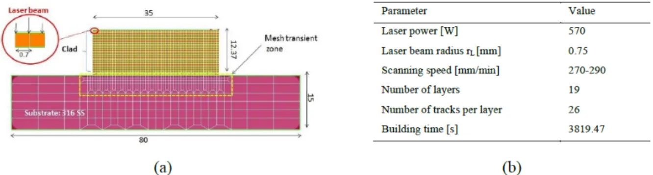
A FEM model for 2D thermal simulation of the Directed Energy Deposition (DED) of the composite coating (316L SS and tungsten carbides) was developed to predict the thermal history during the building stage and to get insights about possible microstructures of the solidified material [18]. The 2D model is shown in Fig. 1. The clad consisted in 19 superimposed layers. The validation of the model was based on two validation criteria: measured melt pool depths and a substrate thermocouple records. In addition to the parameters gathered in Fig. 1b, thermo-physical properties and boundaries conditions (radiation and convection) were considered [18].
Fig. 1. (a) The 2D mesh designed f
Fig. 1. (a) The 2D mesh designed for the thermal field of DED deposition of 316L SS+ Tor the thermal field of DED deposition of 316L SS+ Tungstungsten caren carbides and (b) thebides and (b) the set of pr
set of process and simulation input data [18].ocess and simulation input data [18].
2.2
2.2
ANN model
ANN model
From ML regression techniques, which predict continuous responses such as temperature field history, ANN was here chosen. This choice is recommended for highly non-linear problems and consists in fully connected perceptrons to mimic the human brain. The thermal history predicted by the FEM model was used as the input data of ANN. Input dataset, organized as a matrixX, is indeed composed of following input features: 𝑋=(𝑥 𝑦 𝑡 𝑥𝐿𝑦𝐿𝑑𝑥𝑑𝑦)𝑇;x, y are the coordinates,t is the FE time step, xLandyLdefine the laser position at each Finite Element (FE) time step,dxanddy are the distance between laser head and each point P(x,y) at each time step. It was reported that the distance between laser head and substrate points has direct impact on their thermal history and melt pool shape [19]. Overall, the input matrixXX has 7 as columns number (7 input features) and the output layer contains nodal temperature for each point at each FE time step.
It should be noted that the case where the matrix only consists inx, y and t as input was also investigated in order to highlight the impact of adding more features on the model accuracy. In a related work, input laser power (input energy) was varied in the FEM model to get a bigger dataset and was considered in the input matrix. Moreover, the layer number was taken into account [20].
The actual work took into account only one FEM simulation due to its exploratory purpose. The ANN architecture was first chosen using trials and error which led to 4 hidden layers; each one contains 100 nodes, as shown in Fig. 2 and Table 1. The neural network computing was executed in two main steps. The first step is the feedforward. The impact of the input features on output results (nodal temperatures) is to be initiated through random weights affected to the connections between nodes. The computed value at each node is a weighted sum to which the activation function
here a is the output value of a given perceptron,f is the activation function (often non-linear), withe weight of an input connexion i whose value is xiand b the bias. The activation functions are various such as the Rectified Linear Unit (Relu), Logistic (sigmoid), the hyperbolic tangent (tanh), and the softmax (also called softargmax) [17,11].
Fig.1 Ar
Fig.1 Architchitecturecture of the pere of the perceptrceptron (a) and the ANN model (b).on (a) and the ANN model (b). TTable 1. Description of the implementable 1. Description of the implemented model.ed model.
It should be noted that this architecture corresponds to deep learning, as the number of hidden layers exceeds one. The data preprocessing was ensured by feature transformation integrated into the single matrix (X) then normalized. Indeed, normalization is a key step in data preparation to allow the ML algorithm a better modeling of the data. In particular, the data was normalized to the range of 0 and 1. A Python script code was used to implement the framework using the free scientific libraries: Numpy (high dimensional arrays and matrix), Scipy (scientific computing), Matplotlib (graphics), Pandas (data analysis), Tensorflow (differential programming and data flow), Keras (interface for ANN), Sklearn (data regression) and Shap (feature importance). Using the Keras sequential model, the input data were divided into a training data set and a validation one through the choice of 0.6 as ratio (ts). The ANN model was trained using only 60% of input data, while the remaining 40% were used to validate the model. Data normalization was processes using the sklearn object “MinMaxScaler”.
3 R
3 Results and discussion
esults and discussion
After the training and validation phases, predicted ANN solutions were compared to those obtained by FEM simulations. Thermal histories for selected important material points (gathered in Fig. 3a) were carried out. These points were selected from different heights of the clad, at the beginning of the deposition and from the substrate. For comparison purposes, various metrics evaluate the ML model performances called loss fucntions. The mean squared error (MSE) is given by the formula:
The mean absolute error (MAE) is expressed by:
These errors were used to evaluate the accuracy of regression problems. Here yi, ŷ𝑖 and n are respectively the reference value (FEM result), the predicted one (ANN) and the number of samples or rows in the validation dataset (ts*nb_node * nb_time_steps). MSE has the advantage of providing a quadratic loss function and letting data scientist punish big errors, but that may enhance difficulty of interpretability by varying from 0 to infinity. MAE simply gives the absolute difference between actual (from FEM model) and predicted values (by ANN), but is an absolute value like MSE. The Mean Absolute Percentage Error (MAPE) is suitable for regression problems and has the advantage to be more interpretable as it is a relative error. It is given by the formula:
Likewise, the R2score is interpretable as it varies between 0 and 1. It links the variance from the model to the total variance through the relationship:
where 𝑦̅𝑖is the mean of actual values. The more data are correlated, the more the tendency of R2is to be close to 1. It was here chosen to begin by highlighting results of the ANN model when onlyx, y and t are considered. As inferred from Fig.3 b, there is a discrepancy between FEM results and ANN prediction. This is mainly expressed by a MAPE higher than 7%. This finding is also reported for other material points. Moreover, the oscillation profile is not captured by the ANN model. The model accuracy calculation is based mainly on these different loss functions (𝑅2, 𝑀𝑆𝐸, 𝑀𝐴𝐸 𝑎𝑛𝑑 𝑀𝐴𝑃𝐸), as well as the model error hereafter defined.
Fig.3 a: SelectFig.3 a: Selected mated material points (ferial points (for comparison purposes). b: Comparison betwor comparison purposes). b: Comparison between actual (FEM) Preen actual (FEM) Predictedicted (ANN) fed (ANN) foror P2 (middle of the clad)P2 (middle of the clad)
When considering all features (7 inputs), there is a good agreement between FEM and ANN predicted curves, as shown in Fig. 4. The model loss is a number indicating how well the model is doing. It was computed for each example in training and validation sets. The lower is the loss, the better is the model. Fig. 4a shows the good trend of the loss functions. At the beginning of the deposition, temperature peaks are not well captured by ML (P0). By increasing time, MSE, MAE, MAPE tend to decrease, while the 𝑅2score tends to increase. MAPE, which gives interpretable values, decreases from 2.93% for the thermal history of P0 to reach 1.29% for those of P3. The model loss presents a good tendency and final value.
Fig.4 Model loss (a) and comparison betw
Fig.4 Model loss (a) and comparison between preen predictedicted thermal histed thermal history of selectory of selected points using FEM and ANNed points using FEM and ANN appr
approaches [(b) toaches [(b) to (e) ] wo (e) ] when taking in account all fhen taking in account all featureatures.es.
The test accuracy is higher than 99%, which suggests a high fidelity model. Output data were postprocessed for a better visualization. As shown in Fig.5, the ANN model predicted a thermal field distribution similar to that predicted from the FEM model. The big data set (training and validation) explains the high fidelity prediction. Indeed, it consists of 4079768 samples (1628 nodes * 2506 time steps). Moreover, the most influential parameters, such as laser power, idle time, distance from substrate to nozzle as well as the geometry were not varied. That allows ANN a good modeling
of data without too much training time.
Fig.5. Thermal fields comput
Fig.5. Thermal fields computed bed by FEM (a) and pry FEM (a) and predictedicted bed by ANN (b). The melt pool corry ANN (b). The melt pool corresponds tesponds to the black aro the black areaea w
wherhere te temperemperaturature is aboe is abovve 1720 K (liquidus).e 1720 K (liquidus).
This study was exploratory. It is hereafter proposed to highlight the impact of the architecture of the sequential ANN model on the prediction accuracy. It is reminded that this architecture is based on the number of hidden layers, the number of nodes for each one and the activation function. Tanh, sigmoid and softmax activation functions were implemented in the model as replacements of Relu. For each case, a mean percentage error is defined as the mean of all MAPE values and is proposed as the model error. Indeed, each MAPE corresponds to a node number and time steps. This mean percentage error allows interpreting accuracies and is proposed hereafter as the model error. Results, given in Fig.6a, confirm the initial choice of Relu which was based on the fact that Relu functions are commonly used in regression problems with neural networks [21]. The huge error given by the softmax function was excepted because it is often applied in only the last hidden layer as a classifier, used e.g., in image analysis problems with deep neural networks [18]. Tanh also gives acceptable results for this highly non-linear problem because the data has been normalized to the range of 0 and 1.
Fig.6. Impact of the chosen acti
Fig.6. Impact of the chosen activvation function (a) and of the number of hidden laation function (a) and of the number of hidden layyers (HL) (b) on the accurers (HL) (b) on the accuracy of theacy of the model (e
model (exprxpressed bessed by the mean pery the mean percentage errcentage error).or).
For sigmoid, deeper analysis should be applied to interpret the obtained huge error. Indeed, Waqas et al. [17] (see Introduction) had obtained similar losses evolution by applying sigmoid and tanh, when they investigated the effect of the choice of the activation function. In their case, a neural network with 8 hidden layers was selected while 2, 3 and 4 hidden layers (using Relu) were here investigated as shown in Fig. 6b. The performed trials demonstrate that increasing the number of hidden layers leads to progressively reduce the mean percentage error to reach an acceptable value of 2.28%. For comparison purposes, the architecture (8 HL + ”sigmoid” + 100 nodes/HL) was also tried. It
Another interesting analysis consists in testing the effect of the number of the HL nodes on the mean percentage error and the training time. For simplifying purposes, all hidden layers of the model are affected by the same number of nodes (100). As inferred from Fig.7, increasing the number of nodes in the hidden layers leads to progressively decrease the model error to reach a steady value near 2%. It is observed that increasing the number of nodes to greater than 300 does not significantly improve the model error while it can consume significantly more CPU training time. Based on these trials, it could be deduced that an architecture of 3 or 4 hidden layers associated with about 100-200 nodes leads to obtain a good accuracy (more than 99% in this study) and in a reasonable computing time. It should be emphasized that these parameters appeared to be goal for this specific data set and problem.
Fig.7. Impact of the number of nodes (n) on the mean per
Fig.7. Impact of the number of nodes (n) on the mean percentage errcentage error (a) and the tror (a) and the training time (b) faining time (b) for the chosenor the chosen ar
architchitecturecture.e.
Future applications of ML/ANN should be highlighted. For a multi-layer model whose simulation requires too much time to be executed, training an ANN model with few AM layers data would make it able to predict solution for upper layers. Moreover, training the model by varying input parameters (geometry, power, scanning speed etc.) and giving the model the output at each time (thermal field, microstructure, mechanical properties…) gives the possibility to get solutions for other input values without running the computationally cost FEM simulations. The current exercise may be extended to study feature importance, which is an important step in ML modelling and data analysis. Indeed, that allows getting key information about the physically-based or numerical model such as degree of importance of inputs parameters and dependencies between them.
4 Conclusions
4 Conclusions
In this work, a ML framework was proposed consisting in a physically-based FEM model and a deep learning algorithm. The choice of such an architecture was carefully justified. That gave high fidelity prediction for FEM results through more than 99% of accuracy and a model error (mean of all MAPE errors) of about 2% for an ANN model containing 4 HL and 100 nodes/HL. The effect of varying the number of HL and the number of nodes was investigated. The obtained high fidelity is not only explained by the choice of the architecture but also the quantity of input data. Indeed, the deposition of 19 superimposed layers was modeled by FEM, which provided a dataset containing more than 4 million samples.
ANN regression algorithms are well adapted to AM problems because output data are generally continuous such as temperature and strain evolutions. Even if ANN algorithms can substitute FEM through a framework composed of physical analysis and ML model, FEM has the particularity to give big data set alloying ANN to better model input parameters. Thus, combining FEM and ANN in one framework is a suitable choice to get good accuracy. When in-situ control is possible in AM field, real-time computing and adjustment of processing parameters can be possible using ML. Thus, it would be interesting to focus on recurrent neural network algorithms to get better insights of the application
of AI on ML.
A
Ackno
cknow
wledgements
ledgements
As Research Director of the FRS-FNRS, AM Habraken acknowledges the support of this institution.
This work was funded by Vingroup and supported by Vingroup Innovation Foundation (VINIF) under project code VINIF.2020.DA15
Computational resources have been provided by the Consortium des Équipements de Calcul Intensif (CÉCI), funded by the Fonds de la Recherche Scientifique de Belgique (F.R.S.-FNRS) under Grant No. 2.5020.11 and by the Walloon Region
Bibliogr
Bibliograph
aphyy
[1] H-S. Tran , J. T. Tchoufang , H. Paydas , A. Mertens, R. Jardin , L. Duchêne , R. Carrus , J. Lecomte-Bechers , A. M. Habraken, “3D thermal finite element analysis of laser cladding processed Ti-6Al-4V part with microstructural correlations,” Mater. Des., vol. 128, pp. 130–142, 2017
[2] A. Mertens, S. Reginster, H. Paydas, Q. Contrepois, T. Dormal, O. Lemaire, J. Lecomte-Beckers, “Mechanical properties of alloy Ti–6Al–4V and of stainless steel 316L processed by selective laser melting: influence of out-of-equilibrium microstructures,” Powder Metall., vol. 57, no. 3, pp. 184–189, 2014
[3] Chinnapat Panwisawas, Bama Perumal, R. Mark Ward, Nathanael Turner, Richard P. Turner, Jeffery W. Brooks, Hector C. Basoalto, “Keyhole formation and thermal fluid flow-induced porosity during laser fusion welding in titanium alloys: Experimental and modelling,” Acta Mater., vol. 126, pp. 251–263, 2017
[4] E. Toyserkani, A. Khajepour and S. Corbin, “3-D finite element modeling of laser cladding by powder injection: effects of laser pulse shaping on the process,” Opt. Lasers Eng., vol. 41, no. 6, pp. 849–867, 2004,
[5] M. Alimardani, E. Toyserkani, and J. P. Huissoon, “A 3D dynamic numerical approach for temperature and thermal stress distributions in multilayer laser solid freeform fabrication process,” Opt. Lasers Eng., vol. 45, no. 12, pp. 1115– 1130, 2007
[6] A. Hussein, L. Hao, C. Yan, and R. Everson, “Finite element simulation of the temperature and stress fields in single layers built without-support in selective laser melting,” Mater. Des., vol. 52, pp. 638–647, 2013
[7] P. Cadiou, S. Courtois, M. Carin, M Berckmans, W Le masson, “3D heat transfer, fluid flow and electromagnetic model for cold metal transfer wire arc additive manufacturing (Cmt-Waam),” Addit. Manuf., vol. 36, p. 101541, 2020
[8] B. Ahmad, S. O. van der Veen, M. E. Fitzpatrick, and H. Guo, “Measurement and modelling of residual stress in wire-feed additively manufactured titanium,” Mater. Sci. Technol. (United Kingdom), vol. 34, no. 18, pp. 2250–2259, 2018 [9] V. Fallah, M. Alimardani, S. F. Corbin, and A. Khajepour, “Temporal development of melt-pool morphology and clad geometry in laser powder deposition,” Comput. Mater. Sci., vol. 50, no. 7, pp. 2124–2134, 2011
[10] N.S. Johnson, P.S. Vulimiri, A.C. To, X. Zhang, C.A. Brice, B.B. Kappes, A.P. Stebner, Invited review: Machine learning for materials developments in metals additive manufacturing, Additive Manufacturing, Volume 36, 2020,101641 [11] Rafael Gómez-Bombarelli, Jennifer N. Wei, David Duvenaud, José Miguel Hernández-Lobato, Benjamín
Sánchez-pp. 268–276, 2018
[12] I. Bose and R. K. Mahapatra, “Business data mining - A machine learning perspective,” Inf. Manag., vol. 39, no. 3, pp. 211–225, 2001, [13] J. Li, R. Jin, and H. Z. Yu, “Integration of physically-based and data-driven approaches for thermal field prediction in additive manufacturing,” Mater. Des., vol. 139, pp. 473–485, 2018
[13] J. Li, R. Jin, and H. Z. Yu, “Integration of physically-based and data-driven approaches for thermal field prediction in additive manufacturing,” Mater. Des., vol. 139, pp. 473–485, 2018
[14] Tapia, G., Khairallah, S., Matthews, M. et al. "Gaussian process-based surrogate modeling framework for process planning in laser powder-bed fusion additive manufacturing of 316L stainless steel." Int J Adv Manuf Technol 94, 3591– 3603 (2018)
[15] Waqas Muhammad, Abhijit P. Brahme, Olga Ibragimova, Jidong Kang, Kaan Inal, "A machine learning framework to predict local strain distribution and the evolution of plastic anisotropy & fracture in additively manufactured alloys", International Journal of Plasticity, Volume 136,2021
[16] A. Swaroop, V. Himasree, and T. Thomas, “Machine learning based a priori prediction on powder samples of sintering-driven abnormal grain growth,” Comput. Mater. Sci., vol. 187, no. October 2020, p. 110117, 2021
[17] W. Muhammad, A. P. Brahme, O. Ibragimova, J. Kang, and K. Inal, “A machine learning framework to predict local strain distribution and the evolution of plastic anisotropy & fracture in additively manufactured alloys,” Int. J. Plast., vol. 136, no. June 2020, p. 102867, 2021
[18] Seifallah Fetni, Tommaso Maurizi Enrici, Tobia Niccolini, Son Hoang Tran, Olivier Dedry, Ruben Jardin, Laurent Duchêne, Anne Mertens, Anne Marie Habraken, 2D thermal finite element analysis of laser cladding of 316L+WC Composite coatings, Procedia Manufacturing, Volume 50, 2020, Pages 86-92
[19] H. T. Haile and F. B. Dejene, “Effect of target to substrate distance on the material properties of the Y 2 SiO 5 :Ce 3+ thin film by pulsed laser deposition,” Appl. Phys. A Mater. Sci. Process., vol. 125, no. 3, pp. 1–9, 2019
[20] T.Q.D. Pham, T.-V. Hoang, T.Q. Pham, P.T. Huynh, X.V. Tran, S. Fetni, L. Duchêne, H.S. Tran, A.-M. Habraken, “Data-driven Prediction of Temperature Evolution in Metallic Additive Manufacturing Process”, ESAFORM int. conf. April, 2021 [21] L. Das, A. Sivaram, and V. Venkatasubramanian, “Hidden representations in deep neural networks: Part 2. Regression problems,” Comput. Chem. Eng., vol. 139, p. 106895, 2020
PDF automatically generated on 2021-04-23 04:16:36
Article url: https://popups.uliege.be/esaform21/index.php?id=2812
published by ULiège Library in Open Access under the terms and conditions of the CC-BY License (http://creativecommons.org/licenses/by/4.0)