Broadband and statistical characterization of echoes from random scatterers : application to acoustic scattering by marine organisms

Broadband and statistical characterization of

echoes from random scatterers: application to

acoustic scattering by marine organisms

by

Wu-Jung Lee

B.S. Engineering, National Taiwan University (2005) B.S., National Taiwan University (2005)

Submitted to the Joint Program in Applied Ocean Science and Engineering in partial fulfillment of the requirements for the degree of

Doctor of Philosophy

at the

MASSACHUSETTS INSTITUTE OF TECHNOLOGY

and the

WOODS HOLE OCEANOGRAPHIC INSTITUTION

February 2013

@

Wu-Jung Lee, MMXIII. All rights reserved.

The author hereby grants to MIT and WHOI permission to reproduce and to distribute publicly paper and electronic copies of this thesis document in whole or in part in any medium now known

or hereafter created.

Author .... . . . . Joint Program in Applied Ocean Science and Engineering Certified by. ... ,... ...

'-Ii

Certified by.. .

Certified by.

S

5/nior Scientist, Woods Hole

Associate Scientist, Woods Hole

S

.e.. . . . .. . . . cientist E t, Woods Hole Accepted by ... January 11, 2013 . . . . Timothy K. Stanton Oceanographic Institution Thesis Supervisor ... Andone C. Lavery Oceanographic Institution Thesis Supervisor ... Peter L. Tyack Oceanographic Institution Thesis Supervisor ... David E. Hardt Chairman, Department of Meca rja1')ineering Committee on Graduate Theses Massachusetts Institute of Technology Accepted b..

Henrik Schmidt Chairman, Joi 'Co ittee for Applied Ocean Science and Engineering Massachusetts Institut6 of Technology/Woods Hole Oceanographic Institution

-Broadband and statistical characterization of echoes from

random scatterers: application to acoustic scattering by

marine organisms

by

Wu-Jung Lee

Submitted to the Joint Program in Applied Ocean Science and Engineering on January 11, 2013, in partial fulfillment of the

requirements for the degree of Doctor of Philosophy

Abstract

The interpretation of echoes collected by active remote-sensing systems, such as sonar and radar, is often ambiguous due to the complexities in the scattering processes in-volving the scatterers, the environment, and the sensing system. This thesis addresses this challenge using a combination of laboratory and field experiments, theoretical modeling, and numerical simulations in the context of acoustic scattering by marine organisms. The unifying themes of the thesis are 1) quantitative characterization of the spectral, temporal, and statistical features derived from echoes collected using both broadband and narrowband signals, and 2) the interpretation of echoes by es-tablishing explicit links between echo features and the sources of scattering through physics principles. This physics-based approach is distinct from the subjective de-scriptions and empirical methods employed in most conventional fisheries acoustic studies. The first part focuses on understanding the dominant backscattering mecha-nisms of live squid as a function of orientation. The study provides the first broadband backscattering laboratory data set from live squid at all angles of orientation, and con-clusively confirms the fluidlike, weakly-scattering material properties of squid through a series of detailed comparisons between data and predictions given by models de-rived based on the distorted-wave Born approximation. In the second part, an exact analytical narrowband model and a numerical broadband model are developed based on physics principles to describe the probability density function of the amplitudes of echo envelopes (echo pdf) of arbitrary aggregations of scatterers. The narrowband

echo pdf model significantly outperforms the conventional mixture models in ana-lyzing simulated mixed assemblages. When applied to analyze fish echoes collected in the ocean, the numerical density of fish estimated using the broadband echo pdf model is comparable to the density estimated using echo integration methods. These results demonstrate the power of the physics-based approach and give a first-order assessment of the performance of echo statistics methods in echo interpretation. The new data, models, and approaches provided here are important for advancing the field of active acoustic observation of the ocean.

Thesis Supervisor: Timothy K. Stanton

Title: Senior Scientist, Woods Hole Oceanographic Institution

Thesis Supervisor: Andone C. Lavery

Title: Associate Scientist, Woods Hole Oceanographic Institution

Thesis Supervisor: Peter L. Tyack

Acknowledgments

Many people have helped me and brought changes to all aspects of my life in these five and half years, and I thank you all.

I especially would like to thank my three advisors, Dr. Timothy Stanton, Dr. Andone Lavery, and Dr. Peter Tyack. In addition to all the great advice and words of wisdom I have received from them, I thank them for their full support for my (often unfocused) curiosity in acoustics and marine mammal echolocation and behavior, and each of their own ways to keep my on track so that I actually accomplished something along this constant wander. I have learned so much from their enthusiasm for science and relentless rigor in research. It has truly been a great experience and pleasure working with them. I also want to thank my committee member, Dr. James Preisig, for his encouragement in those frustrating moments of research and his enlightening words that propel me to pursue my interest in animal echolocation after graduate school. I also want to thank my committee member, Prof. John Leonard, for his helpful suggestions and support throughout the process and especially during the dark days of thesis-writing.

I would like to thank the following agencies for their financial support during my

study: Taiwan Merit Scholarship (NSC-095-SAF-I-564-021-TMS), Office of Naval Re-search (ONR; grants N00014-10-1-0127, N00014-08-1-1162, N00014-07-1-1034),

Na-tional Science Foundation (NSF; grant OCE-0928801), Naval Oceanographic Office

(grant N62306007-D9002), WHOI Ocean Life Institute, and the WHOI Academic

Programs Office funds.

I thank everyone in the WHOI Ocean Acoustics and Signals Lab for their al-ways thought-provoking questions and enjoyable conversations regarding issues both related to and outside of acoustics and signals. I thank everyone in the WHOI Ma-rine Mammal group for the wonderful and unorganized chats that happened sponta-neously whenever I had a chance to walk into the Marine Research Facility. I thank Dr. Michael Jech in the NOAA Northeast Fisheries Science Center for his valuable suggestions from squid tethering to fish echo analysis. I also want to thank Dr. Roger

Hanlon and everyone in the MBL Cephalopods Lab, who helped me enormously in handling and anesthetizing squid for the backscattering experiment. I also thank the WHOI Academic Programs Office and the MIT Mechanical Engineering Graduate Office for their administrative help.

As someone who can't seem to separate work and life very well, I am especially grateful to the following colleagues/friends for too many reasons than there is space for: Kyungmin Baik, Saurav Bhatia, Alessandro Bocconcelli, Tim Duda, Jim Doutt, Jonathan Fincke, Ken Foote, Ankita Jain, Frants Jensen, Ben Jones, Gareth Lawson, Ying-Tsong Lin, Raymond Lum, Jim Lynch, Aran Mooney, Arthur Newhall, Ananya Sen Gupta, Laela Sayigh, Cindy Sellers, Ilya Udovydchenkov, Gordon Zhang. I also want to thank my friends from MIT, WHOI, and elsewhere in the world that have not been mentioned above: Heather Beem, Ruo-Dong Chen, S. Carol Huang, Tzu-Hsin Huang, Kuo-Fang Huang, Ai-Chun Lee, Erin LaBrecque, Nien-Yun Liu, Marilena Oltmanns, Alexis Rudd, Jordan Stanway, Liching Wang, Chiou-Ju Yao, Hsin-Yi Yu, Derya Akkaynak Yellin. I really enjoyed the time we spent together in the woods, at sea, and in other random places, and I thank you for being there for me when I needed the most. Finally, I would like to thank my family, especially my parents, for their unconditional love that has always made me feel safe to be brave.

Contents

1 Introduction

1.1 M otivation . . . .

1.2 Acoustic scattering from individual marine organisms . . . . 1.2.1 Principles of acoustic scattering . . . . 1.2.2 Scattering m odels . . . . 1.3 Measurement and analysis of in-situ echo . . . . 1.3.1 Echo measurements in field experiments . . . . 1.3.2 Echoes from individual marine organisms . . . . 1.3.3 Echoes from an aggregation of marine organisms . . . . 1.3.4 Analysis of narrowband echoes from aggregations of marine

or-ganism s . . . . 1.4 Application of broadband signals in acoustic scattering studies . . . . 1.5 Statistical analysis of echo fluctuations . . . . 1.6 Thesis overview and specific topics . . . .

2 Orientation dependence of broadband acoustic squid

2.1 Introduction . . . . 2.2 Experimental methods . . . . 2.2.1 Squid used in the experiment . . . .

2.2.2 Tank and instrument setup . . . . 2.2.3 Experimental procedure . . . . 2.2.4 Acoustic signal analysis and calibration .

backscattering from 37 37 41 41 42 43 46 13 13 15 15 16 20 20 21 23 25 27 29 32

2.2.5 Subtraction of background reverberation and control of data qu ality . . . .

2.3 Acoustic backscattering theory and modeling . . . . 2.3.1 Basic definitions of acoustic backscattering quantities . . . . .

2.3.2 Distorted-wave Born approximation for acoustic backscatter-ing: Application to squid . . . .

2.3.3 M odel predictions . . . . 2.4 Data-model comparison . . . .

2.4.1 Time domain compressed pulse output (CPO) characteristics . 2.4.2 Angular variation of target strength (TS) at fixed frequencies . 2.4.3 Frequency dependence of TS at near normal incidence . . . . . 2.4.4 TS averaged over angle-of-orientation distribution . . . . 2.5 Statistics of echoes from individual squid . . . .

2.5.1 Statistics of echoes from near or at normal incidence . . . . . 2.5.2 Statistics of echoes from all angles of orientation . . .

2.6 D iscussion . . . . 2.6.1 Model performance . . . . 2.6.2 Squid tissue material properties . . . . 2.6.3 Scattering contribution from other potential sources . 2.6.4 Squid size estimation . . . . 2.6.5 Squid shape . . . .

2.6.6 Modeling squid aggregations . . . . 2.6.7 Statistics of echoes from individual squid . . . . 2.7 Summary and conclusions . . . .

48 49 49 49 53 60 60 63 66 69 73 74 . . . . 85 . . . . 88 . . . . 88 . . . . 89 . . . . 89 . . . . 90 . . . . 91 . . . . 92 . . . . 92 . . . . 93

3 Statistics of echoes from mixed assemblages of scatterers with dif-ferent scattering amplitudes and numerical densities 97 3.1 Introduction . . . . 97 3.2 Theoretical development of characteristic function (CF)-based mixed

3.2.1 Problem setup . . . . 103

3.2.2 Method of characteristic functions - beampattern effects not explicit . . . . 104

3.2.3 Incorporating beampattern effects . . . . 106

3.2.4 Echoes from mixed assemblages . . . . 107

3.3 Numerical validation and examples of CF-based mixed assemblage pdfs 107 3.3.1 Simulated data generation . . . . 109

3.3.2 CF-based mixed assemblage pdf generation . . . . 110

3.3.3 Validation of CF-based mixed assemblage pdf (as a predictor) 110 3.3.4 Effect of mixed assemblage composition on the echo pdf . . . .111

3.4 Comparison of the CF-based mixed assemblage pdf and M-component m ixture m odel . . . . 114

3.4.1 Echo statistic models formulated for two types of scatterers . . 115

3.4.2 Method for inferring parameters of mixed assemblage . . . . . 116

3.4.3 Performance of models as inference tools . . . . 116

3.5 Summary and conclusion . . . . 123

4 Statistics of broadband echoes: application to estimating numerical density of fish 125 4.1 Introduction . . . . 125

4.2 Numerical simulation of broadband echo pdfs . . . . 129

4.2.1 Modeling framework for numerical simulation of broadband echo pdf... ... 129

4.2.2 Effects of broadband beampattern response . . . . 133

4.2.3 Effects of signal characteristics . . . . 137

4.2.4 Scatterer response . . . . 139

4.2.5 Broadband echo pdfs from monotype aggregations and mixed assem blages . . . . 140

4.3 Broadband acoustic backscattering data from fish aggregations in the ocean... ... . . . . . ... . . ... .. .. 144

4.3.1 Data collection and system calibration . . . . 144

4.3.2 Echo data selection . . . . 145

4.3.3 Echo pdf from fish aggregations . . . . 148

4.4 Estimation of the numerical density of fish in monospecific aggregations 152 4.4.1 Numerical density estimation using broadband echo pdf models 152 4.4.2 Numerical density estimation using measured Sv and modeled TS .. .. ... ... . ... ... . . . .. . 156

4.4.3 Comparison of the estimated numerical density of fish . . . . . 160

4.4.4 Errors associated with the estimation of the numerical density of fish ... ... 162

4.5 Summary and Conclusion . . . . 166

5 Summary of contributions and recommendations for future research directions 169 5.1 Contributions and significance . . . . 170

5.1.1 Broadband backscattering from live squid . . . . 170

5.1.2 Statistics of echoes from arbitrary aggregations of scatterers . 171 5.1.3 Summary of contributions of thesis work . . . . 174

5.2 Recommendations for future research directions . . . . 175

5.2.1 Backscattering from squid . . . . 175

5.2.2 Statistics of echoes from aggregations of scatterers . . . . 177

5.2.3 General approaches for the interpretation of echoes . . . . 180

5.3 Broader im pacts . . . . 184

A Normalization of echo pdfs 187

List of Figures

1-1 Conceptual diagram of the problems studied in this thesis and the approaches taken for the analysis of the echoes. . . . . 33

2-1 (a) The pulse-echo system and experimental setup for the laboratory measurements of scattering from squid as a function of angle of ori-entation. The shaded box represents the NI (National Instruments, Inc.) system containing the central LabVIEW control program. (b) Tethering system used in the experiment and the definition of angle of orientation relative to incident acoustic signal. Solid lines represent monofilament lines outside of the squid body. Dashed lines represent monofilament lines running through the mantle cavity. . . . . 45 2-2 (a) Transmit signal measured at the output of the power amplifier. (b)

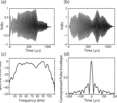
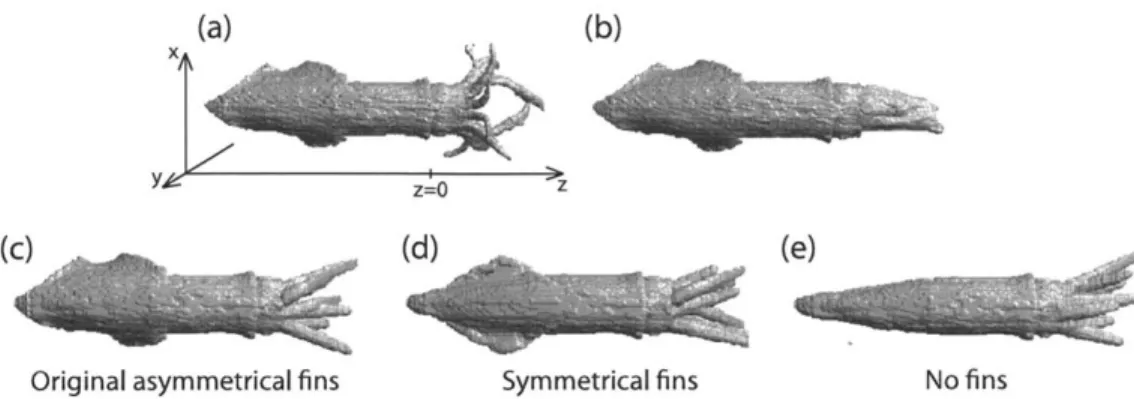
Received calibration signal. (c) Spectrum of the received calibration signal. (d) Envelope of the autocorrelation function of the received calibration signal, normalized to the peak maximum at 0 ps. . . . . . 47 2-3 Various squid shapes used in this study: (a) the arms-splayed and (b)

arms-folded squid shape without modification of the fins or random-ization of the arms. (c-e) examples of hybrid randomized squid shapes with three different shapes of the fins (see Sec. 2.3.3 for detail of the

2-4 TS prediction versus angle of orientation at four frequencies (60, 70, 85, 100 kHz) for the three-dimensional DWBA numerical model using arms-folded squid shapes with and without the fins, and the analytical DWBA prolate spheroid model. The arrow indicates the scattering contribution from the fins. . . . . 54 2-5 TS predictions versus frequency for the three-dimensional DWBA

nu-merical model using arms-folded squid shape and the analytical DWBA prolate spheroid model at four angles of orientation (00, 450 900, 1350 from normal incidence). The usable band (gray area) in the experiment lies entirely in the geometric scattering region. . . . . 55 2-6 Compressed pulse output envelope of (a) the analytical DWBA prolate

spheroid model, and the three-dimensional DWBA numerical model using two fixed squid shapes through two full rotations (7200): (b) the arms-folded configuration, and (c) the arms-splayed configuration. The compressed pulse output envelopes are normalized to the maximum envelope value in each of the plots. The symmetric sinusoidal pattern in

(a) corresponds to the front and back interface of the prolate spheroid with respect to the incidence field, and the strong sinusoidal pattern in (b) and (c) corresponds to the location of the squid arms during the rotation . . . . 57 2-7 Noise addition procedure for model predictions. (a) The frequency

de-pendent background noise profile (including reverberation) across the usable band of the experiment. (b) TS predictions with noise added

(top row) and without noise added (bottom row) based on the three-dimensional DWBA numerical model. The solid line is the mean of the measured or added noise. The gray or white area between the two dashed lines indicates the range between

+

1 standard deviation from the mean. The brackets indicate regions where the effect of noise ad-dition is more prominent. Model predictions below the noise threshold w ere om itted. . . . . 59

2-8 Temporal characteristics of the scattering at normal incidence. (a) Model predictions given by the three-dimensional DWBA numerical model with arms-folded and arms-splayed squid shapes and the ana-lytical DWBA prolate spheroid model. (b-d) Experimental data from three individuals, each with 15 individual pings overlaid at normal in-cidence. All compressed pulse output envelopes (model prediction and data) were normalized to the maximum value in each model prediction or each ping . . . . 62 2-9 Compressed pulse output envelope of (a) the experimental data from

three individuals and (b) the three-dimensional DWBA numerical model using a hybrid squid shape with randomized arms over two full rota-tions (7200). The compressed pulse output envelopes are normalized to the maximum envelope value in each of the plot. Faint vertical lines in the experimental data are due to noise not effectively eliminated by the background reverberation subtraction. . . . . 63 2-10 Data-model comparison of TS versus angle of orientation at four

fre-quencies (60, 70, 85, 100 kHz) for the individual 0822a. Hybrid

ran-domized squid shapes with three fin shapes were used in the three-dimensional DWBA numerical model: (a) original asymmetric fins, (b) artificial symmetric fins, (c) no fins. The experimental data are represented by dots. The gray area indicates the range of ±1 standard deviation from the mean of the model predictions. The arrow indi-cates the scattering contribution of the fins. The cut-off pattern near the bottom of each plot is resulted from omitting experimental data

2-11 Data-model comparison of TS versus angle of orientation at four fre-quencies (60, 70, 85, 100 kHz) for three representative individuals

(0822a, 0814a, 0819c). The hybrid randomized squid shapes with no

fins were used in the three-dimensional DWBA numerical model, with the size of the squid shape scaled to match that of each individual. The arrows indicate the potential deviation of angles of orientation during the experiment. Other details on the figure is given in the caption of

Fig. 2-10. ... ... 65 2-12 Comparison of the performance of the three-dimensional DWBA

nu-merical model and the analytical DWBA prolate spheroid model at two frequencies Frequency-dependent noise was added to both models to enable valid comparison with the data. Dots represent the ping-by-ping experimental data for the individual 0822a. The gray area indicates the range of ±1 standard deviation from the mean of the models. Note that the experimental data and model predictions lower than the background noise threshold (black lines) were not omitted in here to illustrate the difference clearly. . . . . 67 2-13 Data-model comparison of TS spectra averaged between ±20. The

angle of orientation of experimental data were adjusted by 0_adj

in cases where potential deviation in the angles of orientation were observed

(see F ig. 2-11). . . . . 68 2-14 Averaged TS versus frequency for the experimental data, the analytical

DWBA prolate spheroid model, and the three-dimensional DWBA nu-merical model using both fixed and hybrid randomized squid shapes in two planes (data only available in the lateral plane). All averages were done in the linear domain over t2 standard deviations (u) from the mean angle (pu) and converted to TS. (a) Averages in the dorsal-ventral plane. (b) Averages in the lateral plane. . . . . 70

2-15 Averaged TS versus frequency for the experimental data, the analyti-cal DWBA prolate spheroid model, and the three-dimensional DWBA numerical model using both fixed and hybrid randomized squid shapes in the lateral plane. Results from three individual squid are shown. Only a subset of models from those used in Fig. 2-14 are plotted in this figure for clarity and to facilitate inter-individual comparison. . . 71 2-16 Echo pdf of data collected within the range [750, 105') (within ±150

from normal incidence). The background noise thresholds are plot-ted for reference since all data were pooled to avoid problems in the normalization of echo pdf (see text). The figures in the left-most col-umn contain identical information as those in the second colcol-umn (data from individual 0822a) and are included to facilitate the comparison between results plotted in linear-linear and log-log axes. . . . . 75 2-17 Compressed pulse output envelopes at normal incidence for individuals

0822a and 0814a. The raw compressed output envelopes on the left show the temporal variation of the magnitude of the scattering response across pings, and the normalized compressed pulse output envelopes on the right show more detail of the temporal characteristics for each ping. The compressed pulse output envelopes on the right are normalized to the maximum value in the envelope time series of each ping. . . . . . 77 2-18 TS spectra averaged over all pings shown in Fig. 2-17. The same set

of models as those used in Fig. 2-13 are shown here for reference. . . 78 2-19 Echo pdf of data collected at normal incidence only for individuals

0822a and 0814a. Arrows indicate the narrowly-distributed echo am-plitude near the mode. Details on the figures are given in the caption to Fig. 2-16. Note that noise thresholds are not plotted in some cases when all echoes are above the threshold. . . . . 79

2-20 Echo pdf of data collected within the range [600, 1200] (within ±30'

from normal incidence). Details on the figures are given in the caption

2-21 Echo pdf of data collected within the range [300, 150'] (within t60'

from normal incidence). Details on the figures are given in the caption

to F ig. 2-16. . . . . 82 2-22 Comparison of echo pdfs of data collected within the ranges [750, 105],

[600, 1200], [300, 1500 , and [00, 360']. Details on the figures are given in the caption to Fig. 2-16. . . . . 83 2-23 Echo pdf of data collected within the range [00, 600)

U

(1200, 180c].

These echoes form a complementary set of data to those shown in Fig. 2-20. Details on the figures are given in the caption to Fig. 2-16. 84 2-24 Echo pdf of data collected measured at all angles of orientation ([0 ,3600]).

The best-fitting randomly-rough prolate spheroid models are plotted with corresponding aspect ratio (c) indicated. The model and fitting procedure are described in Sec. 2.5.2. Details on the figures are given in the caption to Fig. 2-16. . . . . 86

3-1 Illustration of analysis windows containing two possible spatial ar-rangements for aggregations composed of more than one type of scat-terer. (a) Scatterers of the same type are separated into their own subregion. (b) Scatterers of different types are uniformly interspersed throughout the analysis window. In each case, the sonar/radar resolu-tion cell is much smaller than the analysis window and, in case (a), is also much smaller than each subregion. . . . . 101 3-2 Validation of the theoretical CF-based mixed assemblage pdf using

(3.10) and (3.13) (lines) with numerically-simulated echo pdfs (sym-bols) for the case of two types of scatterers uniformly interspersed as in Fig. 3-1(b). The number of weak scatterers, N,, is fixed at 100 whereas the number of strong scatterers, N, and the ratio of the mag-nitudes of scattering amplitudes of the strong to the weak scatterers, r are both varied. . . . . 111

3-3 Comparison of echo pdfs from monotype aggregation and mixed as-semblages with varying number of scatterers and r,,. The number of dominant scatterers, Nom, is indicated for each plot. Ndom equals the total number of scatterers in monotype aggregations the number of strong scatterers in mixed assemblages (i.e., Ndom = N). N is fixed

at 100 for all mixed assemblages. . . . . 112 3-4 Variation of the CF-based mixed assemblage pdf as a function of mixed

assemblage composition. The top plots show the effect of changing N, (= 1, 5,10, 20, 50, 100) on the shape of the echo pdf when r,, = 5 and

N,, = 100. The bottom plots show the echo pdf variation with the

same combinations of N, and N., but with r,21, = 20. . . . . 113 3-5 Several representative examples of the echo pdf of simulated mixed

as-semblages (Q) and the corresponding best-fitting model pdfs (lines). Also shown on the plots are the true values of r,, and N, used to generate the simulated data. The best-fitting assemblage composition parameters for the models are summarized in Fig. 3-6. The arrows indicate the locations where the best-fitting mixture models have no-ticeable divergence from the data. . . . . 118 3-6 Comparison of the best-fitting assemblage composition parameters

ver-sus the true parameters for the CF-based mixed assemblage pdf (A), the 2-component CF-based mixture model (0), and the 2-component Rayleigh mixture model (o). The squares (0) and crosses (x) indicate the cases when the best-fitting models are composed of only one CF-based pdf component. The vertical dashed lines show the approximate locations where the performance of the CF-based mixed assemblage pdf as an inference tool starts to degrade. Note that the 2-component Rayleigh mixture model does not contain parameters N, and N,. . . 119 3-7 Comparison of CF-based mixed assemblage pdf produced with varying

3-8 Comparison of CF-based mixed assemblage pdf produced with varying rs (as shown on the legend) and fixed N. Nw is fixed at 100 for all cases... ... ... .. ... ... . . . ... . .. 121

4-1 A schematic of one realization of the numerical model showing impor-tant elements in the modeling framework. The model uses broadband signals and the echoes are processed using pulse compression before the envelopes are taken. The sample point is arbitrarily selected in the region away from the edges of the range gate, AB (= L9 in text). A

transducer with a circular aperture is used here for illustration, and can be substituted according to the specific system parameter. A low-frequency and a high-frequency narrowband beampattern (BP) are sketched to illustrate the frequency-dependent property of the beam-pattern. Note that the echoes are modulated across all frequencies according to their locations in the beam. Compared to the other two scatterers, scatterer #2 is located within the mainlobe of the beam and therefore results in a sharper echo (see Sec. 4.2.2). . . . . 131 4-2 Block diagram of the numerical simulation procedure. All involving

components are discussed in Sec. 4.2. Note the block diagram depicts the procedure to generate one realization. The ensemble of samples collected from multiple realizations is used for the estimation of the

4-3 (a) Narrowband beampatterns with respect to the polar angle (0) of a circular aperture at three frequencies (30, 50, and 70 kHz). The aperture has a radius of 0.054 m, chosen to match the specification of the high-frequency broadband echosounder used in the field exper-iment (AirMarLow channel, Sec. 4.3.1). (b) Two-way beampattern pdf [PB(b), thin black line] and the associated echo pdf produced with only one scatterer in the resolution cell [PA(a), thick black line]. Defi-nition of these quantities can be found in Sec. 3.2.3. Unless otherwise specified, the parameters of the transducer given here are used for all modeling results presented in this chapter. . . . . 135 4-4 (a) The impulse responses of the two-way beampattern at three

differ-ent polar angles (0 = 50, 10', and 30'). (b) Time domain character-istics of the autocorrelation functions of different signals modified by the beampattern impulse response. The widths of the responses are jointly determined by the bandwidths and frequency contents of the

sign als. . . . 136

4-5 Broadband echo pdf models generated with and without the beampat-tern effects in three cases with different number of scatterers (N) in the range gate. This comparison shows the strong non-Rayleigh influence of the beampattern effects. The Rayleigh distribution is plotted as a background reference for all echo pdf figures in this chapter. Unless otherwise specified, all echo pdfs in this study are normalized according to the procedure in Appendix A. . . . . 136

4-6 Spectra (a), autocorrelation functions (b), and echo pdfs (c) generated using different signals in cases with different number of scatterers in the range gate (N). Comparisons are made between: two linear chirp signals shaded using a narrow Hann window (Narrow Hann) and a wide Hann window (wide Hann); two linear chirp signals shaded using a narrow Hann window (Narrow Hann) and a wide Hann window (wide Hann); and the ideal (Ideal Tx) and actual (Actual Tx) transmit signal associated with the high-frequency broadband echosounder used in the field experim ent. . . . . 138 4-7 Comparison of echo pdf models generated using scatterers with

am-plitude distributions following the Rayleigh distribution and the dis-tribution of a randomly-rough prolate spheroid (aspect ratio ( = 5) randomly-oriented in a three-dimensional space. The influence of the strong non-Rayleigh characteristics of the scattering from the rough prolate spheroid is evident in the tail of the resultant echo pdf. . . . . 141 4-8 Comparison of echo pdf models for monotype aggregation and

two-component mixed assemblages with varying composition. The ratio between the backscattering cross section of the strong to the weak scatterers in the mixed assemblage (r,,) is varied from 5 to 30. The number of dominant scatterers in the range gate (Ndom) is defined to be equal to the number of scatterers in monotype aggregations and the number of strong scatterers in mixed assemblage, i.e., Ndom = Nw,mono = N s,mix. . . . . 143 4-9 Distribution of the length of herring concluded from trawl net catches

4-10 Calibration data and results for the three broadband channels (Shamu:

1 - 6 kHz, 424: 10 - 18 kHz, and AirMarLow: 30 - 70 kHz) channels

in the EdgeTech broadband echosounder. (a) Sphere echoes selected for use in the calibration. Each echo is plotted as a circle (Q) ac-cording to the roll and pitch angles of the towbody recorded at the instant of sonar transmission. The circles are color-coded according to the relative amplitudes of the peaks of the echo envelopes, with the red-to-blue variation denotes high-to-low amplitude variation. Circles marked with '*' are echoes with the top 5% highest amplitudes. Echoes within an arbitrarily-chosen 1.50 radius from the mean roll and pitch angles of these marked echoes (further marked by larger red circles) are selected for use in the calibration. This procedure is employed to exclude echoes resulted from off-axis insonification of the standard sphere. (b) Time-series of the envelopes of the selected echoes. Echoes from the 424 and AirMarLow channel are adjusted so that the peaks of the envelopes of specular reflections are aligned to facilitate paritial-wave analysis. Echoes from the Shamu channel are not adjusted. (c) Results of calibration for all three channels. Results for both the full-wave and partial-full-wave analyses are shown for the 424 and AirMarLow channel. . . . . 146 4-11 Examples of data and analysis of monotype (monospecific)

aggrega-tions of herring observed near the seafloor in the day time. (a) Echogram of the aggregation with two analysis windows. (b) Broadband volume backscattering strengths (Sv) and their respective best-fitting broad-band physics-based hybrid models for the two analysis windows marked in (a) (Sec. 4.4.2). Also shown are the ranges of frequency (36.3 - 39.7

kHz) included for the analysis of narrowband Sv. (c) Broadband echo pdfs of the data and best-fitting models(Sec. 4.4.1). . . . . 149

4-12 Examples of data and analysis of mixed assemblages of fish observed near the sea surface at night. (a) Echogram of the mixed assemblage with two analysis windows. (b) Broadband volume backscattering strengths (Sv) for the two analysis windows marked in (a). (c) Broad-band echo pdfs of the data. Note the prominent highly-elevated tails that may have been caused by occasional insonification of large fish in the mixed assemblage. This aggregation is the same as aggregation E that has been analyzed in Stanton et al. (2012). . . . . 150 4-13 Examples of monotype broadband echo pdf model used in the inference

analysis. The shape of the echo pdf varies from highly non-Rayleigh toward the Rayleigh distribution with increasing number of scatterers in the range gate (N). The echo pdf model's shown here are produced

with N = 10, 50, 100, 200, 500, and 800. Rayleigh-distributed noise was

added to each model following the procedure described in Appendix B. 153 4-14 (a) Two model shapes for the fish swimbladder. The first model uses

the shape of a prolate spheroid. The second model uses the cross-sectional profile of a prolate spheroid, but with its center adjusted to achieve a flat dorsal surface. The specific shapes shown here are generated assuming a swimbladder volume of 13 mL at sea surface for a 25 cm herring. (b) Examples of predicted averaged TS of this fish at a depth of 170 m evaluated using different angle of orientation distributions. The distributions of angle of orientation used here are normal distributions with different mean values (Onean=0, 50,and 100) and an identical standard deviation (Ostd = 3 . . . . . 158

4-15 Comparison of TS predictions of swimbladder resonance given by two models. The first model (Ye) was derived assuming a prolate spheroidal shape (Ye, 1997), whereas the second model (Love) assumes a spherical shape with equivalent volume (Love, 1978). The low-frequency TS predictions are plotted along with the high-frequency TS predictions given by the modal-series-based deformed cylinder model (HF) using a swimbladder shape with flat dorsal surface. The calculation uses the same parameters as in Fig. 4-14. . . . . 159 4-16 Comparison of TS predictions in the swimbladder resonance region

with different values of viscosity for fish flesh (() using Ye's model (Ye, 1997). Here, the value of ( varies from 10 to 60 Pa. s at an interval of 10 Pa. s. Calculations were made using the same parameters as in

Fig. 4-14 and Fig. 4-15. . . . . 160 4-17 (a) Echogram of the monospecific herring aggregation with analysis

windows. Windows #1 and #2 are identical to the two windows shown in Fig. 4-11. (b) Numerical density of fish estimated using various methods. Results are plotted along with their respective confidence intervals. . . . . 162

A-i Comparison of several un-normalized (top) and normalized (bottom) echo pdfs calculated using the CF-based echo pdf formula with varying numbers of only one type of scatterer (N). . . . . 188

B-i (a) Comparison of the pdfs of squid echoes and background noise, as well as their corresponding Rayleigh pdfs (see text). (c) Comparison of rough prolate spheroid echo pdf model's generated with and without

B-2 (a) Echogram of the fish aggregation with the analysis windows for fish echoes and background noise. Note that the depth of the echosounder is not corrected in this echogram so that the bottom appears to undu-late as opposed to the flat bottom shown in Fig. 4-11. (b) Comparison of the pdfs of fish echoes and background noise, as well as their corre-sponding Rayleigh pdfs (see text). (c) Comparison of broadband echo pdf model's generated with and without added noise. . . . . 192

List of Tables

2.1 Dimensions and ranges of angle of orientation for the squid used in the acoustic backscattering measurements. All dimensional measurements were conducted when the animal was dead after the acoustic experi-ment was completed. The Total Length is the length from the tip of the mantle to the tip of the arms when the squid is placed flat on a surface. The Mantle Width is the width of the widest portion of the mantle on the dorsal side. The Mantle Length is the length between the two ends of the mantle on the dorsal side. Two numbers in the Range of Angle of Orientation Measured indicate that acoustic measurements were conducted twice on the same individual. The Calculated Weight was calculated based on the published length-weight relationship for L. pealeii (Lange and Johnson, 1981). . . . . 42

4.1 Summary of model parameters used in the broadband physics-based hybrid model. Here, the ratio of specific heat, Yo, is 1.4, and D is the depth of the fish in meters. . . . . 157 4.2 Summary of potential sources of errors and corresponding impact on

the estimation results associated with model assumptions used in this study. ... ... 163

Chapter 1

Introduction

1.1

Motivation

Active remote-sensing systems acquire information by transmitting signals and re-ceiving echoes from the subject(s) of interest. One major advantage of such systems over direct on-site measurements is the ability to provide synoptic data over a large spatial scale across temporal spans relevant to the goal(s) of the study. For research fields such as oceanography and atmospheric science, such information is often de-sirable so that comprehensive understanding of the interaction among various com-ponents involved in the system can be developed (Le Chevalier, 2002; Medwin and Clay, 1998). In essence, if direct measurements of a particular quantity is considered "point samples" from its distribution, remote-sensing systems provide information that "connects the dots" through the interpretation of echoes. Another primary ad-vantage of remote-sensing systems is the ability to provide data from study sites that are difficult to access or under harsh conditions. For example, in oceanography, in-formation is often needed from locations that are remote or at great depth, and the instruments are often damaged by wind, waves, currents, corrosion, bio-fouling, pres-sure, etc. To overcome these challenges, acoustic signals, which suffer significantly less attenuation in sea water than electromagnetic signals, have been widely used to probe and characterize both the ocean interior and its boundaries (Medwin and Clay, 1998; Urick, 1983). Through evolution, similar remote-sensing techniques have also

been adopted by echolocating animals, such as bats and dolphins, for foraging and

navigation (Au, 1993; Griffin, 1958).

The study of biological oceanography is vital in understanding marine ecosystems and carries social and economic consequences as human utilization of ocean resources for food and energy have increased steadily over the past few decades (Mann and Lazier, 2005; Roberts, 2002). Basic features of biological aggregations, including taxonomic composition, patchiness of their spatial distribution, and the transient nature of their occurrence, are of fundamental importance in constructing a complete picture of biological oceanography. Such information can be collected using a variety of techniques involving the use of nets, optics, and acoustics (Harris et al., 2000). Net-based methods have been traditionally used to allow precise identification of the organisms and collection of genetic samples as well as life history data including animal length, weight, growth of gonad, etc. However, these methods suffer from problems such as net-avoidance, damage to animals, and their inherent temporal and spatial sparsity. Optical methods are capable of providing information efficiently for animal identification and behavior observation, but are limited in range and the small sampling volume due to the strong attenuation of electromagnetic wave in sea water. Contrary to the above two methods that primarily deliver point samples with sparse temporal and spatial coverage, active acoustic methods, which can provide synoptic data in high resolution across relevant temporal and spatial scales, have therefore been used extensively as a complementary survey tool in biological oceanographic

and fisheries studies (Klemas, 2012; Medwin and Clay, 1998).

However, the interpretation of acoustic echoes from marine organisms can be highly ambiguous, due to the complexity involved in the sound scattering processes. For example, the echoes are determined jointly by the properties of the transmitted signals, the propagation of sound to and from the scatterer(s), characteristics of the transmitting and receiving sensors (transducers), as well as the acoustic scattering features of the scatterer(s) (Medwin and Clay, 1998; Urick, 1983). Unique determina-tion of the sources of scattering is often difficult, and requires detailed understanding of the influences of each of the above contributing components. This research is aimed

at providing new data, models, and approaches that can serve as the basis of future development of accurate and reliable techniques for the interpretation of echoes. A brief review of the studies of acoustic scattering from marine organisms is given in the sections below, followed by an overview of the research conducted in this thesis.

1.2

Acoustic scattering from individual marine

or-ganisms

1.2.1

Principles of acoustic scattering

The acoustic scattering properties of any given object can be fully described by its complex scattering amplitude,

f,

which has both spectral and directional dependen-cies determined by the target's shape, size, angle of orientation, and material proper-ties, such as the mass density, p, and sound speed, c (Medwin and Clay, 1998). In cases where the echoes are measured in the backscattering direction, as the dynamic range of the scattered signals is typically very large, a logarithmic measure of the backscatter-ing amplitude is commonly used, defined as target strength (TS), expressed in units of decibels (dB) relative to 1 in2

, and given by TS = 10 logio Ifbs|2

= 10 log10 Ubs, where

9bs fbs 2 is the differential backscattering cross section, and fb,, or backscattering

amplitude, is the scattering amplitude evaluated in the backscattering direction. The scattering of a given object generally varies strongly as a function of frequency depending on the size of the object relative to the wavelength (Medwin and Clay, 1998). This functional dependency can be understood by comparing the acoustic wavelength (A) to the characteristic dimension of the object (a, such as the radius for spherical object or the length of elongated objects) through the dimensionless quanti-ties ka, where k is the acoustic wavenumber, defined by k = 27r/A. The ka

<

1 case is usually referred to as the "Rayleigh scattering region", where the wavelength is much larger than the object and the backscattering cross section is generally proportional to (ka)" for objects without gas inclusion. When ka

>>

1, the acoustic waves can be approximated as "rays" in this "geometrical region", and the scattering occurs at the

discontinuities within and at the boundaries of the object (Medwin and Clay, 1998). In the intermediate region, however, the scattering characteristics are complex and contain prominent structures, such as resonances, depending on the detailed physical properties of the target (Ainslie and Leighton, 2011).

For objects with simple geometry and internal structure, such as spheres and spherical shells, the exact scattering functions can be derived analytically and used for benchmark assessment for the scattering from more complex objects or verification of other approximate solutions. The scattering functions can be obtained by solving the Helmholtz-Kirchhoff integral over the object boundary, or by expanding the solutions to the wave equations in convenient coordinate systems, and matching the boundary conditions at the interface of the scatterer and the medium. In the latter case, the scattering function can be understood as a series of "modes" supported by the particular geometry and material properties of the object. For example, the dominant resonance of a gaseous body in the ka

<

1 region is trackable through the lowest mode in the modal-series solution, while the inclusion of higher modes gives a complete description for the scattering across all ranges of ka.

Although marine organisms are generally of much more complex outer shapes and internal composition, studies of the acoustic scattering properties of simple objects bring important insights that can be applied to understand the scattering from marine organisms, as will be seen in the next section.

1.2.2

Scattering models

Quantitative interpretation of echoes for biologically-relevant information requires de-tailed knowledge on the acoustic scattering characteristics of different types of marine organisms. Better understanding and modeling capabilities for the scattering from individual animals form the basis for accurate interpretation of echoes collected in the field (Medwin and Clay, 1998). Despite the often complex shape and internal structure of animal bodies, the acoustic scattering properties of marine organisms can generally be determined according to their gross anatomical features and mate-rial properties of important organs, with additional modification due to

individual-or behaviindividual-or-related characteristics. Such infindividual-ormation is usually obtained using labo-ratory experiments with individual animal fixed on the main axis of the transducer and insonified at a designated set of angles of orientation in the far-fields of both the transducer(s) and the animal (Stanton, 2012). This setup allows direct observation of the scattering features from the animal, which are are useful for the development and verification of scattering models of individual animals. The following sections discuss the modeling of the acoustic scattering of three representative groups of ma-rine organisms categorized according to their gross anatomical features: fluidlike, elastic-shelled, and gas-bearing (Stanton et al., 1998a,b). These three categories were established from studies on the scattering from fish and zooplankton, and can be extended to include other animals with similar anatomical features.

The fluidlike animals are represented by euphausiids, copepods, and decapod shrimps, whose bodies are composed primarily of weakly-scattering materials with sound speed and density very close to those of the sea water. The boundary of the an-imal behaves acoustically as a fluid-fluid interface and does not support shear waves. These properties prompt the use of a series of models incorporating the weakly-scattering material properties with increasingly complicated representation of the shape of the animal, including a modal-series-based line integral or a ray summation using a deformed cylinder formulation (Stanton, 1989; Stanton et al., 1993b), and a distorted-wave Born approximation (DWBA) formulation in which the scattering is evaluated by a volume integral (Chu et al., 1993; Morse and Ingard, 1987; Stanton

et al., 1998a, 1993a). For fluidlike scatterers with elongated shapes, such as that of

euphausiids, the scattering can be qualitatively described by two rays from the front and back interfaces between the animal body and the medium at normal incidence, and the scattering across all angles of orientation can be predicted using more sophis-ticated model that includes roughness and inhomogeneity within the body (Lavery

et al., 2002; Stanton et al., 1998a). These dependencies have been verified by various

experiments conducted both in the laboratory and in the field (Lawson et al., 2006; Stanton et al., 1998b).

char-acterized by their possession of a hard elastic shell (Stanton et al., 1998a,b). The scattering is dominated by the dense elastic shell which gives rise to a series of highly complicated echoes from the specular reflection of the front interface, internal refrac-tion and reflecrefrac-tions within the the shell and the body, and a class of circumferential waves propagating on the shell and the immediate surrounding fluid (Stanton et al.,

1998a). Although such decomposition of different scattering components can provide physical insights to the scattering mechanisms of these animals, the complexity of the boundary and shape of the elastic shell is challenging, and numerical evaluation of the wave equation or generalized ray theory is usually necessary for exact modeling of their scattering functions (e.g., Jansson, 1993; Kargl and Marston, 1989; Marston

et al., 1990; Rebinsky and Norris, 1995).

The third category of animals is characterized by the inclusion of gas in their body (gas-bearing), such as fish with swimbladders and siphonophores possessing pneumatophores. Due to the large contrast between the air and seawater, the gas in-clusion dominates the scattering from this type of animal, and features in the echoes can be explained by identifying the contributions from the gas bubble and the re-maining fluidlike body or bony structure, if present (Foote, 1985; Reeder et al., 2004; Stanton et al., 1998a,b; Sun et al., 1985). Due the complexity involved, the scatter-ing from gas-bearscatter-ing animals is generally predicted usscatter-ing hybrid models consistscatter-ing of separate models for different scattering regimes (Chu et al., 2006; Clay and Horne,

1994; Jech and Horne, 2002; Stanton et al., 2010).

For the scattering from the gas-bearing organ, when ka < 1, the breathing mode

dominates the scattering with an omnidirectional scattering pattern and a resonance behavior determined by the volume and associated damping parameters (reradia-tion, thermal, and viscous damping (Ainslie and Leighton, 2011; Medwin and Clay,

1998). Models are usually derived by solving for the scattering pressure from the

wave equation using simple geometries, such as spheres or prolate spheroids (Feuil-lade and Nero, 1998; Love, 1978; Ye, 1997; Ye and Hoskinson, 1998), with appropriate boundary conditions and volumes equivalent to those of the gas-bearing organs. In the ka > 1 region, on the other hand, the scattering becomes highly directional and

is determined by the exact shape and orientation of the gas inclusion with respect to the incidence waves. The scattering in this region has been modeled by the co-herent summation of a series of objects with simple geometries that jointly capture the shape of the gas-bearing organ. Examples include the Kirchhoff ray-mode model which approximates the swimbladder morphology by a series of finite-length cylinders (Clay and Horne, 1994; Jech and Horne, 2002), and the modal-series-based deformed cylinder model which evaluates the scattering through a line integral over circular slices with variable radius along an arbitrary center line (Stanton, 1989; Stanton

et al., 2010). Another class of models often incorporates the complex outer shape

of the swimbladder and uses sophisticated numerical methods such as the boundary-element method to predict its scattering features (Foote and Francis, 2002; Francis and Foote, 2003). The scattering from the soft body is generally predicted using mod-els consistent with the fluidlike material properties of the tissues, such the DWBA model, or modal-series-based deformed cylinder model and the Kirchhoff-ray model solved with fluidlike boundary conditions.

Although the scattering contributions from the gas-bearing organ and the body tissues add coherently to form the scattering from the whole animal, in practice these two components are usually summed incoherently to model the scattering from the whole animal. This operation is justified by the relatively weak contribution from the soft tissue and the smearing of the exact phase information due to the complicated

morphology of the animals (Gorska and Ona, 2003b).

There remain unanswered questions in our understanding of the acoustic scat-tering from the above organisms. For example, as important as the swimbladder is in determining the scattering from fish, the depth-dependency of its geometry with respect to the behavior and life history stage of fish remains unclear (Diachok, 2005;

Fissler et al., 2009b; Gorska and Ona, 2003b; Horne et al., 2009; Ona, 1990). This

question is further complicated by the diversity in the anatomical features of fish swimbladders, among them the differences between physostomes (fish with a swim-bladder connected to the stomach through a pneumatic duct) and physoclits (fish with a closed swimbladder) (as reviewed in Diachok, 2005). Furthermore, although

key factors influencing the scattering of individual organisms, such as the distribution of the length, angle of orientation, depth, etc., have been identified in the models, the relative importance of each factor on the scattering, as well as the variability of these parameters needs to be quantified systematically in a biologically-meaningful context (Hazen and Horne, 2003; Lawson et al., 2006).

Although the models introduced above were derived based on the physical proper-ties of zooplankton and fish, their application may be extended to predict the scatter-ing from other animals with similar anatomical features and material properties. For example, the class of models developed for fluidlike zooplankton have been applied to predict the scattering from a variety of animals with fluidlike, weakly-scattering material properties, such as squid, fish without swimbladders, and other gelatinous zooplankton (Brierley et al., 2004; Jones et al., 2009; Kang et al., 2006; Warren and

Smith, 2007; Wiebe et al., 2010; Yasuma et al., 2010, 2006). However, direct

appli-cation of existing models should be treated with caution, since the scattering from any given animal may be strongly influenced by taxon-specific organs or structures. Therefore, it is important that dominant scattering mechanisms of different animals be identified through experiments, and detailed data-model comparison be conducted to assess the performance of existing models and guide further model development.

1.3

Measurement and analysis of in-situ echo

1.3.1

Echo measurements in field experiments

Active acoustic survey techniques infer biologically-relevant information through fea-tures in the scattered signals. Depending on the experimental scenario, acoustic scattering measurements can be categorized into three groups: monostatic, bistatic, and multistatic, according to the geometry among the transmitter, receiver, and scatterers (Medwin and Clay, 1998). The transmitters and receivers are spatially col-located for monostatic systems and are separated for the other two types of systems. Bistatic measurements refer to the scenarios in which there is one pair of spatially

separated transmitter and receiver, while multistatic systems often involve multiple sets of spatially diverse monostatic or bistatic sensors. Most acoustic scattering stud-ies of marine organisms are conducted using monostatic systems, and therefore the modeling and analysis generally focus on echoes received in the backscattering direc-tion. Notable exceptions are theoretical studies and experimental works on forward scattering from the swimbladders of fish (Diachok, 1999; Ding, 1997; Ye and Farmer, 1996).

To the contrary of the scenarios in laboratory experiments, acoustic scattering measurements of marine organisms in the field usually involve one or multiple un-controlled scatterers in the sampling volume (Foote, 1991; Medwin and Clay, 1998). In this case, characteristics of the sensing system and transducer beampattern, the locations of the organisms in the beam, and the scattering properties of each individ-ual organism jointly determine the echo signals received on the sensing system and have to be taken into account for accurate interpretation of echoes. "Echograms", or compilations of echo time-series from multiple insonifications of the same scatterer or sets of scatterers, reveal volumes with high-amplitude echo returns and are usually used to guide the focus of echo analysis. Conventional acoustic scattering researches, especially the studies of fish aggregations, rely heavily on subjective description of morphological characteristics of aggregations on the echograms, but more quantitative and objective echo analysis methods have been adopted in recent studies to make use of acoustic information embedded in the echoes (Jech and Michaels, 2006; Simmonds and MacLennan, 2006).

Sensing systems used in field experiments can also be categorized according to the directions in which the signals are transmitted and received. Downward-looking echosounders are standard systems used in fisheries applications and usually involve higher frequency signals at 10's to 100's kHz for the observation of individuals or aggregations of organisms located directly below the echosounders (Simmonds and MacLennan, 2006). Horizontally-looking systems are generally developed for research purposes and use signals at the range of 100's Hz to 10's kHz for collecting synoptic data of biological aggregations across a large area (Farmer et al., 1999; Gauss et al.,

2009; Jones and Jackson, 2009; Makris et al., 2006; Revie et al., 1990; Rusby et al., 1973; Trevorrow and Pedersen, 2000). These two types of system differ primarily

in the propagation paths of the transmitted and scattered signals, where direct-path propagation between the transducers and scatterers are expected for most downward-looking echosounders, and waveguide modulation results from ocean boundaries, such as the sea surface and seafloor, is important for horizontally-looking echosounders. Stanton (2012) provides a brief discussion on the pros and cons of each of these systems.

The sections below review common techniques used for the analysis of in-situ echoes collected using downward-looking, monostatic systems that are typical for

acoustic scattering studies of marine organisms.

1.3.2

Echoes from individual marine organisms

When the numerical density of organisms is low and the number of organisms in each sonar resolution cell is less than one, direct measurement of the backscattering from individual animals is possible by properly thresholding of the echo time-series [often referred to as "echo counting", (Medwin and Clay, 1998)]. Different from the situation in controlled laboratory experiment in which the experimental animal is located on the main axis of the transducer, the amplitudes of echoes from organisms in the field are modified depending on its location in the sonar beam. This beampattern modulation has to be removed to recover the actual echoes from the organisms. The beampattern effects can be eliminated through direct methods in which the target location in the beam is inferred by comparing the amplitudes and phases of signals received on separate sector of dual-beam or split-beam transducers, so that the scaling factor can be calculated and corrected (Ehrenberg, 1989). In cases where single-beam transducers are used, the distribution of the actual echoes from the targets can be obtained by indirect methods that utilize deconvolution, inversion, or iterative procedures to eliminate the influence of the beam pattern (Ehrenberg, 1989; Fissler

et al., 2009a; Stepnowski and Moszynski, 2000).