Autonomous and Adaptive Underwater Plume Detection and
Tracking with AUVs: Concepts, Methods, and Available Technology
The MIT Faculty has made this article openly available.
Please share
how this access benefits you. Your story matters.
Citation
Petillo, Stephanie M., and Henrik Schmidt. “Autonomous and
Adaptive Underwater Plume Detection and Tracking with AUVs:
Concepts, Methods, and Available Technology.” IFAC Proceedings
Volumes 45, 27 (2012): 232–237 © IFAC
As Published
http://dx.doi.org/10.3182/20120919-3-IT-2046.00040
Publisher
Elsevier BV
Version
Author's final manuscript
Citable link
http://hdl.handle.net/1721.1/114874
Terms of Use
Creative Commons Attribution-NonCommercial-NoDerivs License
Autonomous and Adaptive Underwater
Plume Detection and Tracking with AUVs:
Concepts, Methods, and Available
Technology ⋆
Stephanie M. Petillo∗Henrik Schmidt∗∗
∗Massachusetts Institute of Technology, Cambridge, MA 02139 USA,
& Woods Hole Oceanographic Institution, Woods Hole, MA 02543 USA (e-mail: [email protected])
∗∗Massachusetts Institute of Technology, Cambridge, MA 02139 USA
(e-mail: [email protected])
Abstract: An autonomous underwater vehicle (AUV) equipped with environmental sensors and an on-board autonomy system can greatly increase the efficiency of environmental data collection and the synopticity of the data set collected simply by autonomously adapting its motion to changes it senses in its local environment. One application of this is tracking ocean features in an unknown ocean environment. This can be accomplished with one or multiple AUVs collaborating in near-real-time using acoustic communications. To further explore one example of this application, this paper focuses on using multiple AUVs to track underwater plumes. We evaluate various types of plumes (e.g., hydrothermal vent plumes, algal blooms, oil leaks), how each plume type may be detected and its spatial extent determined, what types of sensors can be used, and how AUVs can be employed to autonomously and adaptively track these dynamic plumes. Since AUVs vary significantly in design, mobility, deployment duration, on-board processing power, etc., it is also necessary to consider the best choice of AUV (or combination of AUVs) to track a plume. Thus, an operator/scientist’s choice of AUV type(s) will likely depend the type of plume to be tracked, or vice versa. Since most underwater plumes are highly spatiotemporally dynamic, employing environmentally adaptive autonomy to track them with a fleet of AUVs is one of the most efficient ways to do so, given today’s technology.
Keywords: Autonomous vehicles, Adaptive systems, Marine systems, Sampling systems,
Tracking applications, Marine environmental sampling, Underwater plumes 1. INTRODUCTION
The ability to detect and track underwater plumes in an ever more efficient manner is relevant to both scientists and civilians alike. These underwater plumes may be in the form of hydrothermal vent plumes found deep in the ocean, oil spills which may be far out at sea or near coasts or fishing grounds, harmful algal blooms (HABs) that cause beach closures and make exposed shellfish toxic to humans, river outflow plumes of chemicals or suspended sediment, plumes of tracer dye, etc. Each type of plume has specific physical, chemical, and biological properties, as well as characteristic spatial and temporal scales over which the plume’s area of coverage changes significantly. Dynamic ocean features such as these are best sampled from a variety of perspectives (using complimentary sensor measurements and/or taking measurements from different positions inside or outside of the plume), of which a few approaches are described in Camilli et al. (2010); Smith et al. (2010); Das et al. (2010); Jakuba et al. (2005); Petillo
⋆ Financial support of this work was provided by the U.S. Office of Naval Research (award # N000141110097) GOATS‘11 project -Adaptive and Collaborative Exploitation of 3-Dimensional Environ-mental Acoustics in Distributed Undersea Networks.
et al. (2012); Farrell et al. (2005); Pang and Farrell (2006); Pang (2010); Cannell et al. (2006).
The plume detection and tracking techniques described in the aforementioned papers have the common approach of using AUVs to complete the bulk of the plume sampling, employing autonomous plume detection and tracking al-gorithms on-board the AUVs when possible. However, for each group, a different type of AUV is used to detect and track a different type of plume using different autonomy algorithms. These differences make it difficult to compare the individual approaches to plume tracking. Thus, we propose to evaluate a variety of AUVs based on their capabilities (design, mobility, deployment duration, on-board processing power, etc.) in an attempt to find an optimal plume-to-AUV match.
Finally, we will discuss the various autonomous and adap-tive plume detection and tracking techniques that have been tested and suggest a system of our own involving the use of a fleet of autonomously collaborating AUVs that communicate in near-real-time using acoustic transmis-sions and adapt their motion to changes in the environ-ment to best detect and track a plume. Here we will also account for the fact that, depending on plume type, the
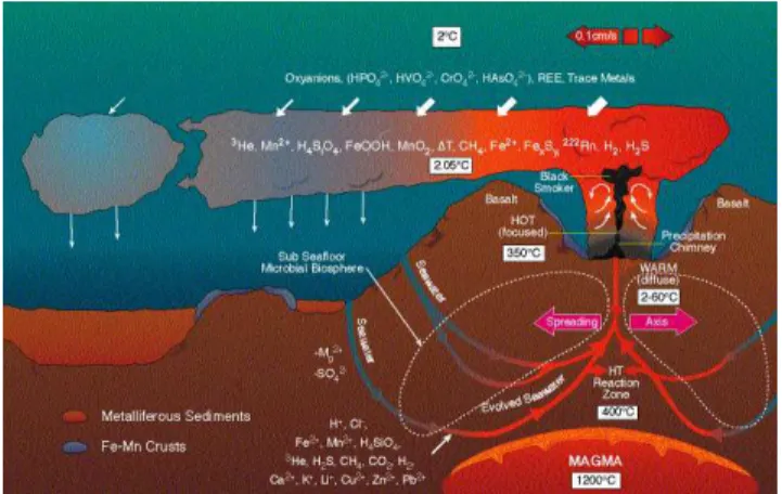
Fig. 1. Formation of a hydrothermal vent plume. Image credit: National Oceanic and Atmospheric Adminis-tration’s Pacific Marine Environmental Laboratory (b).
AUV(s) will be either looking for the approximately 2-D spatial boundary of the plume’s non-buoyant layer in the horizontal plane, or for the plume’s source location.
2. PLUMES
Plumes are dynamic features that evolve over space and time. Below we describe three prominent types of plumes, how they form, how they are characterized, and how we can detect them using AUV-mounted sensors.
2.1 Hydrothermal Vent Plumes
Hydrothermal vents occur on the sea floor at circulation zones near underwater plate boundaries, most often along plate spreading centers. In these regions, seawater seeps down into the earth’s crust, undergoing chemical reactions as it is rapidly heated within the rock below before it is ejected back up through a sea floor hydrothermal vent and into the cold surrounding seawater. This chemical-filled vent fluid rises, reacts with its surrounding environment, cools, mixes, and spreads out horizontally at some distance above the sea floor to form a hydrothermal vent plume. This process is depicted in Fig. 1.
Hydrothermal vent plumes are characterized by the spatial extent of a plume’s non-buoyant layer above the sea floor, which, according to Baker et al. (1995), can extend tens to thousands of kilometers from the vent itself. Thus far, the most successful way to find the source of a hydrothermal vent plume is to first find the plume, and then track its chemical and physical signature back to its source. In particular, scientists examine temperature anomaly, particle content, water velocity, chemical tracers (iron, manganese, helium, methane, hydrogen sulfide), and bathymetric signatures in the water near potential hydrothermal vent sites to determine the presence of a plume and vent field.
A number of sensors that detect the aforementioned chem-ical and physchem-ical signatures are given in table 1 (see Na-tional Oceanic and Atmospheric Administration’s Pacific Marine Environmental Laboratory (a) and Conrad (2008) for further sensor details). Many of these sensors can be
mounted off-the-shelf onto an AUV, although some are still custom-made for oceanographic applications.
Table 1. Sensors to detect hydrothermal vent plumes and sources
Signature Sensors
Temperature anomaly CTD
(Conductivity-Temperature-Depth) sensor
Particle content Optical sensors: transmissometer,
nephelometer
Water velocity Acoustic sensors: ADCP (Acoustic Doppler
Current Profiler), sidescan sonar, multibeam sonar
Chemical tracers Optical sensors: SUAVE (System Used to
Assess Vented Emissions), ZAPS (Zero Angle Photon Spectrophotometer),
eH (redox potential) sensor
Bathymetry Multibeam mapping sonar, camera
(still or video)
2.2 Oil Spills
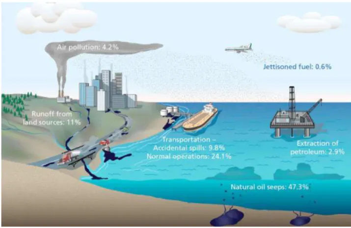
There are two primary sources of oil input into the ocean: natural seeps from beneath the sea floor that account for about 50% of oil in the coastal ocean and oil spills (and oil runoff) from human activities (see Fig. 2). Since the methods for detecting oil seeps are not within the scope of this paper, we address only oil spill characteristics here. When an oil spill results from human activities, the source location is often well known, and scientists need to know the spatial extent of the resulting oil plume in order to assess damage to the environment, flora, fauna, ocean-sourced food supplies, and coastal human populations. Although a large portion of oil rises to the surface during a spill event to form a slick, over time (on the order of seconds to years) the chemicals in oil react with the seawater and are consumed and broken down by microbes in the water, leading to an eventual fallout of the remains of the oil into a layer in which it is neutrally buoyant and/or into a pile on the sea floor, where microbes in the sediment further break down the oil. As evidenced in the work of Camilli et al. (2010), a significant amount of oil may be entrained in a neutrally buoyant layer well below the sea surface long after the surface slick has been dispersed and before total fallout occurs.
Oil spills vary widely in horizontal extent depending on the type of source supply (e.g., ship leak, broken well pipe on a drilling rig, shore runoff, etc.) and local flow characteristics. The underwater plume from the leaking MC252 Macondo well site in the Gulf of Mexico, for example, exhibited 5-day-old oil that had spread over 30 kilometers from the well head location when the team of Camilli et al. (2010) found and mapped the plume. The residence time associated with oil in the ocean can vary from months to years, depending on the severity of the spill/leak. Seep oil in particular remains on the surface or suspended in the water column for anywhere from about 10 hours to 5 days before settling to the sea floor (see Woods Hole Oceanographic Institution (2011)). Thus, a similar time line is likely for some oil resulting from spills.
Fig. 2. Sources of oil in the ocean. Image credit: Jack Cook, Woods Hole Oceanographic Institution (2011). Finally, the best way to detect the presence of oil in the water is to analyze the hydrocarbon concentration of the water. There are a number of sensors that have been used to detect hydrocarbons in the water remotely, in a lab, and in situ. Mazumder and Saha (2006) have used thermal infrared sensors, laser fluorosensors, and radar to sense hy-drocarbon concentration. Other techniques involve ADCP or Doppler Velocity Log sensors to record the currents and predict spreading direction of the oil, while a mass spectrometer is used to detect the hydrocarbons.
2.3 Harmful Algal Blooms
Harmful algal blooms differ from hydrothermal vent plumes and oil seeps and spills in that HABs do not have a source location feeding the plume (bloom). Instead, HABs are triggered when significant amounts of nutrients (nitro-gen and phosphorous) and light are sustained in a region, resulting in an abundance of algal growth (blooming) that is often visible by the human eye as tiny red, green, orange, or brown particles (algae) floating in a thick layer near the surface of the water. Such areas are often classified as eutrophic zones along the coast, since nutrient runoff from land usage gets trapped in the relatively shallow and warm coastal waters, resulting in algal blooms. In such high concentrations, the toxins in some types of algae become lethal to marine organisms that consume them (and to people that eat the contaminated seafood), and can even result in a hypoxic zone due to the depletion of dissolved oxygen by the excess of algae.
Since HABs do not have a source, once the bloom is formed, it is transported largely by physical ocean pro-cesses such as coastal currents, wind, buoyancy, mixing, tides, and eddies. This transport can carry the bloom hundreds to thousands of kilometers. The vertical extent of the bloom is often on the order of tens if centimeters, making it a nearly 2-D feature in space, spreading out horizontally near the surface or along the thermocline, covering 10-1000 kilometers in range (see Glibert (2006)). The residence time of a given HAB varies widely based on nutrients, light, and algal life cycle.
There are a number of ways to detect and classify algae in a HAB, some of which are in situ, and some must be used on samples in a lab (see Glibert (2006)). In situ sensors for HAB detection:
• Nutrient monitors
• Antibody probes (for a phosphorous-regulated pro-tein)
• Flow cytometry
• Chlorophyll in vivo fluorescence (not ideal, as not all HABs contain chlorophyll)
• Nucleotide probes
• Quantitative polymerase chain reaction (PCR) Other sensors for HAB detection:
• Microarray chip technology
• Electrospray ionization mass spectrometry
• Visual microscopic examination of water/biomass samples (a slow and tedious process)
3. AUVS
Having classified the primary plume types that we would like to detect and track with AUVs, we now move on to classify the abilities and traits of a variety of AUVs. Although this will not be a thorough classification of all AUVs, since there are many different commercial and made-in-house AUVs in the ocean community today, we aim to generalize a number of AUVs into categories that will allow us to best select a type of AUV to track a specific type of plume.
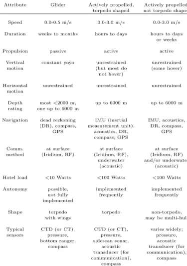
The most basic attributes to look at when compar-ing AUVs are speed, deployment duration (battery life), propulsion (active or passive), range of motion control, depth rating, navigation method, communication, hotel power load on board, autonomy system, hull shape, ease of retrofitting sensors, and what sensors it carries ‘off the shelf’. See table 2.
Some examples of the AUVs that fall into the three categories in table 2 are listed below.
Gliders:
• Slocum gliders (thermal and electric) from Teledyne Webb Research
• Spray gliders from Bluefin Robotics • ANT Littoral gliders from ANT, LLC.
• Seagliders from iRobot and the University of Wash-ington
Actively propelled, torpedo shaped AUVs:
• Bluefin 9”, 12”, and 21” from Bluefin Robotics • Ocean Explorer (OEX) from the NATO Undersea
Research Centre, Italy
• REMUS from Hydroid-Kongsberg Maritime • Iver from Ocean Server
• Folaga from Graal Tech (more like a hybrid glider-but-actively-actuated, torpedo-shaped AUV)
Actively propelled, not torpedo shaped AUVs:
• Sentry and Autonomous Benthic Explorer (ABE) from Woods Hole Oceanographic Institution (WHOI) • Puma, Jaguar, and SeaBED-class from WHOI • Odyssey IV Class from Massachusetts Institute of
Technology’s Sea Grant AUV Laboratory
To pair AUVs with a type of plume it is best suited to detect or track, we will consider the two primary classifications of AUVs: gliders and actively propelled
AUVs. For long-duration deployments (days to months), the duration of gliders makes them the best type of AUV for the job. Multiple gliders distributed in a coordinated manner are also marginally sufficient to track a HAB advected by ocean currents, since the passive propulsion and resulting slow speed of gliders through the water are directly affected by the currents as well, pushing the gliders in the same direction as the plume is advected (see Smith et al. (2010); Das et al. (2010)). For very deep missions that are time-dependent (achievable in or requiring short mission time, as in hours or days), involve plumes that are highly time-variant, or require tracking a plume to its source against the local currents, actively propelled AUVs are the better choice despite their shorter deployment duration. This includes quickly detecting, tracking, and mapping an oil spill plume as in Camilli et al. (2010), as well as searching for hydrothermal vents near the sea floor while the plume changes location due to deep currents as experienced by Jakuba et al. (2005). In these cases, actively propelled AUVs may be used solo, or in a coordinated fleet if a meso- or large-scale plume must be mapped as the plume advects with the changing currents. Actively propelled AUVs would also be useful in quickly surveying the plume extent of a HAB in the horizontal plane, providing more of a snapshot of the HAB position as the AUV(s) is(are) deployed from day to day (and retrieved to recharge overnight).
Table 2. Attributes of various types of AUVs
Attribute Glider Actively propelled, Actively propelled,
torpedo shaped not torpedo shaped
Speed 0.0-0.5 m/s 0.0-3.0 m/s 0.0-3.0 m/s
Duration weeks to months hours to days hours to days
or weeks
Propulsion passive active active
Vertical constant yoyo unrestrained unrestrained
motion (but most do (some hover)
not hover)
Horizontal unrestrained unrestrained unrestrained
motion
Depth most <2000 m, up to 6000 m up to 6000 m
rating one up to 6000 m
Navigation dead reckoning IMU (inertial IMU, acoustics,
(DR), compass, measurement unit), DR, compass,
GPS acoustics, DR, GPS
compass, GPS
Comm. at surface at surface at surface
method (Iridium, RF) (Iridium, RF), (Iridium, RF)
underwater and/or underwater
(acoustic) (acoustic)
Hotel load <10 Watts <100 Watts <100 Watts
Autonomy possible, implemented implemented
not fully frequently frequently
implemented
Shape torpedo torpedo non-torpedo,
with wings may be multi-hull
Typical CTD (or CT), CTD (or CT), varies widely;
sensors pressure, pressure, pressure,
bottom ranger, sidescan sonar, acoustic
compass acoustic transducer (for
transducer (for communication),
communication), compass
compass
4. PLUME TRACKING METHODS
With a knowledge of the capabilities of various AUVs and the characteristics of underwater plumes, there are a variety of approaches to take towards autonomously and adaptively detecting and tracking plumes with AUVs. Here we will look at the plume detection and tracking methods of a number groups and present the preliminary methods proposed by our group.
4.1 Related Literature
Tracking the general motion of HABs with AUVs (gliders, in particular) has been explored by Smith et al. (2010) and Das et al. (2010). Smith et al. (2010) used a regional ocean model off of the coast of California to forecast the advection of an imaginary HAB that is tagged by actual Lagrangian drifters in the region, while Das et al. (2010) look for “hotspots” of high-concentration HAB patches using satellite and high-frequency radar data sets. Both use the frequently-updated remote sensing information and in-water drifter positions to tag the HABs, and then run mission-planning algorithms on a shore- or ship-side computer to update waypoint paths every few hours for gliders deployed in the area to actively track the (imaginary) HAB as it advects. Although these are good approaches to HAB tracking, the use of remotely sensed data or models requires extra time, computational power, and hard drive storage space that is not available on board gliders, and often not available on actively-propelled AUVs either, requiring connection of the AUVs to some shore- or ship-side computer to update the models and AUV paths. The works of Farrell et al. (2005) and Pang and Farrell (2006) are very significant to this field, as they employ actively-propelled AUVs to detect and track man-made plumes of Rhodamine dye back to their sources in a rela-tively constant flow field within the bottom boundary layer of coastal waters (<30 meters deep). The REMUS AUV used by the group in field experiments was equipped with an ADCP unit to record the currents through the water column, a sensor that could detect trace concentrations of the Rhodamine dye for tracking the plume, and on board autonomy algorithms that perform lawnmower pattern surveys in the horizontal plane at constant altitude above the sea floor until the sensors detect the dye plume, at which point the AUV switches autonomously into plume-tracking mode. In plume-plume-tracking mode, it uses a com-bination of real-time current data and dye concentration data it has collected to determine the direction of travel with the highest probability of finding the dye source, zig-zagging across the plume in the horizontal plane until it has determined the source location. Pang (2010) takes this one step farther using Artificial Potential Field methods in simulation to improve upon source localization algorithms with the application of tracking hydrothermal vent plumes to find the vent locations.
The work by Jakuba et al. (2005) takes a somewhat dif-ferent approach using a towed instrument package with a CTD and optical backscatter (OBS) sensor to detect the non-buoyant plume emitted from hydrothermal vents at the Juan de Fuca Ridge, and then deploying WHOI’s ABE AUV to localize the hydrothermal vents. The vent localiza-tion was done as nested lawnmower surveys of successively
finer resolution using a combination of eH, temperature, depth, and OBS sensors, multibeam bathymetric mapping, and photos for creating photomosaics of the sea floor vent sites. The increased efficiency that would result from automating the nested surveys and incorporating current measurements into vent localization is also discussed in the paper, though these improvements had not been fully implemented at the time of writing.
Camilli et al. (2010) took a reconfigurable, but not au-tonomous, zig-zagging plume tracking approach to detect and track the path of the underwater oil plume from the leaking Macondo well in the Gulf of Mexico using WHOI’s Sentry AUV. Sentry’s mass spectrometer gathered hydro-carbon concentration data along its path, sending snip-pets of data via acoustics back to the shipboard AUV operator for inspection in case the AUV mission needed reconfiguring to keep the vehicle in contact with the plume. Towed instruments and instruments cast over the side of the ship to collect further data and water samples also provided data to augment and verify the data collected by Sentry. This is one example in which, if more on board AUV autonomy were employed to adapt the AUV’s motion to its sensor readings, much mission planning and AUV redirection on the part of the AUV operators and scientific crew could have been eliminated, and AUV excursions kilometers from the plume could have been significantly reduced, saving time and battery power.
Finally, Cannell et al. (2006) proved autonomous and adaptive plume mapping and boundary tracking possible using a single AUV to map the outflow plume of cool-ing water from a nuclear power plant. The AUV could adaptively zig-zag across the plume and along the plume boundary.
4.2 Our Approach
We propose to employ a behavior-based autonomy ar-chitecture on board AUVs (both actively-propelled and gliders) in order to make the adaptation of the AUVs’ motions to the environment fully autonomous. Preliminary testing of autonomous and adaptive environmental feature tracking has already been successfully completed on a number of models of actively propelled AUVs (see Petillo et al. (2010)), but the power restrictions on board gliders have prevented the use of fully on-board autonomy thus far. A number of groups (including ours) are currently looking into this problem, and we expect to see some fully autonomous gliders tested in the next few years as more autonomy systems migrate onto low-power embed-ded computers.
It is easiest to attempt plume tracking with a single AUV due to the relative simplicity of deploying and monitoring only one vehicle; however, it may be physically impossible to collect a synoptic data set representing a meso- or large-scale plume with only one AUV due to speed, battery life, and other constraints. On the meso- and large- horizontal spatial scales (tens to hundreds of kilometers, or more) frequently covered by dynamic underwater plumes, it is reasonable to assume that the use of multiple AUVs with the ability to autonomously coordinate their own motions through acoustic (or radio-frequency, if absolutely neces-sary) communication methods would be advantageous.
With fully autonomously-controlled AUVs in mind (both solo and coordinated in a network), we discuss various approaches to tracking plumes with different character-istics below. We assume that non-buoyant plume layers can be approximated as 2-D when plume tracking in the horizontal plane.
Non-buoyant layer plume detection. The search for a non-buoyant layer plume consists of motion in the horizon-tal plane coupled with depth excursions along the vertical axis. The vertical motion is a yo-yo pattern to determine the depth range in which the non-buoyant plume is float-ing. This allows all types of AUVs (gliders and otherwise) to be suited to this task. The horizontal motion of an AUV may be a circular pattern centered around the source location (if known) to determine the dominant direction that the plume has spread in, or it may be a rectangle, strait line, or lawnmower survey pattern over an area where sources are predicted to be nearby (or if there is no source, as in a HAB) in hopes of detecting a plume.
Plume source discovery. To find an unknown source lo-cation after a plume is detected, detect and track the non-buoyant plume back to its source. There are a number of approaches to this which are best suited to actively pro-pelled AUVs, with the ability to make headway swimming against the currents and easily change heading if necessary. Gliders are much slower to travel and maneuver, with a maximum speed through water of under 0.5 m/s (and often <0.3 m/s), making little or negative headway against currents any greater than about 0.5 m/s.
Assuming an AUV has a current measuring device such as an ADCP on board, once the plume is detected, the AUV may attempt to swim directly upstream against the current towards the presumed source location. However, it is likely that the plume’s meandering motion from time-dynamic currents results in an indirect path back to the source, requiring the AUV to perform a horizontal zig-zagging motion to remain in contact with the plume as it follows the plume upstream. If the plume is relatively skinny, O(1 km), and the currents are largely constant in direction, as in Farrell et al. (2005) and Cannell et al. (2006), it is possible to use a single AUV to track the plume back to the source, or map the plume. A more wide-spread or patchy plume may require multiple AUVs to most efficiently track upstream while maintaining con-tact with the plume. Another source discovery method, mentioned by Jakuba et al. (2005), tracks the plume in the direction (horizontally) of increasing vertical current velocity in the non-buoyant layer. The active source, if it is on or near the sea floor, will spew a vertical jet of fluid and/or particles, resulting in the largest vertical currents at the position above its location. Again due to the potential for highly time-dynamic currents advecting a non-buoyant plume over a relatively short time scale (hours), an autonomously coordinated network of AUVs should be deployed to improve plume sampling coverage and work together to track the plume to its source, avoid-ing the spatial and temporal aliasavoid-ing problem experienced by Jakuba et al. (2005) while tracking hydrothermal vent plumes with their single AUV over hours-long missions.
Plume boundary tracking. For the times we want to track just the boundary position of a plume (assuming it’s 2-D in the horizontal plane), there are two approaches we can take, depending on the spatial extent of the plume in the horizontal plane. In these cases, the vertical yo-yo motion of a glider is unnecessary, its means of locomotion make it slow, and most gliders cannot power the acoustic communication hardware necessary for multi-AUV missions without drastically reducing deployment duration. Thus, we propose the use of an autonomously coordinated network of actively-propelled AUVs for plume boundary tracking, much like that discussed in Petillo et al. (2012).
As noted above, a single actively-propelled AUV can track a plume boundary by zig-zagging across the entire plume width, if the plume is relatively skinny, O(1 km) wide. If a plume is much larger in horizontal extent, more of a blob-shape, or highly dynamic in time, it is most efficient to employ multiple coordinated AUVs to find and track the plume boundary. This involves autonomy on both a ‘global’ scale and a ‘local’ scale, as illustrated in Fig. 3. The global scale would ideally entail multiple AUVs communicating and exchanging data using acoustics in real-time to autonomously coordinate their search patterns to find the plume boundary, and then re-arrange their positions along the boundary of the plume to maintain optimal spacing between AUVs and collect a synoptic data set around the entire plume boundary. On the local scale, each AUV will track the plume boundary in its immediate vicinity by zig-zagging in and out of the plume across the boundary, using adaptive autonomy to adjust its direction of travel in real-time as the edge of the plume shifts in space and time, similar to the method used by Cannell et al. (2006). In order to keep adaptive and autonomous plume tracking robust to ‘holes’ in the plume and small variations in the local plume boundary position, each AUV would keep track of “inside-of-plume” and “outside-of-plume” samples (a boolean indicator) within some temporal or spatial range from its current position, averaging over the samples to determine whether it has most likely left the plume (and should reverse its travel direction), or is still in the plume. Preliminary details of the setup, implementation, and logistics of this multi-AUV plume boundary tracking system are described in Petillo et al. (2012).
5. CONCLUSION
It is relatively inefficient to go to sea to tow instruments from a ship in extensive survey patterns in hopes of detecting the signature of an underwater plume. While it is more efficient to deploy ROVs or pre-programmed AUVs for this purpose, an ROV requires constant supervision and can only travel as far and deep as its tether will reach, while a pre-programmed AUV must transmit data to the shore lab or ship lab for extensive data analysis by the scientists before refining the AUV’s search pattern. Thus, in this paper we gather and present information on the plume characteristics of hydrothermal vent plumes, oil spills, and harmful algal blooms, and pair the various types of plumes with types and abilities of AUVs that we believe would be most efficient to track each plume type or find a plume source. With this plume-AUV pairing knowledge,
PLUME FLUID CLEAR WATER PL UME BOUND AR Y ‘Local’ Scale ‘Global’ Scale
Fig. 3. Concept for multi-AUV coordination and tracking of a plume boundary on the ‘global’ scale, and ‘local’ scale tracking of the plume boundary using a zig-zag pattern across the boundary in the horizontal plane. The circles are range rings around each AUV, speci-fying the range within which all samples collected by the AUV may be considered current measurements of the plume (all samples within the characteristic time and spatial scales of the dynamic plume).
we have determined that the most efficient approach to dynamic plume and plume source tracking is to use a fleet of autonomously-coordinated, actively-propelled AUVs, each with an individual on-board autonomy system that allows for autonomous adaptation of the AUV’s motion to changes it senses in the local environment (e.g., hydrocarbon concentration drops as an AUV swims out of an oil plume, so the AUV autonomously changes heading to swim back into the plume). The multi-AUV approach to plume tracking, with autonomous adaptation of AUV motion to other AUVs and to changes in the environment, offers the opportunity to efficiently collect spatiotemporally synoptic data sets of plumes and plume sources that are essential to getting the most out of limited at-sea time and to better understanding and monitoring these ocean features.
ACKNOWLEDGEMENTS
The authors would like to thank Dana Yoerger at WHOI for his advice, guidance, and literature suggestions regard-ing underwater plumes and trackregard-ing them with AUVs.
REFERENCES
Baker, E., German, C., and Elderfield, H. (1995). Seafloor
Hydrothermal Systems: Physical, Chemical, Biologi-cal, and Geological Interactions, chapter Hydrothermal
plumes over spreading-center axes: Global distributions and geological inferences, 4771. AGU, Washington, D.C. Camilli, R., Reddy, C.M., Yoerger, D.R., Van Mooy, B.A.S., Jakuba, M.V., Kinsey, J.C., McIntyre, C.P.,
Sylva, S.P., and Maloney, J.V. (2010). Tracking hydro-carbon plume transport and biodegradation at Deep-water Horizon. Science, 330(6001), 201–204. doi: 10.1126/science.1195223.
Cannell, C., Gadre, A., and Stilwell, D. (2006). Bound-ary tracking and rapid mapping of a thermal plume using an autonomous vehicle. In Proceedings of
the IEEE Oceans Conference 2006, 1–6. doi: 10.1109/OCEANS.2006.306807.
Conrad, D. (2008). Dive and Discover: In-terview with Ko-ichi Nakamura. URL http://www.divediscover.whoi.edu/expedition12/ interviews/nakamura.html. Accessed 21 Mar., 2012. Das, J., Rajan, K., Frolov, S., Py, F., Ryan, J., Caron,
D., and Sukhatme, G. (2010). Towards marine bloom trajectory prediction for AUV mission planning. In
Proceedings of the IEEE International Conference on Robotics and Automation (ICRA) 2010, 4784 –4790. doi:
10.1109/ROBOT.2010.5509930.
Farrell, J., Pang, S., and Li, W. (2005). Chemical plume tracing via an autonomous underwater vehicle. IEEE
Journal of Oceanic Engineering, 30(2), 428– 442. doi:
10.1109/JOE.2004.838066.
Glibert, P.M. (ed.) (2006). Global Ecology and
Oceanog-raphy of Harmful Algal Blooms (GEOHAB): HABs in Eutrophic Systems.
Jakuba, M., Yoerger, D., Bradley, A., German, C., Lang-muir, C., and Shank, T. (2005). Multiscale, multi-modal AUV surveys for hydrothermal vent localization. In Proceedings of the Fourteenth International
Sympo-sium on Unmanned Untethered Submersible Technology (UUST05). Durham, NH.
Mazumder, S. and Saha, K.K. (2006). Detection of oil seepages in oceans by remote sensing. In Proceedings
of the 6th International Conference & Exposition on Petroleum Geophysics. Kolkata, West Bengal, India.
National Oceanic and Atmospheric Adminis-tration’s Pacific Marine Environmental Lab-oratory (????a). VENTS program. URL http://www.pmel.noaa.gov/vents/. Accessed 21 March, 2012.
National Oceanic and Atmospheric Administration’s Pacific Marine Environmental Laboratory (????b). VENTS program: Vent fluid chemistry. URL http://www.pmel.noaa.gov/vents/chemistry/ fluid.html. Accessed 21 March, 2012.
Pang, S. (2010). Plume source localization for auv based autonomous hydrothermal vent discovery. In
Proceed-ings of the IEEE Oceans Conference 2010, 1–8. doi:
10.1109/OCEANS.2010.5664516.
Pang, S. and Farrell, J. (2006). Chemical plume source localization. IEEE Transactions on Systems, Man, and
Cybernetics, Part B: Cybernetics, 36(5), 1068–1080. doi:
10.1109/TSMCB.2006.874689.
Petillo, S., Balasuriya, A., and Schmidt, H. (2010). Au-tonomous adaptive environmental assessment and fea-ture tracking via autonomous underwater vehicles. In
Proceedings of the IEEE Oceans Conference 2010.
Syd-ney, Australia.
Petillo, S., Schmidt, H., and Balasuriya, A. (2012). Con-structing a distributed auv network for underwater plume-tracking operations. International Journal of Distributed Sensor Networks: Special Issue on
Dis-tributed Mobile Sensor Networks for Hazardous Appli-cations, 2012.
Smith, R.N., Chao, Y., Li, P.P., Caron, D.A., Jones, B.H., and Sukhatme, G.S. (2010). Planning and im-plementing trajectories for autonomous underwater ve-hicles to track evolving ocean processes based on pre-dictions from a regional ocean model. International Journal of Robotics Research, 29, 1475–1497. doi: 10.1177/0278364910377243.
Woods Hole Oceanographic Institution (2011). Oil in the Ocean. URL http://www.whoi.edu/oil/main. Ac-cessed 21 March, 2012.