FOR THE MULTIPLE VEHICLE SYSTEM
by
Tina H. Park B.S., Aerospace Engineering Georgia Institute of Technology (1995)
Submitted to the Department of Aeronautics and Astronautics In Partial Fulfillment of the Requirements for the Degree of
MASTER OF SCIENCE at the
MASSACHUSETTS INSTITUTE OF TECHNOLOGY June 18, 1997
© 1997 by Tina H. Park. All rights reserved.
Signature of Author
Department of Aeronautics and Astronautics June 18, 1997 -
7
Dr. David S. Kang / Technical Supervisor Robert A. Powers Technical Advisor jr -.Professor James D. Paduano Thesis Supervisor
.,9-NOLO(3Y
U"TlI9
Professor Jaime Peraire Chairman, Committee on Graduate Students
UL*WWAa Approved by Approved by Certified by Accepted by r- r r 3?:
for the Multiple Vehicle System
by
Tina H. Park
Submitted to the Department of Aeronautics and Astronautics on June 18, 1997 in partial fulfillment of the requirements for the degree of Master of Science in Aeronautics and Astronautics at the Massachusetts Institute of Technology
Abstract
Clearing unexploded ordnance (UXO) is currently a dangerous and slow process that exposes personnel and equipment to considerable risk. A system using affordable, small, and autonomous robotic vehicles can be used to navigate to areas of indicated UXO, locate them, pick them up, and carry them away to an ordnance disposal area, or deploy charges on them to blow in place. This Small Autonomous Robotic Technician (SMART) system includes a control station with map building and path planning/re-planning capabilities. These capabilities enable the system to make and execute plans autonomously by means of an efficient road-building approach and an autonomous UXO-clearing approach.
Efficient road-building is an integral element of the SMART system. Considered in the context of optimization theory, road-building is equivalent to the vehicle(s) routing problem. The objective of this thesis is to solve the vehicle(s) routing problem in such a way that the time to build obstacle-free roads in a given area and to clear a given area, which contains UXO, is minimized without violating any constraints.
A thorough study of possible routing algorithms was conducted. Algorithms for distribution of nodes to
multiple vehicles were also considered. By combining one of two distribution algorithms (denoted "space filling curve" and "winner") with one of two routing algorithms ("mixed" and "greedy"), various solutions to the multiple-vehicle routing problem were developed.
This thesis also develops an autonomous planning system architecture, as well as management software capable of coordinating the multiple vehicle system. The mission manager software creates plans to carry out an Explosive Ordnance Disposal road-building mission that are non-optimal, but are reasonable and feasible. This software has been designed using heuristic algorithms to produce both the initial plans and re-planned plans. The algorithms have been implemented in C on the Linux operating system. The resulting mission planning system is tested in a simulated environment wherein commands are given to the vehicles to execute the mission plans. To close the loop, vehicles provide feedback to the mission manager. Simulated data using the mission manager is presented as a part of the results to evaluate the performance and effectiveness of the road-building approach for UXO clearance.
Technical Supervisor: Dr. David S. Kang
Title: Project Manager, Charles Stark Draper Laboratory Technical Advisor: Robert A. Powers
Title: Technical Staff, Charles Stark Draper Laboratory Thesis Supervisor: Dr. James D. Paduano
I must first thank my Draper supervisor Dr. David Kang for giving me the opportunity to work on the EOD project, my MIT advisor Professor James Paduano for providing guidance and support (even though I asked him at the last minute), my first Draper colleague Bob Powers for endless help, guidance, and advises throughout the research, and I also thank Michael Ricard for his help in the initial phase of the research.
I would like to thank the members of the EOD development team who have participated on the project, in particular to John Thele, for dynamic simulator and endless help in coding the algorithms; Bryan Koontz, for helpful resources and ideas; Ryan Norris, for the random test program; and Bill Kaliardos for helpful technical recommendations.
Special thanks go to The Charles Stark Draper Laboratory for providing generous financial support for my education and the EOD project.
Finally, I would like to thank my family and friends for their support and encouragement. I dedicate this work to mom and my boyfriend Tae, for their love, patience, and mental support.
Biographical Note
Tina Park was born in South Korea and raised in both South Korea and USA. She graduated from Fairfax Baptist Temple Academy in 1990 and completed Bachelor of Science Degree in Aerospace
Engineering at Georgia Institute of Technology in June 1995. She completed her Master of Science Degree in Aeronautics and Astronautics at Massachusetts Institute of Technology in June 1997. She will start a career as a R & D engineer in control engineering department at Space Systems Loral in Palo Alto, CA.
herein. It is published for the exchange and stimulation of ideas.
I hereby assign my copyright of this thesis to The Charles Stark Draper Laboratory, Inc., Cambridge, Massachusetts.
Tina H. Park
Permission is hereby granted by The Charles Stark Draper Laboratory, Inc. to the Massachusetts Institute of Technology to reproduce part and or all of this thesis.
A BSTRA CT ... 3
ACKNOWLEDGMENTS ... 5
CONTENTS ... 7
LIST O F FIG U RES ... 11
LIST O F TA BLES ... 15
CHAPTER ONE : INTRODUCTION ... 17
1.1 EOD (EXPLOSIVE ORDNANCE DISPOSAL) MISSION... ... 17
1.2 O BJECTIV ES ... 18
1.3 O V ERV IEW ... 19
1.4 E O D SYSTEM ... 19
1.4.1 Hardware System ... ... ... 19
1.4.2 Softw are System ... ... 21
1.4.3 Global Positioning System ... ... 22
1.5 REQUIREMENTS FOR THE AUTONOMOUS MISSION MANAGER... ... 23
1.5.1 Road-building Phase ... ... ... 24
1.5.2 UXO-Clearing Phase... ... ... 25
1.6 ROAD-BUILDINGMANAGER ... 26
1.6.1 Initial M ission Planner ... ... 26
1.6.2 Verification Mission Manager ... 26
CHAPTER TWO : INITIAL PLANNING ... 29
2.1 PROBLEM DEFINITION... ... ... ... 29
2.2 OPTIONS FOR THE ROAD PLANNING ALGORITHM... 29
2.2.1 Optimal Solutions ... ... 30
2.2.2 Sub-Optimal Solutions ... 31
2.2.3 M ixed Solutions ... ... ... 32
2.2.4 Extended Solutions ... ... 32
2.3 SELECTED ROAD PLANNING ALGORITHMS... ... 33
2.3.1 Mixed Routing Algorithm ... ... 34
2.3.2 Greedy Routing Algorithm ... 38
2.3.3 Space Filling Curve Distributing Algorithm... 39
2.3.4 Winner Distributing Algorithm ... ... 41
2.3.5 Combined Algorithm ... 44
2.4 ADDRESSING ADDITIONALCHALLENGES AND ISSUES ... 47
2.4.1 Too Many UXO (Unexploded Ordnance) ... ... 47
2.4.2 Multiple Home Nodes (Origins)... 49
CHAPTER THREE : PLAN VERIFICATION AND RE-PLANNING... ... 53
3.1 P RO BLEM D EFIN ITIO N... 53
3.2 DYNAMIC EVENT-DRIVEN MANAGEMENT... ... 53
3.3 MISSION RE-PLANNER... 55
3.3.1 Single-Goal Re-Planner... 56
3.3.2 M ultiple-G oal R e-P lanner ... ... 57
CHAPTER FOUR : MISSION MANAGER SOFTWARE FUNCTIONAL DESCRIPTION ... 63
4.1 MISSION MANAGER ARCHITECTURE... ... 63
4.2 ASSUMPTIONS IN THEMISSION MANAGER... ... 63
4.3 PLANNING AND MANAGING PROCEDURES ... ... 64
4.3.1 Initial Mission Planner Procedure ... ... 64
4.2.2 The Verification mission manager Procedure ... ... 67
4.2.3 The Mission Re-Planner Procedure... . ... 72
4.3 SELECTION CRITERIA FOR ROAD PLANNING ALGORITHM ... ... ... 75
4.4 THE ORDER OF MANAGINGEVENTS ... ... ... 75
4.5 SELECTION CRITERIA FOR RE-PLANNER ... ... 75
CHAPTER FIVE : MISSION MANAGER IMPLEMENTATION ... ... 77
5.1 MISSION MANAGER SOFTWARE... ... 77
5.2 INITIAL MISSION PLANNERARCHITECTURE ... 78
5.2.1 M ain Program ... 79
5.2.2 Route Planning Algorithm Programs ... ... 79
5.3 VERIFICATIONMISSION MANAGER ARCHITECTURE... 80
5.3.1 M ain Program ... ... 80
5.3.2 Control Program ... ... 81
5.3.3 E ditor P rogram ... 81
5.4 ROAD-BUILDINGSIMULATION ... ... 81
5.4.1 The Implementation Environment... 82
5.4.1.1 Environm ent Sim ulation...82
5.4.1.2 Obstacle Mapping and Avoidance Simulation ... ... 82
5.4.2 The Testing P rogram ... ... ... 83
5.4.3 Road Planning/Re-Planning and Verification Simulation ... ... 83
CHAPTER SIX : EVALUATION TESTS ... 85
6.1 AN ANNOTATED EXAMPLE TEST OF THE MISSION MANAGER... 85
6.1.1 Initial Road Planning Stage ... ... 85
6.1.2 Initial Plan Verification Stage ... ... 88
6.1.3 Re-Planning Stage ... 95
6.1.4 Re-Plan Verification Stage ... ... 97
6.1.5 Data Processing Stage... ... 103
6.2 RANDOM TESTS OF THE MISSION MANAGER ... 104
6.2.1 Consistency Test of the Mission Manager ... 104
6.2.2 Guideline for the Number of Vehicles ... 106
6.2.3 Comparison Tests of the Road Planning Algorithms ... ... 107
6.2.4 N um ber of N odes ... ... 111
CHAPTER SEVEN : CONCLUSION ... 125
7.1 SUM M ARY ... ... 125
7.2 MERITS OF THE APPROACH... . ... ... 125
7.3 SUGGESTIONS FOR FURTHER DEVELOPMENT... 125
APPENDIX A: IUVC (INTELLIGENT UNMANNED VEHICLE CENTER) ... 127
APPENDIX B: FORMULATION OF TSP AND VRP... 131
APPENDIX E: DETAILS OF EXTENDED ALGORITHMS ... 153
FIGURE 1-1: SWEEP TEAM LOOKING FOR UXO ... ... 17
FIGURE 1-2: UXO GATHERED BY THE SWEEP TEAM IN A PUCA MISSION... 18
FIGURE 1-3: MITY-2 MICRO-ROVER ... 19
FIGURE 1-4: EO D SM A RT V EHICLES... ... ... ... 20
FIGURE 1-5: SCHEMATIC SHOWING SENSOR AND ELECTRICAL HARDWARE PLACEMENT ... 20
FIGURE 1-6: CONTROL STATION GUI SHOWING THE MAP OVERLAYS AND AVAILABLEMISSION TASKS ... 22
FIGURE 1-7: CONTROL STATION GUI IMPLEMENTING A WAYPOINT-FOLLOW TASK ... 22
FIGURE 1-8: LASER POSITIONINGSYSTEM (LPS)... ... 23
FIGURE 1-9: AUTOMATED MISSION MANAGEMENT SYSTEM ... ... 24
FIGURE 1-10: ILLUSTRATION OF THEROAD-BUILDINGAPPROACH TO UXO CLEARANCE ... 25
FIGURE 1-11: THE COUPLED CLOSED-LOOP PROCESS OF THE ROAD-BUILDINGMANAGEMENT SYSTEM... 26
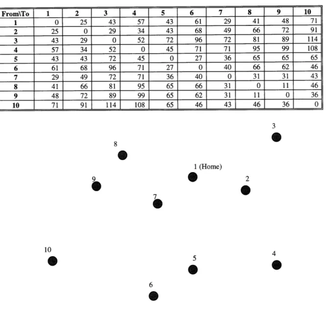
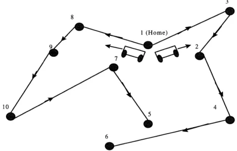
FIGURE 2-1: HOME AND NINE NODES TO BE VISITED ... ... 35
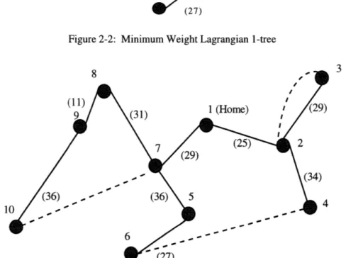
FIGURE 2-2: MINIMUM WEIGHT LAGRANGIAN 1-TREE ... 36
FIGURE 2-3: TEN-NODE PROBLEM AFTER THE MATCHING OF ODD-DEGREE NODES ... 36
FIGURE 2-4: THE FINAL SOLUTION TO THE MIXED ROUTING APPROACH... 37
FIGURE 2-5: Two ROUTES FOR TWO VEHICLES FOR THE MIXED ROUTING APPROACH ... 38
FIGURE 2-6: THE FINAL SOLUTION TO GREEDY ROUTING ALGORITHM ... 39
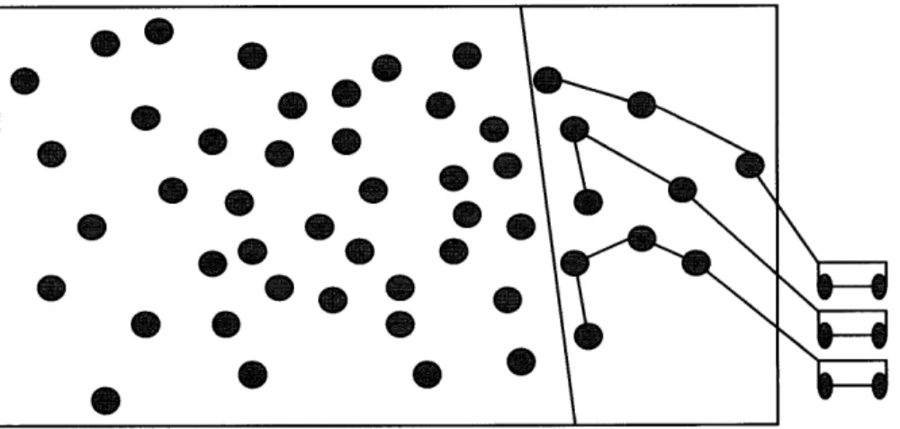
FIGURE 2-7: DIVIDED REGIONS USING SFCD ALGORITHM ... ... 40
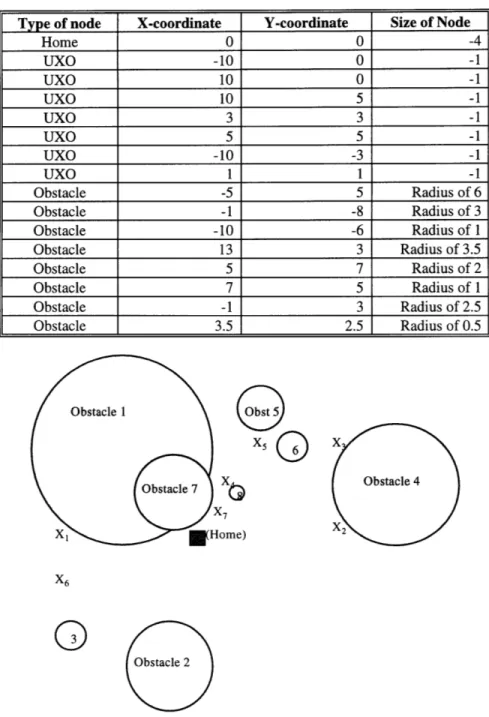
FIGURE 2-8: SEVEN UXO AND EIGHT OBSTACLES PROBLEM FOR WINNER ALGORITHM... 42
FIGURE 2-9: WINNER ALGORITHM'S FINAL PATH FOR ONE VEHICLE... 43
FIGURE 2-10: TWO MINIMUM SPANNING TREES FOR COMBINED ALGORITHM ... 44
FIGURE 2-11: ODD DEGREE NODES FOR COMBINED ALGORITHM... ... 45
FIGURE 2-12: THREE MINIMUM SPANNING TREES FOR COMBINED ALGORITHM ... 46
FIGURE 2-13: THE FINAL TOURS FOR COMBINED ALGORITHM... ... 46
FIGURE 2-14: FIRST AREA ROUTE PLAN FOR TOO MANY UXO PROBLEM ... 47
FIGURE 2-15: SECOND AREA ROUTES FOR TOO MANY UXO PROBLEM... 48
FIGURE 2-16: COMPOSITE PLAN FOR TOO MANY UXO PROBLEM ... 48
FIGURE 2-17: NINE NODES WITH THREE HOME NODES PROBLEM... 50
FIGURE 2-18: MULTIPLE HOME NODE ASSIGNED TO NODES FOR A = 1 ... ... 51
FIGURE 2-19: MULTIPLE HOME NODE ASSIGNED TO NODES FOR A = 0.5 ... 51
FIGURE 2-20: MULTIPLE HOME NODE ASSIGNED TO TWO VEHICLES WITH A = 1 ... 52
FIGURE 3-1: OBSTRUCTED VEHICLE FOR NINE NODES PROBLEM... ... 54
FIGURE 3-2: OBSTACLE AVOIDANCE FOR NINE NODES PROBLEM ... 54
FIGURE 3-3: OBSTACLE AVOIDANCE FAILURE FOR NINE NODES PROBLEM... 55
FIGURE 3-4: BY-PASS OBSTRUCTED NODE FAILURE FOR NINE NODES PROBLEM ... 56
FIGURE 3-5: SINGLE-GOAL RE-PLAN FOR NINE NODES PROBLEM ... 57
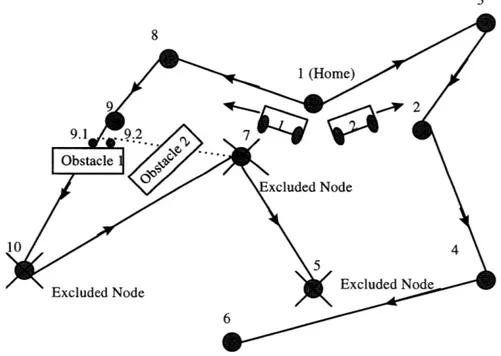
FIGURE 3-6: EXCLUDED NODES BY AN OBSTACLE ... ... 58
FIGURE 3-7: CANDIDATE CONNECTING PATHS TO CONNECT EXCLUDED NODES ... 59
FIGURE 3-8: THREE INITIALROUTES FOR THREE VEHICLES FOR DETONATED VEHICLE EXAMPLE... 60
FIGURE 3-9: EXAMPLE OF A DETONATED VEHICLE... .. ... 60
FIGURE 3-10: REASSIGNING ANODE FOR DETONATED VEHICLE ... 61
FIGURE 4-1: FIGURE 4-2: FIGURE 4-3: FIGURE 4-4: FIGURE 4-5: FIGURE 4-6: FIGURE 4-7: THREE MAIN FUNCTIONS OF THE MISSION MANAGER ... ... 63
A GRAPHICAL REPRESENTATION OF THE INPUT IN TABLE 4-1 ... 65
AN EXAMPLE OF INITIAL PLAN OUTPUT DATA FOR A SINGLE VEHICLE ... 66
GRAPHICAL REPRESENTATION OF ANINITIALPLAN FOR A SINGLE VEHICLE... 67
A SAMPLE OUTPUT FILE OF THE MISSION MANAGER ... 68
AN UNKNOWN OBSTACLE DETECTED DURING VERIFICATIONPROCESS ... 69
FIGURE 4-10: DETONATED VEHICLE DURING THE VERIFICATION PHASE... ... 72
FIGURE 4-11: RE-PLAN USING THE MULTIPLE-GOAL RE-PLANNER... ... 73
FIGURE 4-12: RE-PLAN USING THE SINGLE-GOAL RE-PLANNER ... ... 73
FIGURE 4-13: A SAMPLE SUMMARY OF ROAD-BUILDING MISSION... ... 74
FIGURE 5-1 INTERACTIONS BETWEEN MISSION COORDINATING SYSTEM AND SYSTEM SOFTWARE ... 77
FIGURE 5-2: INITIAL MISSION PLANNERFLOW DIAGRAM ... 79
FIGURE 5-3: VERIFICATIONMISSION MANAGER FLOW DIAGRAM... 80
FIGURE 6-1: GRAPHICAL REPRESENTATION OF THEKNOWN. OBST INPUT... 86
FIGURE 6-2: INITIALROAD-PLAN USING THE MIXED AND SFC COMBINED ALGORITHM... 88
FIGURE 6-3: GRAPHICAL REPRESENTATION OF THEKNOWN. OBST AND UNKNOWN. OBST INPUT ... 90
FIGURE 6-4: GRAPHICAL REPRESENTATION OF THE ACTUAL PATH USING THE MIXED AND SFC ALGORITHM ... 92
FIGURE 6-5: VEHICLE 2 BLOCKED BY AN UNKNOWN OBSTACLE... 93
FIGURE 6-6: A SUCCESSFUL OBSTACLE-AVOIDANCE MANEUVER... 94
FIGURE 6-7: AN OBSTACLE-AVOIDANCE MANEUVER FAILURE... ... 94
FIGURE 6-8: GRAPHICAL REPRESENTATION OF THE SINGLE-GOAL RE-PLAN FOR NODE 12 ... 96
FIGURE 6-9: GRAPHICAL REPRESENTATION OF THE SINGLE-GOAL RE-PLAN FOR NODE 11 ... 97
FIGURE 6-10: GRAPHICAL REPRESENTATION OF THE ACTUAL PATH USING FIRST RE-PLAN FOR NODE 12... 99
FIGURE 6-11: GRAPHICAL REPRESENTATION OF THE ACTUAL PATH USING FIRST RE-PLAN FOR NODE 11 ... 100
FIGURE 6-12: GRAPHICAL REPRESENTATION OF THE SECOND TIME RE-PLAN... 101
FIGURE 6-13: THE FINAL VERIFIED ROUTES FOR THE 20-NODE MISSION PROBLEM ... 103
FIGURE 6-14: MULTIPLE ITERATIONS ON ONE ROAD-BUILDING MISSION... 105
FIGURE 6-15: EFFECTIVENESS OFMULTIPLE VEHICLES WITH INCREASING NUMBER OF VEHICLES... 106
FIGURE 6-16: SIMULATED TEST RESULTS FOR THE TEN MISSION CASES... ... 107
FIGURE 6-17: EFFECTIVENESS OF THEPLANNER WITHNO OBSTACLES ... 108
FIGURE 6-18: PLANNING TIME FOR THE MISSIONS WITHNO OBSTACLES ... ... 109
FIGURE 6-19: EFFECTIVENESS OF THEPLANNER WITHNO UNKNOWN OBSTACLES ... 110
FIGURE 6-20: PLANNING TIME FOR THE MISSIONS WITHNO UNKNOWN OBSTACLES ... 110
FIGURE 6-21: MISSION PERFORMANCE WITH INCREASING UXO NODE ... 111
FIGURE 6-22: MISSION PERFORMANCE WITH INCREASING KNOWN OBSTACLES... 112
FIGURE 6-23: PLANNING TIME WITH INCREASING THE NUMBER KNOWN OBSTACLES... 113
FIGURE A-1: M ITY- 1 PROOF-OF-CONCEPT VEHICLE ... 127
FIGURE A-2: MITY-3 PROTOTYPE VEHICLE WITH CONICAL WHEELS AND AN INSTRUMENTAL ARM ... 128
FIGURE A-3: "COMPANION" PROTOTYPE VEHICLE - 5 FEET TALL ... ... 129
FIGURE A-4: DRAPER SMALL AUTONOMOUS AERIAL VEHICLE (DSAAV) ... 129
FIGURE A-5: VORTICITY CONTROL UNMANNED UNDERWATER VEHICLE (VCUUV) SYSTEM DESIGN... 130
FIGURE C- 1: TRAVEL GRID WITH TIMES TO TRAVEL EACH LEG... 138
FIGURE C-2: TRAVEL GRID WITH TIMES TO TRAVEL AND THE OPTIMAL COST-TO-GO ... 139
FIGURE C-3: DEPOT AND NINE NODES TO BE VISITED... 141
FIGURE C-4: MINIMUM SPANNING TREE FOR LAGRANGIAN ... 141
FIGURE C-5: MINIMUM WEIGHT LAGRANGIAN 1-TREE... 142
FIGURE D-1: MINIMUM SPANNING TREE PROBLEM ... 143
FIGURE D-2: NINE STAGES OF THE MINIMUM SPANNING TREE BY USING GREEDY ALGORITHM... 144
FIGURE D-3: CONCEPT OF THE CLARKE-WRIGHT SAVINGS HEURISTIC... 145
FIGURE D-4: FINAL TOUR FOR CLARKE-WRIGHT SAVINGS ALGORITHM ... 147
FIGURE D-5: THE OPTIMUM TOUR USING CLARKE-WRIGHT SAVINGS ALGORITHM... 148
FIGURE D-6: EXAMPLE INSERTION PATTERNS FOR THE PAIR INSERTION HEURISTIC ... 149
FIGURE E-1: Two PATHS FOR THE Two VEHICLES USING DYNAMIC PROGRAMMING... 153
FIGURE E-2: DIVIDED REGIONS FOR THREE VEHICLES USING DYNAMIC PROGRAMMING ... 154
FIGURE E-3: THREE INDIVIDUALROUTES FOR THREE VEHICLES USING DYNAMIC PROGRAMMING... 155
FIGURE E-4: SIMULTANEOUS ASSIGNMENT OF NODES USING DYNAMIC PROGRAMMING... 155
FIGURE E-5: EXAMPLE OF How Two NODES CAN BE VISITED AT THE COST OF ONE ... 156
FIGURE E-6: Two ROUTES FOR Two VEHICLES USING PAIR INSERTION ... . 157
TABLE 2-1: COMPARISON OF HEURISTIC AND EXACT PROCEDURES ... 30
TABLE 2-2: DISTANCE MATRIX FOR HOME AND NINE NODES ... ... 35
TABLE 2-3: ANGLE INFORMATION FOR NINE NODES FOR SFCD ALGORITHM ... 41
TABLE 2-4: COORDINATE MATRIX FOR THE WINNER ALGORITHM EXAMPLE ... 42
TABLE 2-5: GROUP OF NODES FOR WINNER ALGORITHM... ... 43
TABLE 2-6: QUANTITY R(I) FOR MULTIPLE HOME NODE PROBLEM ... ... 50
TABLE 4-1: AN INPUT DATA FILE TO THE INITIAL MISSION PLANNER... ... 64
TABLE 4-2: DISTANCE MATRIX OF THE EXAMPLE INPUT INFORMATION ... 66
TABLE 4-3: CONNECTIVITY MATRIX OF THE EXAMPLE INPUT INFORMATION ... 66
TABLE 4-4: A SAMPLE INPUT FILE FOR THE UXO-CLEARING PLANNER... 75
TABLE 5-1: NODE TYPE DEFINITION IN ANINPUT DATA FILE ... ... 78
TABLE 6-1: SIMULATIONPARAMETERS FOR CONSISTENCY TEST ... 105
TABLE 6-2: SIMULATION PARAMETERS FOR THE MISSION WITH THEVARYING NUMBER OF VEHICLES... 106
TABLE 6-3: SIMULATION PARAMETER FOR THE NO OBSTACLE CONDITION TESTS ... 108
TABLE 6-4: SIMULATION PARAMETER FOR THE NO UNKNOWN OBSTACLE CONDITION TESTS ... 109
TABLE 6-5: SIMULATION PARAMETER FOR THE MISSION CASES WITH VARYING NUMBER OF UXO NODES ... 111
TABLE 6-6: SIMULATION PARAMETER FOR THE MISSION CASES WITH VARYING NUMBER OF KNOWN OBSTACLES ... 112
TABLE C-1: COMPLEXITY OF THE BRUTE FORCE METHOD AND THE DYNAMIC PROGRAMMING METHOD. 142 TABLE C-2: DISTANCE MATRIX FOR DEPOT AND NINE NODES ... 142
TABLE D-1: CLARKE-WRIGHT SAVINGS LISTED IN DECREASING ORDER ... 149
Chapter One : Introduction
The application of robotics solutions to the problem of collecting and disposing of unexploded munitions offers the obvious benefit of reducing the risks to human life which the task would otherwise involve. To the extent that the robots can carry out their tasks autonomously, human workload is reduced, which is another benefit. If the target munitions are dispersed over a fairly wide area, then the use of multiple robots will reduce the time required to collect them. In this thesis and in Bryan Koontz's thesis [10], an approach to the problem based upon a centrally-controlled multi-vehicle autonomous robotic system is described. An introduction to the EOD (Explosive Ordnance Disposal) mission as currently performed is given below.
1.1 EOD (Explosive Ordnance Disposal) Mission
According to the Boston Globe, 110 million land mines reside in the world. The United States estimates that it will take more than 1,000 years to remove these mines at the current rate of clearance and will cost $33 billion to remove the mines that are already deployed. Furthermore, 2 to 5 million new land mines are deployed every year while only 100,000 mines are cleared [5]. Also, unexploded ordnance (UXO) reside in millions of acres of property in the United States due to the weapons system testing and troop training activities [14]. Furthermore, only 3,000 EOD technicians are available in the United States, and they must complete other tasks than clearing UXO [9].
Clearing UXO is currently a slow and dangerous process that exposes military personnel and expensive equipment to significant risk. The current manual UXO clearing process involves partitioning potential areas of having UXO into sectors with corners indicated by bright colored flags. A four-to-eight-man team is sent to visually sweep the area for UXO in each sector. Figure 1-1 depicts the terrain and natural obstacles that would present a challenge to robotic vehicles. All military personnel except the Marines carry out blow-in-place (BIP)' process when a UXO is detected. The Marines carry out the manual pickup and carry-away (PUCA) process to collect the UXO in an ordnance disposal area (ODA) to detonate later [9]. Figure 1-2 displays the variation in size, shape, and appearance of the UXO collected in a PUCA mission.
Figure 1-1: Sweep Team Looking for UXO
Figure 1-2: UXO Gathered by the Sweep Team in a PUCA Mission
The risk is considered much greater in clearing the UXO than manually sweeping for the UXO. Three categories of UXO excavation technology are available for the military personnel. The oldest UXO excavation technology is the manual methods, which basically use shovels and other digging tools to excavate soil around the potential UXO. These methods present the most risk to the personnel. More upgraded methods use mechanized systems such as bulldozers, front-end loaders, and other heavy construction equipment. These methods produce faster and more efficient excavation than the manual methods. The most advanced excavation technology uses remote-controlled systems such as telerobotic and autonomous systems. These last methods provide the highest degree of safety to the personnel [14].
The UXO clearing process is not only labor intensive and dangerous, but also expensive. For example, DoD estimates to clear a 28,800 acres of property in Kaho'olawe Island, Hawaii is approximately $400 million, or about $14,000 per acre [14]. Therefore, the Research and Development Department of the Naval Explosive Ordnance Disposal Technology Division (NAVEODTECHDIV) is currently conducting a research and development program for small autonomous robots system to carry out PUCA and BIP processes.
The main objective of this thesis is derived directly from the functional requirements of the overall EOD mission, which is to clear UXO in an efficient manner. The main objective of the EOD mission is to provide affordable but autonomous robotics technology to clear UXO safely while reducing the number of personnel required. A multiple robotic vehicles system is an ideal selection to fulfill the overall EOD requirements. However, multiplicity and autonomous aspects require more advanced and efficient strategies for UXO retrieval. An autonomous mission manager provides a complex but efficient solution for UXO retrieval by a multiple vehicles system. Dividing the problem into two subsystems, namely planning and mapping, reduces the complexity of the mission manager system [9]. Furthermore, the management system is even more simplified by dividing into two distinct phases, which are the road-building, and clearing phases. These phases not only relieve the complexity of the mission manager but also present a more efficient way to carry out UXO retrieval processes.
1.2 Objectives
The objective of this thesis is to provide an efficient and effective mission manager to assign and control multiple vehicles to obtain obstacle-free roads, which assigns UXO nodes to multiple vehicles and creates obstacle-free roads along which they are visited. The manager must dynamically re-plan the vehicle paths as initially unknown obstacles are encountered. The objective is not to find the optimum paths, but to
1.3 Overview
Chapter 2 describes the initial mission planner in detail and addresses some additional challenges and issues. This chapter also includes some optimization background information related to the vehicle routing problem, including approaches for optimal, sub-optimal, and mixed solutions to the problem. Chapter 3 describes plan verification and planning, discusses challenges and issues, and describes a planner that re-plans for certain situations. Chapter 4 describes the mission manager and includes an extensive procedural steps along with the detailed explanations of the initial planner and verification manager procedures. Chapter 5 describes the implementation of the mission manager including the planning and managing architecture. The chapter briefly explains the simulation of the various tests to evaluate the mission manager. Chapter 6 includes several tests that have been run on the two implemented road planning algorithms to make comparisons between the algorithms. This chapter also describes the tests on different cases to evaluate the effectiveness of the management and coordination mechanisms, particularly for the road-building phase, and discusses the results of those tests. Chapter 7 concludes the thesis with a summary of the project, the merits of approaches to the road-building phase, and suggested areas for further research and development.
1.4 EOD System
The mission manager is part of an overall SMART system. To better understand the constraints of the problem and the information available, the solution sections describe the elements of the SMART system. These elements include the hardware, software, and the global positioning system. The configuration of the EOD robotic vehicles has evolved from current proven designs through both hardware and software testing. The baseline of the vehicle, the MITy-2, is a 6-wheel drive flexible frame micro-rover driven by battery power (Figure 1-3). Two new developments, which are the UXO local detection sensor and UXO
manipulator system, are required for the EOD vehicles. These new developments are minimal compared to alternative totally new mobility concepts. The EOD project is one of the important robotic projects in IUVC (Intelligent Unmanned Vehicle Center). Refer to the Appendix A for the history of IUVC and descriptions of other on-going or past robotic projects.
Inclinometers Sun Sensor Gyro Laser Range Finder
Bumper Drag Wheel
Proximity (not shown)
Sensors
Figure 1-3: MITy-2 Micro-Rover
1.4.1 Hardware System
Both the hardware and software architectures of the EOD vehicle have been derived from the MITy-2. Two EOD vehicle prototypes (Figure 1-4) have been designed and built to test the feasibility of the EOD vehicles system for Mine Countermeasure operations. The baseline EOD vehicle is a 6-wheel drive flexible
frame, which provides a high degree of maneuverability, driven by power generated by a small 12V DC
motor. This six-wheel drive generates speed of the vehicle up to 6 fps or 1.8 mps [11].
Figure 1-4: EOD SMART Vehicles
BUMPER GRAPPLER I Motor GRAPPLER 2 MOTOR Motor SONAR METAL DETECT LFRONT PLurrTru
POWER DRI VER.S... ... .
BATTERYR REGD MOTOR :REAR PLATFOR ... M OTOR
MOTOR
.... M......
The flexible frame includes three individual platforms connected by flexible wires. Additionally, they are equipped with front and rear Ackerman steering mechanisms2 and a modular chassis. The front
platform includes a metal detecting unit, sonar electronics, a bumper, and the 2-DOF manipulator to acquire
UXO with a metal detecting unit embedded in the base of the acrylic manipulator bed. The middle platform
contains an onboard microprocessor, gyro, video camera and transmitter, serial modem, LPS (laser positioning system) transponder, and control circuitry. Lastly, the rear platform includes power regulation circuitry and battery packs (Figure 1-5) [11].
1.4.2 Software System
The software architecture for the EOD system is divided into two main areas: 1) onboard control software, and 2) control and ground station software. All software is developed under Linux. Onboard control software is programmed using C, then the software is compiled using a program "Dynamics C" to be downloaded to the processor on the vehicle. The ground station software is coded using C and the GUI (graphic-user-interface) is programmed using Motif. The ground station is located in a Pentium computer. The onboard control software is initially located in the same computer; then the control software is transferred to the processor on the vehicle.
1.4.2.1 Onboard Control
The onboard software for each of the vehicles is based on hierarchical design. This software is divided into layers, in such a way that the code for a layer depends only on the layers below itself. Thus, a lower layer would not be able to control a higher layer than itself. Any changes to a particular layer will thus only influence higher layers. The onboard control software includes code for handling high-level tasks, which let the vehicle complete a simple goal such as navigating to a point, initiating an area search for UXO, or picking up a detected UXO [11]. The control software can easily be expanded by adding layers or tasks. Most of the high-level task processing is done on the control or ground station since the onboard processor has limited memory.
1.4.2.2 Ground Station
The ground station will communicate with each of the vehicles to receive telemetry and task-related data and to send task commands. The ground station carries out high-level mission control and
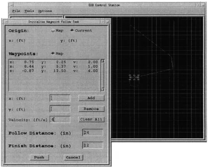
management tasks. Figure 1-6 displays the control or operating station GUI. The mission control window interfaces the vehicle to the ground station (Figure 1-7). Some of the elements on this control window are the current assigned task, the current position, heading, and velocity of the vehicle. Multiple overlays displaying obstacles, sonar pings, path history, planned tasks, and a map grid can provide an overhead view of the vehicle but can be hidden if desired. Task parameters appear on the ground station display when a task needs to be created. Teleoperation or supervisory control of the vehicle is also supported to allow human operator interaction if needed [ 11].
The ground station for the EOD mission has two coupled tasks for path planning. The first task involves mapping with environmental information, to provide an updated map of the mission field at every cycle. This map contains the locations of UXO, known obstacles, and detected obstacles during the exploration phase. This structure combines global and local maps into one map to prevent confusion about the obstacle locations during the operation. This concept allows the dynamic growth of the map by providing speed and memory increases [18]. These capabilities will allow UXO clearance mission to be as autonomous as possible.
The second task (i.e. search) finds a path that minimizes a cost function between a start node and a final or goal node using the updated map. An A* algorithm that tries to find a path with the minimum cost has been developed [16]. Unlike Dijkstra's algorithm [15], which is a brute force method, the A* algorithm uses heuristics to yield a shortest path between two nodes in a reasonable time but not the optimal path.
2 This steering method is based on a design that terminates the center point of each wheel at a common point. The use of this type of
This algorithm doesn't do an exhaustive search to minimize searching time [10]. Therefore, trades must be made between obtaining the optimal solution and generating the solution in the minimum time [3].
Figure 1-6: Control Station GUI Showing the Map Overlays and Available Mission Tasks
Figure 1-7: Control Station GUI Implementing a Waypoint-Follow Task
1.4.3 Global Positioning System
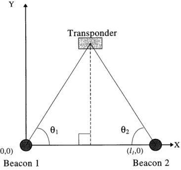
A laser positioning system (LPS) is used to correct navigational error from the dead reckoning system. This absolute positioning system provides a verification of vehicle's position using two synchronized laser beacons and onboard transponders (Figure 1-8). If the distance, 1 , between the two beacons is known then
the angles 0 1 and 0 2 (calculated based on the timing sequence given by the transponder on the vehicle)
can be used to compute the vehicle position [11].
Y
Trans onder
01 02
(0,0) (l,0)
Beacon 1
Beacon 2
Figure 1-8: Laser Positioning System (LPS)
1.5 Requirements for the Autonomous Mission Manager
The locations of the UXO are known within the area of operation a priori3; however, the environmental
conditions are not known a priori. The initial assumptions for the locations of the UXO are provided by a manual visual sweep, air or satellite reconnaissance, or an automated UXO survey vehicle [9]. In addition, the robotic vehicles should be able to do search task for the UXO within a given 1 m2 area. Despite the small area to be searched, the vehicles must be able to pinpoint the exact location of the UXO. Since the terrain conditions are not assumed to be known initially, the robotic vehicles must also be able to avoid obstacles. A remotely located operator will monitor the multiple vehicles as well as coordinate activities for the PUCA operation. The operator station should be located at a safe distance from the area which contains potential UXO and the ODA. The use of the operator station will allow a single worker to safely
accomplish the work that now requires and risks many ordnance disposal technicians.
In order to carry out the basic mission, multiple robotic vehicles must be coordinated and controlled. The vehicles are able to carry out simple tasks autonomously such as waypoint follow, obstacle or hazard avoidance, search, pick-up, drop-off, and others. The vehicles and the ground station will communicate by a two-way wireless link. However, the vehicle is not able to communicate to other vehicles in the field. Therefore, an operator or control station needs to coordinate the multiple vehicles. This operator station contains environmental information and vehicle information so that it can plan a series of commands and determine optimal routes for each of the vehicles. The hazard and location telemetry information from each of the vehicles is used to update the map on the operator station to do re-planning if required. Therefore, the key elements of an efficient autonomous vehicle(s) system are information fusion and vehicle management. The coordination of the vehicles can be accomplished more efficiently by an automated mission management system (Figure 1-9) on the ground station [9].
Using the planning and mapping capabilities, the mission manager can accomplish the UXO clearance mission by means of two distinct phases. The first phase is the "road-building" which tries to find
free roads using the full capability of the sensors on the vehicles. Then, the "UXO-clearing" phase uses the network of obstacle-free roads to plan to actually clear the given field.
Figure 1-9: Automated Mission Management System
1.5.1 Road-building Phase
At the beginning of the UXO clearing mission, the EOD vehicle are assembled at an ODA located at one corner of an area that contains the potential UXO (Figure 1-10-I). The planning subsystem uses given locations of potential UXO to assign a sector to each of the available vehicles. Then, the manager generates a plan that assigns some UXO to each of the vehicles to visit using the slow speed mode4. This mode allows navigation through an unknown environment with obstacle avoidance. When the vehicle reaches the final UXO in its assignment, it picks up that UXO and returns to the ODA in a fast mode retracing its returning path. It then repeats this process for the second-to-last UXO (and so on) using the fast mode
along the verified road. However, in the face of uncertainties such as detecting an obstacle in the assigned path or a detonated vehicle, several intermediate steps will occur during this road-building phase.
Therefore, the mission management must be designed to deal effectively with the unexpected events such as detecting an unknown obstacle in the assigned road (Figure 1-10-HI). If an obstacle interferes with a vehicle's plan so that one or more UXO do not get covered, then the mission manager needs to either re-assign the excluded UXO or re-plan at the moment of discovering an unexpected event during the mission (Figure 1-10-IV) [9]. The mapping subsystem stores the locations of detected obstacles in the UXO area as well as the established obstacle-free roads. The entire research of this thesis is devoted to create an automated solution to approach the road-building phase of the EOD mission. Thus, the remaining chapters will concentrate on the road-building aspect of the EOD mission.
I II
III IV
LEGEND
0 uxo Obtacle
SBU.G .... Road cergment
-- P lamed rout UIXO em oved
egm ment -.- BUG path
Figure 1-10: Illustration of the Road-Building Approach to UXO Clearance (I) Basic UXO Gatherers (BUGs) and Assigned Routes to UXO (II) The Slow Outward Path of One BUG and Its Fast Return with the Furthest UXO (III) One BUG Can Not Visit an Assigned UXO Location Due to Unforeseen Obstacles (IV) A New Plan Incorporating More Information
1.5.2 UXO-Clearing Phase
The mission manager uses the established obstacle-free roads to assign vehicles to proceed to each
UXO at a much faster pace. The planner creates plans that optimize the tasks of clearing UXO on the
established roads.
Bryan Koontz, another MIT graduate student, has developed an autonomous mission manager or planner for multiple vehicles system to clear UXO from a network of obstacle-free roadways. The approach to plan the UXO clearance borrows ideas from the fields of Game Theory, Graph Theory, Topology, and concepts in basic robot motion planning. In his thesis, the area to clear is treated as a simply connected and undirected network with the locations of the potential UXO as nodes [9]. The concept of competition among the individual vehicle is used throughout the algorithms. In other words, an individual vehicle competes for free space on the network with other vehicles to find an optimal path for its assigned route. On the other hand, the mission manager works to find an optimal path for each of the vehicles to reach a goal configuration on the network, which is the "road-map" such that no interference occurs between the vehicles [9]. Refer to the thesis "A Multiple Vehicle Mission Planner to Clear Unexploded Ordnance from a Network of Roadways" for more details on the UXO-clearing subject of the EOD mission.
1.6 Road-Building Manager
The road-building problem has two aspects. The first aspect, initial planning, involves creation of the initial pathways. The second aspect, verification, enables the system to re-plan or to adjust the current plan to meet new conditions. The initial planning and plan verifying solutions are coupled to form a closed-loop process in the multiple vehicle manager system (Figure 1-11). This closed-loop process allows the system to re-plan if conditions at the time of plan verification diverge from the conditions considered at the time of plan creation [6].
Road-Building Management
Road Planner Road Exploration
Road Re-Planner g Road Verification
Figure 1-11: The Coupled Closed-Loop Process of the Road-Building Management System The objective of optimizing the planning problem is to provide feasible plans and to meet the goals in such a way that the maximum planning optimization is acquired while minimum resources such as time, fuel, or money are utilized. In the road-planning case, the objective is to find a path that connects all the dispersed UXO with the minimum distance traveled by each of the vehicles or the minimum total time spent to find the path. The road-building phase initiates with an initial plan or a series of commands and follows the commands until conditions change in the environment. The initial plan is followed closely when possible and provides a basis for creating a new plan if the current plan is no longer feasible [6].
1.6.1 Initial Mission Planner
In the road-building phase of the EOD mission, the locations of UXO or nodes are predefined. Using some well-structured planning algorithms, a plan that connects the given nodes without violating any constraints is created. Although an initially planned route will likely be modified several times during the execution phase, an initial plan will definitely save time and difficulty in covering specific nodes. To enable the planning process, the nodes in the problem are classified as visited UXO, unvisited UXO, disposal location, home (service station), or obstacles. Refer to the Chapter 2 for more detailed descriptions of the planning algorithms to create an initial plan for the EOD road-building mission.
The initial mission planner creates road plans around any predefined obstacles for the vehicles to cover the least distance during the verification phase. This initial road plan should be identical to the verified road plan so long as the environment and constraints don't change during the verification phase. However, the initial plan will almost always change during the verification phase. Thus, some method of managing the problems that come up during the verification phase must be provided.
1.6.2 Verification Mission Manager
During initial planning, the verification of an initial road plan has not begun yet. Verification is actually accomplished by sending the vehicles along the initially planned roads to visit the nodes on the roads. During the verification phase, the vehicles must travel at low speed to allow time for the sensors to detect and avoid obstacles. At the verification stage, the vehicles visit the nodes and verify that the roads are free of obstacles. If the vehicles discover that the roads are not free of obstacles during the verification phase, the manager needs to re-plan. If the manager determines that a vehicle is lost (i.e. detonated), then the manager has an option to request a re-plan using the updated environmental information. Likewise, if a
vehicle reports that it has completed its assigned task earlier than the other vehicles, then the manager has an option to request a re-plan.
Separate representation and storage for the planned and verified roads are required during the verification phase. Planned roads are assumed initially to be obstacle-free and the verified roads are
actually obstacle-free roads. Thus, if any successful obstacle-avoidance maneuver takes place, then the segments that are added by the maneuver must be stored among the verified roads. On the other hand, if any unsuccessful obstacle-avoidance maneuver takes place then the segments that are blocked by the obstacle must be eliminated. The excluded node must be stored separately to plan to visit later in the road-building phase. Therefore, the verified obstacle-free roads must be stored in a separate storage for later use particularly to carry out UXO-clearing process.
The main objective of the verification mission manger is to execute, verify, and modify (correct) an initial plan that is passed from the initial planner. If an obstacle or problem arises during the verification process that will keep vehicles from further traveling, then the mission manager must provide re-plans. The mission manager usually tries to generate the modified plan that will most likely optimize the use of the remaining resources. However, modified plans may not be the optimal solution since this plan modifying process only optimizes immediate parts of the problem. Refer to the Chapter 3 for more detailed
Chapter Two : Initial Planning
Given a list of the locations of UXO, an initial mission planner can generate an initial plan for any number of vehicles that connects all the given nodes in an area. The initial planner provides a connected path for each of the available vehicles. The number of UXO that must be visited are divided among the multiple vehicles to reduce the workload and time to cover a specified region. The main objective of the initial mission planner for road-building phase is to create a feasible plan in the shortest time possible. An initial plan is likely to change during the verification process due to the uncertainty in the terrain (i.e. obstacles). Thus, spending a long time on an initial road plan is inefficient and unnecessary.
2.1 Problem Definition
An optimal initial plan for the road-building phase is a route that connects all the given UXO nodes with the minimum time or distance. This problem basically becomes a node-covering one such as the traveling salesman problem (TSP) or vehicle routing problem (VRP) 5 if no obstacles are present. TSP and VRP are the most studied problems in the operations research and applied mathematics literature. Both the TSP and VRP are NP-complete problems. The TSP requires (n-1)! different orderings of the points to be visited where, n is the number of nodes to be visited. In other words, there are (n-1)!/2 different solutions since each tour can be run in either of two directions. Thus, a TSP with 10 nodes yields 1,814,400 possible solutions.
The EOD vehicle routing problem is equivalent to a VRP rather than a TSP. The basic VRP problem involves the routing of a vehicle or vehicles from a central depot to a set of dispersed demand points to minimize the total travel costs or time spent. Similarly, the EOD vehicle routing problem involves the routing of a vehicle or vehicles from any location to pre-defined locations of UXO to minimize the total travel distance or time spent [2].
2.2 Options for the Road Planning Algorithm
An initial plan may be derived from a model of the local delivery or pick-up vehicle routing and scheduling problem. The VRP has both optimal or exact solutions and sub-optimal or estimated solutions. Finding exact solutions to a small (less than 50 nodes) VRP is a difficult and inefficient task. All of the known exact solution algorithms grow exponentially in computation time as nodes are added. Storage requirements can be reduced by constraint windows such as limitations on the vehicles, time windows, and/or quality-of-service constraints. However, the required storage still grows an exponentially for exact solutions. For instance, an exact algorithm based on the idea of dynamic programming is O(n22n) where n
is the number of nodes. This type of algorithm also requires computer memory storage equivalent to n2n.
Therefore, exact algorithms become impractical as the number of nodes gets larger (around 70 nodes) [12]. There may never be an efficient algorithm for exact optimal solution to the TSP and VRP.
On the other hand, heuristic algorithms lead to reasonable or good but not necessarily optimal solutions at reasonable computational costs. The computation time for sub-optimal or heuristic solution algorithms grow as low order polynomials. These heuristic algorithms have been experimentally proven to work well
[4]. A mixed routing algorithm that is a combination of exact and heuristic methods also exists for the TSP and VRP [12].
Table 2-1 compares heuristic and exact procedures. Heuristic methods are compared to the exact algorithms, specifically dynamic programming and branch-and-bound methods. This Table illustrates that the exact algorithms are far less efficient than a general heuristic algorithm [7].
Table 2-1: Comparison of Heuristic and Exact Procedures Number of 6 7 8 9 10 16 Nodes Number of 2 2 2 2 3 2 Vehicles Constraint 13 3 9 5 7 7 General 26.0 119.0 16.8 56.0 17.2 19.8 Heuristic Solution Total Time7 0.048 0.066 0.063 0.075 0.107 0.189 Branch-and- 26.0 114.0 16.8 54.0 17.2 19.2 bound Solution Time8 0.5 0.2 0.8 245.0 1.31 80.1 Total Time7 74.5 NS/7009 NS/30009 NS/7009 2000 NS9 Dynamic 26.0 114.0 16.8 53.0 17.2 NS9 Programming Solution Total Time7 74.5 NS/7009 NS/30009 NS/7009 2000 NS9 2.2.1 Optimal Solutions
The largest vehicle routing problem of any complexity that has been solved exactly and completely is only 23 nodes. Four general algorithms exist for the exact TSP solutions. These algorithms are branch-and-bound, integer programming or ordinary linear programming, dynamic programming, and Lagrangian relaxation. All of the four algorithms for the exact TSP solutions can be modified slightly to solve the VRP as well. Both branch-and-bound and integer programming are types of general algorithms for integer linear programming (ILP). ILP is often referred to as the enumerative algorithm and is based on intelligent enumeration of all possible solutions. The enumerative algorithms use sub-tour10 elimination methods. Thus, branch-and-bound and integer programming overlap to some extent [16]. Refer to the Appendix C for the details of the optimal solution algorithms.
2.2.1.1 Branch-and-Bound
The first technique is a branch-and-bound (Appendix C, C. 1). The branch in a branch-and-bound refers to successive partitioning of the solution space. The bound refers to lower bounds that are used to construct a proof of optimality without exhaustive search. A branch-and-bound method is probably the most common type used for the TSP [15].
2.2.1.2 Integer Programming
The second technique is an integer programming or ordinary linear programming (Appendix C, C.2). This category of ILP is often referred to as the cutting-plane algorithm. The cutting-plane "cuts away" the non-integer parts of the feasible convex hull of the relaxed linear program by using hyper-planes. The hyper-planes represent constraints that have been generated in the linear programming calculations. These constraints are considered in such a way that no feasible integer solutions are ignored [1].
6 The 6, 8, 10, and 16 node problems used a travel time constraint on each vehicle. The 7 and 9 node problems used a maximum number of nodes per vehicle constraint.
7 Total CDC6500 CPU time (in seconds) to complete the calculations. 8 CDC6500 CPU time (in seconds) to find the best solution.
9 NS = Not solved. NS/700 = Not solved in 700 seconds of CDC6500 CPU time.
10 A tour is a path around a network that includes each node once and starts and stops on the same node. A sub-tour is a tour that does not pass through all nodes of the network.
2.2.1.3 Dynamic Programming
The third technique is dynamic programming (Appendix C, C.3), which has been used less on the TSP. The main drawback of this method is the computer storage requirements. The combinations grow
exponentially with the complexity of the problem. For instance, the core storage requirements to solve a 20 cities TSP exceeds 900,000 words. However, this algorithm is the only exact solution that appeared promising for finding the optimal solution of VRP [1]. Thus, dynamic programming can be extended to solve MVRP (Appendix E, E. 1). Dynamic programming is similar to a branch-and-bound method in the sense that it considers all the feasible solutions. However, this method works backward from the last decisions made. The idea is to break down the problem into steps, make decisions at each step, and find a recurrence relation between a step and the previous step.
2.2.1.4 Lagrangian Relaxation.
As the problem size increases the lower bounds in a branch-and-bound algorithm increases due to the several repetitions of the sub-tours. The main constraints in the TSP are the requirements of the vehicle to visit each node exactly once. These constraining equations usually create complications in computing a tight lower bound. Rather than totally ignoring the constraints for simplicity, an alternative way such as a Lagrangian techniques (Appendix C, C.4) can be applied to relax the constraining equations. This technique is basically mathematical manipulations that penalize constraint violations and reward constraint satisfactions. In other words, a penalty term from the constraint violations or the reward term from the constraint satisfactions is added to the cost function [16].
2.2.2 Sub-Optimal Solutions
A general TSP that can be solved optimally or exactly is limited to about 100 nodes or less. The limit
on time and computer storage drives the limitation of the nodes in a problem. Furthermore, this limitation is much more severe for the VRP due to the complexity in the computations. VRP is a subset of TSP (i.e. VRP is a constrained TSP). VRP is much more complex due to the vehicle constraints or limits on capacity and operation. The added constraints make the computations much more difficult. However, the same constraints eliminate some of the searches in the problem. Still, problems with a large number of nodes are impractical to solve optimally. However, many heuristic approaches that yield sub-optimal solutions are available to solve large problems [1].
Heuristic procedures are generally categorized into three broad classes: tour construction heuristics, tour improvement heuristics, and composite heuristics. Tour construction approaches always begin the process with a single node and add nodes to build a complete tour. Tour improvement approaches start with the initial tour obtained in the tour construction procedure and try to improve the tour. Lastly, composite approaches are a combination of the first two approaches. These procedures construct an initial tour by using the tour construction approaches and improve the initial tour by using the tour improvement approaches [4]. Refer to the Appendix D for the details of the sub-optimal solution algorithms.
2.2.2.1 Tour Construction Heuristics
Tour construction procedures create a complete tour that visits one node at a time by using the known distance or cost matrix. This procedure adds a node to the partially constructed tour in the VRP only if it will be included in the final solution. Experimental results show that tour construction heuristics generally don't produce good results. Nevertheless, many tour construction procedures are available to construct an initial tour for any given problem with or without constraints. Some of the heuristic methods are the nearest neighbor or greedy algorithm, the Clarke-Wright savings algorithm that usually solves the VRP, and pair insertion procedures [1].
Nearest Neighbor/Greedy Heuristics
A nearest neighbor or a greedy method (Appendix D, D 1.1) is the simplest of all heuristic methods available. This method suggests beginning at the depot and always selects the nearest unvisited but feasible
node to be the next visit until a complete tour is achieved. The advantage of the method is its simplicity of representation and implementation. A greedy heuristic is much simpler to implement than either a Clarke-Wright savings or a route insertion algorithm. However, this simple method usually doesn't create good tours for either the TSP or the VRP [1].
Clarke-Wright Savings Heuristics
Dantzig and Ramser were credited with developing the savings heuristics to solve the VRP specifically. Clarke and Wright also developed a savings heuristic (Appendix D, D. 1.2), but with numerous
modifications, to solve the VRP. As stated above, this procedure starts by choosing any node (usually the depot) as the origin of the tour. The procedure also assumes initially that every node in the problem is visited from the selected origin. Then the savings from combining two sub-tours into one node are
calculated for all the nodes. The complete tour is constructed in the order of the decreasing savings that are computed without violating any constraint.
Pair Insertion Heuristics
An insertion procedure (Appendix D, D. 1.3) basically produces a feasible tour by adding one node at a time to a sub-tour. This procedure applies a specific selection rule that selects an unvisited arbitrary node and suggests where to insert this node in the partial tour. The types of selection of the next node to be included in the final sub-optimal tour are the nearest, farthest, and random relative to any one of the nodes in the partial tour. The sub-optimal solutions discovered by the insertion procedure are within 3-5% of the optimal solution for a single VRP [1].
2.2.2.2 Tour Improvement heuristics
Tour improvement heuristics begin with a provided feasible tour to yield a better and improved tour. Two of the tour improvement heuristics have been applied to the TSP and VRP. The first method is the r-optimal heuristics (Appendix D, D2) that produce tours at least as good as those resulting from the Clarke-Wright savings method. The other method is the X-optimal heuristics created by Lin and Kernighan. They both use the arc interchange or branch exchange technique to improve the current tour [1].
2.2.2.3 Composite Heuristics
The composite heuristics (Appendix D, D.3) are a combination of the tour construction and improvement heuristics. This procedure generates an initial tour by the tour construction method and improves the tour by the tour improvement method. The composite technique should always produce results at least as good as the tour from tour construction method without the improvement method [1].
2.2.3 Mixed Solutions
The mixed solution method is a combination of the optimal and sub-optimal algorithms (Appendix D, D.4). Mixed routing algorithms exist in many different forms. A particular mixed routing approach that was considered for EOD VRP is a combination of Lagrangian 1-tree and tour improvement heuristics. This algorithm is a combination of the exact and estimated solution method. The particular mixed routing algorithm that has been considered for EOD VRP involves three major steps. The fourth step is optional and may improve the solution further. The algorithm also results in a tour that is guaranteed to be less than 50% longer than the optimal tour. Section 2.3.1 explains the algorithm in detail and provides an example to demonstrate the steps in the algorithm.
2.2.4 Extended Solutions
The various algorithms that are explained previously solve a single VRP or single TSP. However, the EOD vehicle routing problem deals with multiple vehicles. Therefore, the algorithms that solve single VRP or TSP need to be extended to the multiple vehicles case. The multiple vehicles routing problem (MVRP)
is harder to solve than the single vehicle routing problem whether an exact or heuristic algorithm is used. Most of the exact algorithms are ineffective to solve the MVRP primarily due to the complexity of the problem. Some of the heuristic algorithms are not efficient to solve the MVRP as well.
Any of the algorithms for the single VRP or TSP can be used for two vehicles without much modification. In fact, the same exact tour found using the previous algorithms can be applied to the two vehicles routing problem. The only difference is that the nodes in the tour are divided and assigned to two vehicles instead of just a single vehicle. The tour can be easily divided into two different paths: one in each direction from the depot or origin node. The two paths would be approximately equal in distance so that the two vehicles can cover roughly equal distance. However, the number of nodes may not be equally distributed along the two paths. Therefore, one vehicle may visit more nodes than the other vehicle. Thus, the two paths along the tour allow the two vehicles to build the routes simultaneously to save the overall time to cover the entire tour.
The algorithms that are mentioned in the previous section (details in Appendix C and D) fail if the number of vehicles increases from two. Thus, alternative algorithms or modified algorithms must be provided to solve the routing problem for more than two vehicles. The most obvious approach to the three or more vehicles routing problem is to use the idea "cluster first, route second". In other words, divide the network into smaller regions for each of the available vehicles, then apply one of the previous single VRP algorithms to each of the smaller regions. This approach may not yield a good solution to each of the vehicles in the problem; however, the entire tour is built by the multiple vehicles in an efficient manner and at a much faster pace than would be possible using a single vehicle.
Most of the tour construction heuristics discussed in the previous section are expensive in terms of computational effort. Furthermore, they performed relatively poorly on multiple VRP. Only a pair insertion and greedy heuristics can be extended for the multiple VRP. The tour improvement heuristics, especially the "3-optimal heuristic", generally produced a good solution to the single VRP and can be extended for the MVRP. Appendix E lists some of the discussed algorithms that are extended to solve MVRP and detailed examples to illustrate the modified algorithmic steps. A mixed routing method can be extended to solve MVRP as well. Sections 2.3.1 and 2.3.5 discuss the details of an extended mixed routing algorithm to solve MVRP. All of the algorithms that are developed to solve MVRP are compared to decide on the road-planning algorithm for EOD multiple vehicle routing problem.
2.3 Selected Road Planning Algorithms
Any exact algorithm to solve large problems is far way too expensive and often doesn't produce feasible solutions. Therefore, heuristic algorithms are the primary candidates to solve EOD VRP. Both the pair selection and greedy heuristics routing algorithms produce better solutions than the randomly assigning the order of nodes to the vehicles. A pair selection technique is effective for small problems". The largest percentage error from the optimal solution is less than 5% for small problems. A pair selection procedure becomes ineffective once time constraints are present in the VRP. However, a greedy heuristic performs the same or slightly better than a pair selection algorithm for much larger problems with time constraints. EOD VRP does have constraints on the time for each of the vehicles. Each vehicle is operated by battery with limited lifetime but rechargeable. Therefore, the vehicles will have constraints on how long it can operate before the power dies. Furthermore, a greedy heuristic is easily understood and implemented into code. A pair selection algorithm is much more complex in implementation than a greedy routing method. However, as the problem size increases neither of the algorithms is superior to the other in terms of performance and computational effort. Refer to the section 2.3.2 for the detail of a greedy algorithm for a single or two EOD vehicles routing problem.
A mixed routing method [12] yields much more optimal routing solution for one or two vehicles than the tour greedy routing heuristic (i.e. tour construction). However, a greedy routing method [1] is much simpler to implement than a mixed routing method. Nevertheless, both a greedy and a mixed routing algorithm are not feasible for multiple vehicle routing problem since the algorithms produce a single tour. Therefore, only two paths are available for the vehicles. These methods can still be used to solve EOD
1 Heuristic algorithms can usually solve a fairly large problem. However, the most exact algorithms can solve is approximately nine node problem. Thus, the heuristic solutions for more than ten nodes can't be verified to be a reasonable solution since no exact solution can be found.