Xk; rhap uhk;
Automatic Gain Control for a Small Portable Ultrasound Device
by
Sripriya Natarajan
Submitted to the Department of Electrical Engineering and Computer Science in Partial Fulfillment of the Requirements for the Degree of Master of Engineering in Electrical
Engineering and Computer Science at the Massachusetts Institute of Technology
May 23, 2001
Copyright 2001 Sripriya Natarajan. All rights reserved.
The author hereby grants to M.I.T. permission to reproduce and distribute publicly paper and electronic copies of this thesis and to grant others the right to do so.
Author_______________________________________________________ Department of Electrical Engineering and Computer Science
July 9, 2001 Certified by____________________________________________________ Martha L. Gray Thesis Supervisor Accepted by___________________________________________________ Arthur C. Smith Chairman, Department Committee on Graduate Theses
Automatic Gain Control for a Small Portable Ultrasound Device
Sripriya Natarajan
Department of Electrical Engineering and Computer Science, Masschusetts Institute of Technology,
Cambridge, MA Imaging Systems Division, Healthcare Solutions Group,
Agilent Technologies Andover, MA
Abstract
Among the recent innovations in ultrasound is a new portable cardiac ultrasound device being developed at Agilent Technologies’s Healthcare Solutions Group. Such a device, because of its size, can be used in many more locations than a traditional ultrasound machine, and thus potentially by many people without the same extent of training as a cardiologist or sonographer. To facilitate this type of usage, the device requires an easy-to-learn user interface, incorporating simplifying features such as automatic gain control (AGC). This project developed and evaluated prototype, real-time AGC algorithms for 2D cardiac ultrasound, implemented in software. A view-based AGC algorithm was first considered, and shown to be unsuccessful. The second AGC algorithm considered has two components: the first is a classification component that designates blocks of acoustic data as consisting primarily of blood, ordinary tissue or specular tissue samples; the second component adjusts the 2D gains such that the brightness of the image is appropriate for the given classifications. Several versions of this classification-based AGC algorithm were qualitatively evaluated by clinical specialists. Preliminary results show that some of these algorithms produced images of a quality similar to that of images produced by an experienced sonographer using a device with manual gain controls, although these AGC algorithms are not very aggressive in their alteration of gain settings from the preset values. The results also suggest that even experienced clinical specialists prefer the convenience of automatic gain control over the precision of manual gain control for a screening device.
Om Sai Ram
Table of Contents
1. Introduction and Background ...1
2. Feasibility of a View-Matching Algorithm for AGC ...20
3. Correlating Mean and Blood/Tissue Composition ...40
4. Correlating Variance and Blood/Tissue Composition...56
5. Classification-Based AGC Algorithms...67
6. Characterization of Classification-Based AGC Algorithms ...79
7. Clinical Evaluations of Classification-Based AGC Algorithms...87
8. Conclusions and Further Work...110
References...116
Om Sai Ram
1. Introduction and Background
1.1. Introduction to Medical Ultrasonic Imaging and Time Gain Compensation
Two-dimensional diagnostic medical ultrasound is a non-invasive, real-time imaging modality that allows clinicians to view the internal anatomical structures and motion of a patient by transmitting sound waves, at frequencies above the audible range for humans, into the body and analyzing the reflections that come back. In a typical ultrasound system, a transducer sends out ultrasound pulses and receives their echoes, which are then processed to produce a screen image of the targeted anatomy (Karrer and Dickey, 1983).
Fig. 1-1. Diagram of the geometry of an ultrasound sector of data. Each sample has an acoustic value
The strength of these echoes is proportional to the incident wave’s energy and is also a function of the reflector’s structural properties. Typically, a transducer shoots beams of ultrasound along different lines of sight. The direction of each consecutive line is incremented by some constant dθ so that ultimately a sector of data is captured (see Fig. 1-1). There is an implicit, transducer-dependent thickness to this sector, since one cannot interrogate an infinitely thin slice of the body. Echoes from deeper in the body take a longer time to return to the transducer; by taking this time delay into account, the received signal can be decomposed into the different echoes that were returned from different depths along the line. After digitization, the acoustic data for one image consists of a polar-coordinate, two-dimensional array of s samples per line for N lines. (Typically, N is on the order of a hundred, and s is on the order of a few hundred.) These samples are then scan converted to generate pixel values for the rectangular coordinate system of the display. This process is repeated many times a second so that the user can perceive the motion of the heart.
(a) (b)
Fig. 1-2. Good quality typical cardiac ultrasound images. (a) Parasternal long axis view. (b) Apical four
A gain factor must be applied, in part before A/D conversion (front end) and in part after A/D conversion (back end), to each of the pre-scan-conversion acoustic samples to create images of adequate quality that accurately represent the target anatomy. Fig.1-2 shows two good cardiac ultrasound images. The dark regions correspond to blood-filled chambers of the heart, and the bright features correspond to the echolucent tissue of the heart, including the heart wall and valves. The applied gain should be high enough that the tissue is smooth and the valves appear well-defined, but not so high that the dark chambers are filled with bright “clutter.” Fig. 1-3 shows examples of poor images generated with improper gain settings. In addition, the soft tissue should be displayed with similar, moderate gray pixel levels. To achieve this uniformity, the gain applied to each sample may be different because energy losses are not constant over space or time. Various propagation effects cause the signal to be attenuated differently depending on the path of the sound wave and the distance it has traveled.
(a) (b)
Fig. 1-3. Cardiac ultrasound images generated with poor gain settings. (a) Parasternal long axis view
generated with low gain settings. Note how the valves are not sharply delineated. (b) Apical four chamber view generated with high gain settings. Note that the chamber is filled with bright clutter, making it appear similar to tissue.
Time gain compensation (TGC) refers to the determination and application of a gain profile depending on the distance that an ultrasound wave has traveled. Attenuation increases with distance traveled. Since a sound wave travels to some point in the body and is reflected back, the distance traveled is proportional to the depth of a sample by a factor of 2. The speed of sound in the human body ranges from 1450 m/s in fat to 1580 m/s in blood and tissue (Rose, et. al. 20). If one approximates this speed to be a constant, then the distance traveled by the waves are approximately proportional to the time of propagation (thus, time gain compensation). Deeper echoes are weaker not only because the received signal has attenuated more, but also because the incident pulse is weaker when it hits the tissue. Thus, samples at a greater depth (far field) must have more gain applied to them than shallower ones (near field) to normalize the returning echo values.
The transducer, or probe, design parameters also significantly affect the degree of
attenuation reflected in the value of a given sample. The strength of the returning echoes is proportional to the power of the incident beam sent by the transducer. Attenuation increases with higher frequency; thus the center frequency of the spectrum of a beam of ultrasound shifts down as the beam goes deeper, as the amplitudes of the higher
frequencies fall off faster than those of the lower frequencies. This phenomenon, known as beam softening, leads to a weaker incidence beam at greater depths than would be predicted by distance attenuation alone. Variations in the beam width affect the incidence level of the sound wave and thus the intensity of the returning signal
(O’Donnell, 1983). The temperature of the transducer, an indicator of incidence power, is another factor used to determine the gains. A “rolloff effect” is caused by differences
in beam focusing; beams are best focused at an angle of 0, and as the line of sight travels to the left or right, the signal strength falls. Corrections for these physical and
mechanical factors are often hard-coded into the control system, with specific profiles for each transducer.
These static limitations are further complicated by the fact the composition of the human body is not homogeneous. Different types of tissues have different attenuation
coefficients and acoustic impedences. Pathologies, such as tumors and lesions, also have very different attenuation coefficients compared to healthy tissue. In addition, fluids, such as the blood in the human vasculature, have attenuation characteristics dramatically different from tissue. Another factor to consider is the specular reflection of the sound waves at boundaries between different composition types. For example, the air-filled lung has a low acoustic impedence value of 0.26 x 10⁻⁶ kg/m2s, whereas muscular cardiac tissue has an acoustic impedence value of 1.73 x 10⁻⁶ kg/m2s; so as a sound wave passes from tissue to lung, more energy is reflected than is transmitted, resulting in a specular reflection artifact (Hussey 20). Thus, although the lung is very deep in the field when imaging the heart, the echo samples from it often need less gain than reflections off myocardium in the mid-field. In cases where the specular reflection is caused by an irregularity in the tissue, such as a tumor, the specular reflection itself causes an overly bright echo, but since so much energy has been reflected, the power of incidence at depths beyond the reflection is significantly reduced, causing the appearance of a dark shadow below the boundary.
In most commercial systems, the user is allowed to manipulate gain settings for different depth bands, and sometimes even for lateral bands, to adjust for these complicated effects. The user settings are interpolated to create a smooth gain profile for the image. This manual gain correction is combined with the hard-coded mechanical gain
adjustments to achieve gain profiles that produce acceptable images. A chief drawback to manual TGC is the lack of a rational approach to determining the right profile; it is simply trial and error until the user sees an image he or she likes. Thus, the user has to have significant expertise to produce an image of good diagnostic quality. Since the settings are subjective, an image is not easily reproducible by another sonographer. The more lateral and radial bands that can be adjusted independently, the more complex the user interface becomes. Even with several bands in either direction, however, the resolution of control is not always enough; if tissue and fluid are in the same zone, artifacts occur. If too little gain is applied to a subset of samples in a zone, shadows appear in the image; if too much gain is applied, bright spots arise. Thus, the
automatization of TGC can potentially improve both the simplicity and quality of the current methods.
1.2. New Portable Ultrasound Device
A new portable cardiac ultrasound device being developed at Agilent Technologies provides the ideal basis for developing an automatic gain control (AGC) system. This ultrasound device has a very different use model than traditional ultrasound machines. It is to be used primarily as a screening tool, not chiefly by sonographers and cardiologists, but by other medical professionals who are not extensively trained in ultrasound imaging.
To augment the simplicity of the user interface and minimize the amount of training required for the effective use of the device, it would be beneficial to automate the manual gain controls. The widespread use of the machine also begs consistency among images so that users can learn to interpret them with ease. In addition, since the device is a screening tool rather than a diagnostic tool, it will only be used for one to two minutes per study. If just 30 seconds are spent only on setting gain controls, upto a third of the study time could be spent on simply adjusting system parameters for use. AGC would minimize this setup time overhead, and greatly benefit the device users.
The device’s use model also makes it a good candidate for a successful practical
implementation of AGC. A screening tool’s image quality requirements are not as strict as those of a high-performance diagnostic ultrasound machine, so it is easier to produce acceptable output images for this device than for a traditional ultrasound scanner. Currently, the device has only two manual gain controls, one to adjust the overall gain of the image and one to adjust the near field gain, which affects approximately the top two-thirds of the image, as opposed to the 8 or more controls on a high performance system. The low granularity of the current gain controls make it more likely that orginal image quality can be matched by an AGC system. These considerations motivate this
1.3. Related Work
1.3.1. Survey of Previous Investigations
There have been several investigations into AGC and adaptive TGC in the past thirty years. Many varied approaches have been taken to move towards the goal of AGC. Some have based their solutions on mathematical models, while others have used physiological reasoning to develop their algorithms. Some implementations have relied purely on circuit feedback techniques, while others designs, especially those including a statistical analysis of the data, have incorporated software control in their designs. The range of approaches that have been tried speaks to both the problem’s difficulty and its interest.
Many approaches have made the assumption that the end goal is a uniform mean
brightness. One of the earliest prototype AGC systems used analog feedback circuitry to use the average values of the earlier data on a line to control the gain for subsequent times on the line (McDicken, et. al., 1974). At Stanford University, researchers
elaborated on this idea by maintaining the average values at discrete bands of depth for an image’s worth of lines, in order to improve the stability of the AGC system's response. Averages for eight depth bands were maintained using analog circuitry, and these values were smoothed to produce a gain function based on depth (DeClercq and Maginness, 1975).
This latter approach is reminiscent of manual gain control, since both adjust gain on a band by band basis, and interpolate these values to define the gain profile. The theme of
mimicking the user’s behavior is recurrent in the design of AGC systems. A patent assigned to Elsint, Ltd. of Israel, describes feedback circuitry for an AGC system designed to keep intensity vs. time functions relatively flat, which operates on bands of data (Inbar and Delevy, 1989). For a short period during the mid-1980’s, an AGC feature based on a similar feedback mechanism was incorporated into the SKI 4500, a
commercial cardiac ultrasound system manufactured by SmithKline Instruments, Inc.
A patent taken out by General Electric Company describes an AGC system that also tries to imitate user control by processing data independently in lateral and radial bands. This system is unique from the others in that it attempts to filter out noise as well as equalize the acoustic data means across bands. It includes a noise model for the entire ultrasound processing chain, from the beamformer all the way through the video processor and uses this model to calculate the noise at each sample, given the current ultrasound system parameters. If enough sample values in a lateral or radial band are above their respective noise floors, a gain is applied to bring that band’s mean to a pre-determined optimal level. Otherwise, noise is suppressed by deamplifying the acoustic values in the band (Mo, 2000).
Other approaches have considered the entire image’s statistics to perform AGC. One method uses two gain functions, both smoothing functions that try to bring all pixels to a mid-gray level. One function, F(x), compares the value of a sample at depth x to several adjacent sample values on a given scan line. The other function, G(x), compares the sample at depth x to all the other values in the entire image. The final gain is determined
by combining the output of the two functions, weighing F(x) by β and G(x) by (1 - β).
The value of the parameter β is dependent on the function values themselves. If value of the local function F(x) is greater than the value of the global function G(x), then the sample is probably in an anechoic region, which should be dark. Thus, β is set to zero, and the smaller of the two gain values is used. Otherwise, the applied gain is calculated by averaging F(x) and G(x) equally; i.e., β = 0.5 (Pye, et. al., 1992).
The methods described so far all have aimed explicitly to have a uniform mean brightness. An alternative method is based on segmentation of acoustic samples, and applying a different gain to each category of sample. The inventors of rational gain compensation for cardiac ultrasound justify this approach physiologically; they categorize samples into myocardium, blood and chest wall. Since these three
composition types have different attenuation characteristics, different gain values are applied to each type of sample. The method uses current backscatter values to guess at the composition type of a sample, and also takes into consideration the composition type of a fixed number of previous contiguous samples along a line, to reduce noise. Although this method is fairly effective at adaptive gain control, it is not wholly automatic; it requires that the user set a threshold value to control the classification of samples, and performance is very sensitive to this threshold value (Melton and Skorton, 1983). The path-dependent attenuation correction (PDAC) algorithm, is similar, using image statistics and user-defined thresholds to determine if a sample is myocardium, blood or chest wall (Pincu, et. al., 1986).
One related approach also includes automated threshold selection for segmentation. This method creates a histogram of the acoustic data along one scan line, and determines the most frequent acoustic value, A (the location of the peak of the histogram). A lower threshold is set at A – A/2 and an upper threshold is set at A + A/2. The samples are segmented into those with values below the lower threshold, between the two thresholds, and above the upper threshold. As in the other segmentation algorithms, a different gain is applied to each category of samples. These gain coefficients themselves are
determined from the sample values in each category. The process is iterated until the standard deviation of the histogram does not change significantly (O’Donnell, 1983).
Yet other approaches have tried physical and mathematical modeling as their starting point. One pair of researchers developed a potentially real-time, adaptive TGC system for radiological ultrasound by assuming a polynomial relationship between the fractional loss in amplitude with depth, a(x), and the fraction of the original signal received by the transducer, b(x); i.e., b(x) = A + B*a(x)C. They implemented a solution where this relationship was linear (C = 0) and tested it with computer simulations on video-grabbed data with promising results (Hughes and Duck, 1997).
All these methods have tried to compensate for distance attenuation, inhomogeneous attenuation, or both. There has also been work to develop AGC for handling specular reflections. One method addresses this problem by throwing out sample values that vary greatly from their neighbors. This algorithm calculates the first derivative of the sample values with respect to depth along a line, and replaces the value of a sample whose first
derivative is positive and greater than one standard deviation of the original data with an average of its neighbors’ values (O’Donnell, 1983).
All these AGC or adaptive TGC systems designed to adjust the gain levels of 2D ultrasound data report promising results, but none has been implemented as a real-time, real-world, successful strategy for AGC. In addtion to this work on AGC for 2D ultrasound, there has also been work to develop AGC for Doppler studies, which is one use of ultrasound to study the blood flow of the heart vessels. An engineer at Hewlett-Packard Company has designed a commercial AGC solution that is based on an
examination of the overflows that occur when performing butterfly operations of the fast Fourier transform (FFT) used in Doppler ultrasound processing (Leavitt, 1987; Hunt, et. al., 1986).
1.3.2. Unique Features of This Investigation
Despite all these different efforts to develop AGC for 2D ultrasonic imaging, a truly successful commercial implementation remains elusive, in part because these attempts have neglected to take into consideration factors that are very relevant to producing a practical solution. For one, AGC algorithms for radiological ultrasound devices are unlikely to produce good results on a cardiac device. Echocardiography, the subfield of sonography that focuses on imaging the heart, is unique from imaging other tissues, since its target, the heart is continually in motion due to the heartbeat, and since the cardiac tissue is juxtaposed with the large blood-filled chambers of the heart (see Fig. 1-2). The cardiac sonographer focuses more on heart valve motion and blood flow patterns than on
tissue characterization. Thus, the post-processing of acoustic data required to create appropriate images of the heart can be significantly different from the processing required for radiology images (e.g., abdominal studies). This investigation of AGC focuses on algorithms specialized for cardiac imaging.
Another major stumbling block to a successful commercial implementation of AGC is user acceptance. Many of the prior studies of AGC have used the accuracy with which an image describes the backscatter efficiency of the targets as the criteria for evaluating the success of the AGC system. Such criteria are too theoretical for judging the diagnostic performance of an ultrasound device. In most cases, an image that most accurately captures the mechanical properties of the anatomy in question is diagnostically superior, but these two characteristics do not always align. From an accuracy standpoint, the intended effect of gain control is to achieve uniformity of tissue appearance. It may, however, be necessary to retain some of the technically undesirable artifacts, since over the years that ultrasound has been in use, sonographers have become accustomed to some of these artifacts, and even use them to aid in image interpretation. For example, the shadow caused by the specular reflection of a gallstone confirms its presence to a
sonographer (Snyder and Conrad, 1983). Attempts at commercial AGC implementations have been poorly received because they have altered the appearance of the familiar ultrasound image too much. With the SKI 4500, for example, images appeared “washed out” to users because of the uniform mid-gray level. This investigation of AGC for a portable ultrasound device takes both prior cardiac physiology knowledge and user acceptance into consideration.
Most of the previous real-time AGC implementations were implemented in hardware, often setting gains on a sample by sample or line by line basis. Gains were adjusted for a given frame based on its own sample values. Software implementations that set gains at such fine granularity, such as McDicken’s histogram approach, were off-line algorithms. Having a real-time, software implementation of AGC that does not require any changes to the current hardware restricts the amount of computation that can be done. This AGC study focuses on adjusting gains in real-time for large areas of the imaging sector, and using the data from one frame to adjust the gains for the next frame.
1.4. Incorporating AGC into the Current Time Gain Compensation (TGC) System
Manual time gain compensation (TGC) controls vary greatly from one ultrasound system to another. Some are extremely complex, allowing users to adjust the gain levels in upto 8 different radial bands. Agilent’s portable ultrasound device has a much simpler user interface, where the user can adjust the overall gain, which is applied to all the signals making up a frame of data, and the near gain, which affects approximately the top two-thirds of the image.
Fig. 1-4 shows the different components of the applied gain profile on the portable device. Based on the transducer being used and the focus depth, the system selects a basic gain profile, known as a “probe compensation” curve. This profile is identical for every line received by the device. A probe compensation curve is a continuous function that defines the gain applied to a returning signal as a function of time. Since signals
returning at a later time are coming back from deeper in the body, this curve can also be considered to be a function of depth. A small offset is added to the entire curve
depending on the line number, to compensate for rolloff effect, where the signal strength diminishes if the ultrasound beam is shot at a non-zero angle.
-500 0 500 1000 1500 2000 2500 Time/Depth Gain Index Probe Comp Near Gain Probe Comp + Rolloff Probe Comp + Rolloff + Overall Gain Probe Comp + Rolloff + Overall Gain + Near Gain
Fig. 1-4. An example of a gain profile applied to an acoustic line. A constant rolloff and overall gain, as
well as a ramped near gain, is added to an appropriate probe compensation curve. . -40 -20 0 20 40 60 80 100 0 128 256 384 512 640 768 896 1024 Index (0-1023 scale) dB front end back end total
Fig. 1-5. An example of how gain indices into a split table break the applied gain into a portion to be
The user-controlled overall gain is also added as an offset to the entire probe
compensation curve. The user-controlled near gain is added in full from time t = 0 to the time corresponding to approximately a third of the image depth, and then reduced linearly until it reaches 0 at the time that corresponds to approximately two-thirds of the image depth. This gradual decrease of the near gain causes the gain profile to remain
continuous, creating a smooth image. The user-controlled overall and near gains can have either positive or negative values, so that the probe compensation curve can be shifted up or down as desired. The final gain profile is processed through a “split table,” as shown in Fig. 1-5, which effectively determines how much of the gain should be applied before A/D conversion and how much should be applied after A/D conversion. The probe compensation curves, the rolloff offsets and the split table cannot be changed by the user; he or she can only control the overall and near gain offsets.
Given this gain compensation system, there are many ways that AGC can be
implemented without altering the system hardware. The entire gain profile could be set, ignoring the probe compensation curve and rolloff offsets. An offset curve to be added to the probe compensation curve could be calculated. Even simpler would be to
automatically set the overall and near gain values, effectively mimicking the user. This last option has several advantages; the few degrees of freedom reduce the chance of error; there will be more data samples in a large radial band than a thin radial band to use to set a gain value. Thus, the chances of mis-setting a gain value are greatly reduced. In addition, an attempt to mimic the user’s behavior may produce images closer to manually
produced ones. Better image quality, however, could arise from controlling the gain in more individual radial bands.
1.5. Research Summary
This thesis describes the development and performance of prototype AGC systems for Agilent Technologies’s new portable cardiac ultrasound device. During the original development of this ultrasound device, there was a study of the simplification of the manual TGC controls (Alexander, et. al. 1995). The effect of transducer characteristics on the attenuation of signal have been captured in probe compensation curves, so that these experimentally derived gain profiles, in addition to just the two user controls for overall and near gain, can provide adequate image quality. The goal of this project has been to remove the necessity of even these two controls. Two main approaches are considered, a view-dependent approach and a more generic statistical classification approach.
In the first approach, an entire frame is classified as portraying a certain view of the heart, such as the long axis or apical four chamber view. Once the intended view is determined, the gains are set such that the error between the current frame and an “ideal” frame for that view is minimized. Chapter 2 presents an analysis of data collected from the portable ultrasound with manual TGC settings to determine possible statistics that could be used to determine the intended view, then describes an algorithm that set gains for frames depicting the long axis view. It discusses why these algorithms performed poorly, and why finding “ideal” target data is an unrealistic for a real-time implementation.
The second approach, which has proved to be more promising, strives to mimic the user’s actions when manually setting the gains. It examines small blocks of the acoustic data and classifies each block as mostly blood, tissue or specular reflection. It then uses these classifications and simple image statistics to determine if gains should be increased or decreased. Gains are then adjusted until a majority of blocks fall within the appropriate mean range for their composition. Chapter 3 presents an analysis of ultrasound acoustic data to determine the relationship between mean and composition, and Chapter 4 presents a similar analysis for variance. Chapter 5 describes in detail the implementation of the entire AGC algorithm.
Chapter 6 describes experiments to choose appropriate parameters for the classification component of the AGC algorithm. Along with determining the appropriate gain, another factor that must be considered throughout this study is that the final solution must be a real-time implementation. The most basic implication of this requirement is that the solution must work fast enough to provide a reasonable frame rate for the user. Another more subtle, but equally important implication, is that the response time of the AGC must be fast enough so that there is no apparent delay to the user, but not so sensitive that a small adjustment by the sonographer leads to drastic changes in the display. Thus, appropriate attack and decay times for the best algorithms were also determined, as described in Chapter 6.
Evaluating the effectiveness of each AGC algorithm is highly dependent on the measure used to judge the quality of performance. Clinical specialists provided the primary
feedback of the effectiveness of each AGC algorithm. This criterion is a better choice than the accuracy of an image’s description of backscatter, since it is an image’s
diagnostic quality that determines its real utility in medical ultrasound. Nevertheless, an AGC-produced image that does have some different characteristics from a manually produced image is more likely to be accepted by the users of the new ultrasound device, since the most common end user is not a sonographer, but a doctor with little previous experience in ultrasound imaging and thereby, few preconceived notions about what an ultrasound image should look like. All the same, this project makes a conscious effort to produce images that are consistent with traditional ultrasound input, and Chapter 7 describes the results of these clinical evaluations. Finally, Chapter 8 summarizes the findings of these investigations into AGC and explores what further research is required for a successful commercial implementation of AGC for an ultrasound device.
Xk; rhap uhk;
2. Feasibility of a View Matching Algorithm for AGC
2.1. View Matching AGC Algorithm Overview
The spectrum of inputs to an ultrasound device is very wide. Even with a device
specialized for cardiac imaging, there are several different view angles that focus on the detection of different pathologies of the heart. This variety, as well as the standard medical imaging concerns of variable image centering and organ sizes, implies that the choice parameter values are not static across all studies. Nevertheless, previous research in AGC has not actively tried to differentiate between various views. Several standard views are used when imaging the heart; the most common of these views are the
parasternal long axis (PLX), short axis (SAX), apical four chamber (A4C) and subcostal (SBC) (see Fig. 2-1).
These views differ in the placement of the transducer on the body and the angle of the transducer with respect to the heart. Thus, each view has different ratios of blood and tissue content, and the placement of the chambers, vessels and valves are different in each view. If each view is considered separately, one might be able to use more statistical information than just the fact that the average grayscale value should remain the same across images. These view-dependent data have not yet been fully exploited in
developing an AGC system. The first hypothesis considered during this investigation of AGC was that knowing the view of the current image would enhance an AGC
algorithm’s ability to determine the appropriate gains, since it would have a better idea of the content of the frame.
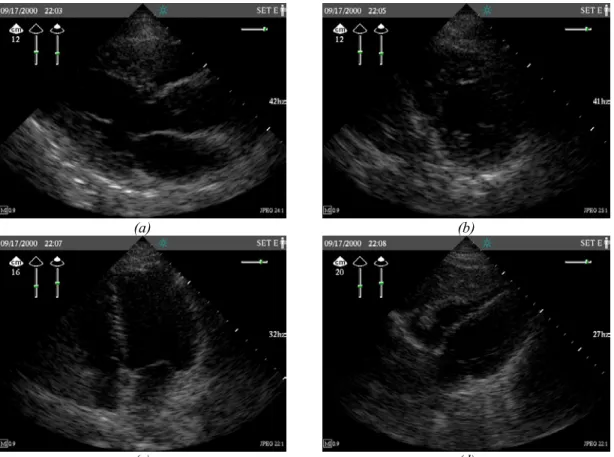
(a) (b)
(c) (d)
Fig. 2-1. Good quality typical cardiac ultrasound images. (a) Parasternal long axis (PLX) view. (b) Short
axis (SAX) view. (c) Apical four chamber (A4C) view. (d) Subcostal (SBC) view.
A completely automatic view matching algorithm would first have to determine the intended view of the input image data, and then set gains to drive the input data towards some target ideal data for the given view. The algorithm would also have to contain the target ideal data for the various views. To determine the feasibility of such an approach in real time, three tasks must be assessed. First, is it possible to determine the view of an input image using simple image statistics? Next, how likely is it that a target ideal data set can be determined for each view, and if so, how would the ideal data set be defined? Finally, if the view is known and a target data set is available, can matching the input data set to the target data set produce acceptable results?
2.2. Data Collection
To answer the first two questions, several sets of acoustic data were collected for analysis from Agilent Technologies’s portable ultrasound device using manual gain settings. For each data set, an experienced sonographer performed the imaging, including setting the gain parameters. The data collected represents the digitized acoustic samples just prior to scan conversion. Each sample can take on an integer value from 0 (48 dB) to 255 (96 dB). Three sets of data were used for this portion of the analysis: Set A (“average”), Set D (“difficult”) and Set E (“easy”). Set A includes one frame’s worth of acoustic data (121 lines of 480 samples each) for each of the four major views at high, low and good gain. The subject was a medium-frame female.
For Sets D and E, instead of recording each sample’s value, frequency of value
occurrence was recorded for several blocks of data. The acoustic data set was split into 4 lateral bands (of 30 or 31 lines each) and 4 radial bands (of 120 samples each), resulting in 16 blocks of 3600 or 3720 samples each. Sample values were considered in bins of 8, so that the number of samples having a value from 0-7, 8-15, etc. was recorded for each block. This procedure was used to speed up data collection from the ultrasound device. Sets D and E contain these frequency of occurrence data for five different frames of each of the four standard views taken at good gain settings. The subject for Set D was a large-frame, difficult to image male, and the subject for Set E was a medium-large-frame, easy-to-image female.
2.3. View Identification
The success of a view matching AGC algorithm depends on its ability to determine the view of the input frames. Data Set A was analyzed to examine the feasibility of performing view identification with simple, statistical techniques. Fig. 2-2 shows the frequency of occurrence histogram for the good manual gain settings frames in Set A. Acoustic value bins of size 8 were used to generate the histogram. The histograms for each of the four views are fairly similar, indicating that, at first glance, histogram identification will not be a feasible method of differentiating the views.
Fig. 2-3a and b show a similar set of histograms, this time focusing only on the data samples in the center 25% of the image. The top of an image sector and the edges all exhibit relatively high amounts of noise, so the center of the image is generally the “sweet spot” that contains the most important information in the frame. This figure shows that, when concentrating on the most important part of the image, the acoustic value content does differ significantly from view to view. Fig. 2-3a illustrates this observation overall, and Fig. 2-3b, showing the same histogram on a logarithm scale, highlights it for high acoustic values.
While these data are promising, it is necessary to keep in mind that the input to an AGC algorithm will probably not have good gain settings already applied to it—the real task is to identify a view even if the applied gains are off of the ideal value. Fig. 2-4a-d show the acoustic values histogram for high, low and good gain settings frames for each of the
four views. These histograms vary greatly within each view for different gain settings. Thus, histogram identification is not a viable technique for identifying the view.
0 1000 2000 3000 4000 5000 6000 7000 8000 0 8 16 24 32 40 48 56 64 72 80 88 96 104 112 120 128 136 144 152 160 168 176 184 192 200 208 216 224 232 240 248 Value F req u e n cy ( L in ear S cal e) PLX (Good) SAX (Good) SBC (Good) A4C (Good) (a) 1 10 100 1000 10000 0 8 16 24 32 40 48 56 64 72 80 88 96 104 112 120 128 136 144 152 160 168 176 184 192 200 208 216 224 232 240 248 Value Fr equency ( Logar it h mi c Scal e) PLX (Good) SAX (Good) SBC (Good) A4C (Good) (b)
Fig. 2-2. Histograms showing the frequency of occurrence of acoustic values in a frame of acoustic data
for sample images from the four common views: PLX, SAX, SBC and A4C. (a) Linear scale. (b) Logarithmic scale.
0 500 1000 1500 2000 2500 3000 3500 0 8 16 24 32 40 48 56 64 72 80 88 96 104 112 120 128 136 144 152 160 168 176 184 192 200 208 216 224 232 240 248 Value Frequency (Li n ear S cal e) PLX (Good) SAX (Good) SBC (Good) A4C (Good) (a) 1 10 100 1000 10000 0 8 16 24 32 40 48 56 64 72 80 88 96 104 112 120 128 136 144 152 160 168 176 184 192 200 208 216 224 232 240 248 Value Frequency (Logari thmi c Scal e) PLX (Good) SAX (Good) SBC (Good) A4C (Good) (b)
Fig. 2-3. Histograms showing the frequency of occurrence of acoustic values in the center 25% of a frame
of acoustic data for sample images from the four common views: PLX, SAX, SBC and A4C. (a) Linear scale. (b) Logarithmic scale.
1 10 100 1000 10000 100000 0 16 32 48 64 80 96 112 128 144 160 176 192 208 224 240 Value Frequency PLX (Good) PLX (High) PLX (Low) (a) 1 10 100 1000 10000 100000 0 16 32 48 64 80 96 112 128 144 160 176 192 208 224 240 Value Fre que nc y SAX (Good) SAX (High) SAX (Low) (b)
1 10 100 1000 10000 100000 0 16 32 48 64 80 96 112 128 144 160 176 192 208 224 240 Value Fr equency A4C (Good) A4C (High) A4C (Low ) (c) 1 10 100 1000 10000 100000 0 16 32 48 64 80 96 112 128 144 160 176 192 208 224 240 Value Frequency SBC (Good) SBC (High) SBC (Low) (d)
Fig. 2-4. Histograms showing the frequency of occurrence of acoustic values for frames of acoustic data
for sample images generated with good, high and low gain settings. (a) PLX view. (b) SAX view. (c) A4C view. (d) SBC view.
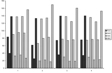
0 20 40 60 80 100 120 140 160 180 1 2 3 4 Radial Band Mean PLX SAX A4C SBC
Fig. 2-5. The means for the Set A data by radial band (1 corresponds to the top fourth of a sector; 4
corresponds to the bottom fourth of a sector). For each view (PLX, SAX, A4C and SBC), the good, low then high gain radial band means are plotted.
Another approach is to look at relative means. As seen in Fig. 2-5, the means for frames in a given view with differing gain settings vary differently. One hypothesis is that the means of each radial band relative to the overall mean of the frame may have better correlations. This hypothesis assumes that the effect of the gain is linear for all samples. Fig. 2-6 shows the relative mean data.
-20 -15 -10 -5 0 5 10 15 20 1 2 3 4 Radial Band Relat ive M ean PLX SAX A4C SBC
Fig. 2-6. The radial band means relative to the overall mean for the Set A data (radial band 1
corresponds to the top fourth of a sector; 4 corresponds to the bottom fourth of a sector). For each view (PLX, SAX, A4C and SBC), the good, low, then high gain radial band relative means are plotted.
Although some correlations exist, such as bands that are lower than the overall mean at one gain setting, are generally lower at other gain settings also, the relationship is not quantitative. Nevertheless, some heuristics may be applied to differentiate views using simple image statistics; for example, parasternal long axis and short axis views have bright third bands, while the apical four chamber view has a dim third band. The parasternal long axis and short axis views have negative relative means for the second band, which the other two views have positive relative means for this band. The
similarity of the parasternal long axis and short axis mean and relative mean data suggest that similar gain profiles can be applied for both of these views. It seems possible that views may be differentiated with simple statistical techniques such as looking at local means and relative means. It must be noted that these observations only hold for one patient, and whether these characteristics hold between views from different patients is addressed in the next section.
2.4. Determining Ideal Data Sets
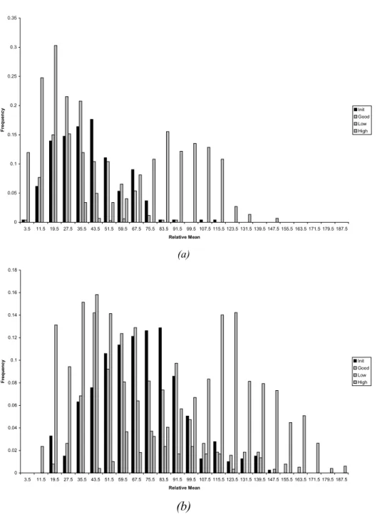
A target ideal data set for a given view must be acceptable for any patient. The data from Sets D and E were analyzed to see the degree of similarity between different frames of the same view in one imaging session (“study”), and between frames of the same view in different patients. Fig. 2-7a shows a plot of the frequency of occurrence of the acoustic values for each of the Set E frames. Fig. 2-7b is a similar plot for the Set D data set. Both of these plots demonstrate that even in one study, the frequency of occurrence of high acoustic values differs significantly within a view. As seen in Fig. 2-7b, for a difficult to image patient, the variation in the frequency of occurrence between frames of
the same view is comparable to the variance in the frequency of occurrence between frames of different views, at acoustic values above 200.
1 10 100 1000 10000 100000 0 50 100 150 200 250 Acoustic Value (0-255) Fr equency ( Logar it h mi c Scal e) PLX SAX A4C SBC (a) 1 10 100 1000 10000 100000 0 32 64 96 128 160 192 224 256 Acoustic Value (0-255) Fr equency ( Logar it h mi c Scal e) PLX SAX A4C SBC (b)
Fig. 2-7. A plot of the frequency of occurrence of pre-dynamic-range-mapped acoustic values for frames
of ultrasound data with different views (PLX, SAX, A4C, SBC), on (a) an easy-to-image patient and (b) a difficult-to-image patient. Data from five image frames for each patient-view combination is displayed.
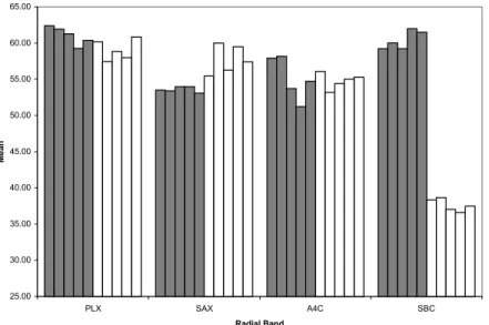
The frequency of occurrence of acoustic values for frames of the same view differ between patients as well. This observation is best illustrated by comparing the mean acoustic value of the Set E and Set D frames, shown in Fig. 2-8. Since exact sample values were not available, means were approximated by assigning the median value of a bin to each sample in that bin, (e.g. all samples in the 0-7 bin would be assumed to have a value of 3.5). Although for the long axis, short axis and four chamber views the mean values do not vary greatly between the two patients, the mean value is dramatically lower for Set D subcostal view frames compared to Set E frames. The mean acoustic values of the samples from the center 25% of all the images (samples in both the second or third lateral band and the second or third radial band) from Set E and Set D are graphed in Fig. 2-9. Fig. 2-9 shows that once the common edge noise is removed from consideration, the mean varies more between frames and between patients.
0 10 20 30 40 50 60 PLX SAX A4C SBC Radial Band M ean
Fig. 2-8. The overall pre-dynamic-range-mapped acoustic value means for five frames each of different
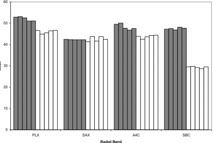
25.00 30.00 35.00 40.00 45.00 50.00 55.00 60.00 65.00 PLX SAX A4C SBC Radial Band M ean
Fig. 2-9. The center 25% pre-dynamic-range-mapped acoustic value means for five frames each of
different views (PLX, SAX, A4C, SBC) on an easy-to-image patient (gray) and a difficult-to-image patient (white). 0 20 40 60 80 100 120 All 1 2 3 4 Radial Band Mean 0 10 20 30 40 50 60 70 80 90 All 1 2 3 4 Radial Band M ean (a) (b) 0 10 20 30 40 50 60 70 80 All 1 2 3 4 Radial Band M ean 0 10 20 30 40 50 60 70 All 1 2 3 4 Radial Band M ean (c) (d)
Fig. 2-10. Acoustic means for an entire frame’s worth of acoustic samples, as well as by radial band (1
corresponds to the top fourth of a sector; 4 corresponds to the bottom fourth of a sector), for (a) PLX, (b) SAX, (c) A4C and (d) SBC views on an easy-to-image subject (gray) and a difficult-to-image subject (white). Data from five frames for each subject/view combination is shown.
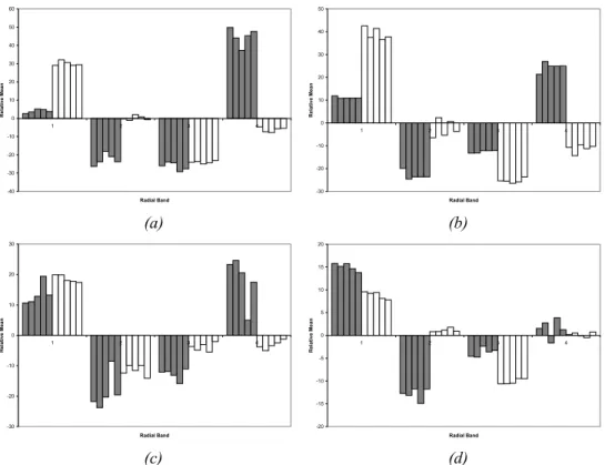
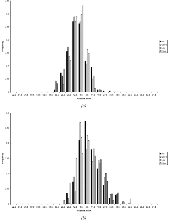
-40 -30 -20 -10 0 10 20 30 40 50 60 1 2 3 4 Radial Band Re la tiv e M e a n -30 -20 -10 0 10 20 30 40 50 1 2 3 4 Radial Band Re la tiv e M e a n (a) (b) -30 -20 -10 0 10 20 30 1 2 3 4 Radial Band R e la ti ve M e an -20 -15 -10 -5 0 5 10 15 20 1 2 3 4 Radial Band R e la ti ve M ean (c) (d)
Fig. 2-11. Acoustic means for a frame’s worth of acoustic samples, by radial band (1 corresponds to the
top fourth of a sector; 4 corresponds to the bottom fourth of a sector), for (a) PLX, (b) SAX, (c) A4C and (d) SBC views on an easy-to-image subject (gray) and a difficult-to-image subject (white). Data from five frames for each subject/view combination is shown.
Although the mean for some of the views is similar between subjects, it is necessary to examine the means by radial band as well. Knowing the ideal overall mean for a view only allows the development of an algorithm that can adjust the overall gain, but TGC settings operate at a finer granularity. Fig. 2-10 presents acoustic value means by radial band for all the frames in Set E and D. Here the difference in content of the easy-to-image patient easy-to-images and the hard-to-easy-to-image patient frames is even more apparent. The variation between frames of the same study is slight, but the variation between frames of different patients is much more marked. Even the relative brightness of each radial band is significantly different. Fig. 2-11 shows the radial band means relative to the overall mean by subtracting the overall mean for the frame from each of the radial band means.
These graphs clearly show that the brightest band differs from frame to frame. For example, for the parasternal long axis view the fourth radial band for Set E clearly has the highest mean, but the first radial band has the highest mean in the Set D data. This observation can be made for each of the views. Thus, a view cannot be characterized simply by its radial band means.
2.5. Performance of Parasternal Long Axis View Matching Algorithm 2.5.1. Algorithm Design
Despite the unencouraging results of the previous data analysis, a small study was conducted to assess the potential performance of a view matching algorithm if view identification and capture of a target “ideal” data set could be achieved. The chosen view to test was the parasternal long axis view. The entire acoustic sample data from a 12 cm depth parasternal long axis image of a medium-framed female was used as the target data. Gains were selected to minimize some error function between the input and target data.
For each frame of data, the algorithm calculates the mean. If the change from the previous frame’s mean is greater than a threshold of 5% of the previous mean, then the gains are left unadjusted. Otherwise, gain profiles are calculated that minimize the chosen error function and are applied to the next frame. Thus, this algorithm assumes that the transducer does not shift greatly from frame to frame and that the content from frame to frame does not change much. These assumptions are quite valid since the frame rate is around 30 Hz. The algorithm also assumes that the overall mean does change significantly when the transducer is taken on and off the body. Thus, one feature of this
algorithm’s design is that once the transducer is moved onto to the body, the mean change triggers the AGC mechanism and the gain change is immediate.
2.5.2. Gain Profile Application
For any given error function, several different methods of applying gain were
implemented. The first two methods compute the error for n bands and determine the appropriate gain value for each of these bands. n+1 points are then considered: the top of the sector, the bottom of the sector, and the n-1 points between 2 adjacent bands. The top and bottom are assigned the first and nth gain values respectively. The other points are assigned the average of the gain values of the bands directly above and below them. The gains for other samples are linearly interpolated between these points so that the applied gain profile is smooth. The first method uses n = 8 bands. The second method uses n = 28 bands, and adds to the computed gain profile the appropriate existing probe compensation curve gain values (these are empirically determined values that compensate for transducer characteristics).
The third method uses the bottom third of the image to determine an overall gain value, and the top third of the image to determine the near gain. These values are passed on to the existing TGC calculation algorithm in the system, which uses overall and near gain values and probe compensation curves.
2.5.3. Error Functions
Two error functions were considered. The first is a simple mean square error function, that, for the region being considered, compares each sample in the input data to its
corresponding sample in the target data set (since the sample values are on a logarithmic scale, applied gains are additive):
∑
= − + = N i i i N x G y error 1 2 1 ( ) ,where N is the number of samples in the region being considered, xi and yi are
corresponding samples in the current and target acoustic data sets respectively, and G is the gain to be applied to the region.
Since there may easily be a transducer shift corresponding to a few pixels, so the second error considers the square of the error between the means of two corresponding blocks of data. For each band, the data is split in four approximate equal blocks. The mean of each input data block is compared to the mean of the corresponding block in the target data:
2 1 1 1 (
∑
( )∑
) = = − + = N i i N i i N x G y error ,where N is the number of samples in the region being considered, xi and yi are
corresponding samples in the current and target acoustic data sets respectively, and G is the gain to be applied to the region.
It can be shown that the first error function is minimized if
∑
= − = N i i i N y x G 1 1 ( )It can also be shown that the second error function is minimized if
∑
∑
− = = N i i N i i N y x G ( ) 1 1Since the input data already has some gain applied to it from the previous iteration of the algorithm, G here represents the gain change to be applied.
2.5.4. Results and Discussion
Sample results of the six algorithms (3 gain profile applications each tested with the 2 error functions) are shown in Fig. 2-12a-f. The subject imaged was a small-framed female. The screen shots show the first two gain profile application techniques grossly overfit the data; there is an artificial bright band three-fourths of the way down the image, corresponding to the spectral reflection of the parasternum seen in a typical parasternal long axis view. Even with the second smoothing error function, the bright artifact still occurs. The third gain profile application method works much better, since it considers a larger number of samples in the calculation of each gain parameter.
Nevertheless, performance of this algorithm using either of the error functions was not very consistent; it stabilized at extremely different gain settings when the experiments were repeated.
The chief reasons for poor performance are probably the overfitting due to so many bands, and the use of an inappropriate representation of the target data set. The relative success of the last gain profile application method, however, underscores the fact that achieving acceptable AGC is much likelier if only a few gain parameters are set. By virtue of the fact that the first error function tries to match sample for sample, overfitting is a very predictable behavior of these algorithms. The target data set used captures all the details of a sample long axis image, instead of just the salient features that hold from
image to image. Given the lack of correlation seen in the analysis of image data means, it seems improbable that a simple, generic representation of a view can be captured.
(a) (b) (c) (d) (e) (f)
Fig. 2-12. Sample results of imaging the parasternal long axis view on a small-framed female
subject using view-based AGC. (a) Algorithm using the mean square error on 8 radial bands. (b) Algorithm using the mean square error on 28 radial bands and using probe compensation. (c) Algorithm using the mean square error to set the overall and near gains. (d) Algorithm using the square mean error on 8 radial bands. (e) Algorithm using the square mean error on 28 radial bands and using probe compensation. (f) Algorithm using the square mean error to set the overall and near gain.
One reason for this difficulty is the inherent fact that each patient is a different size. Although the maximum depth of interrogation can be adjusted to put the observed organ at approximately the same location on the screen, the discreet depths available and the different proportions of the heart (due to different inherited physiologies and different health conditions) make each individual patient’s images quite different. In light of these experiments with a view-based algorithm, an AGC algorithm that operates independently of view seems more promising. Such a generic algorithm can also perform on
non-standard views, which are highly likely to occur given an inexperienced sonographer who is simply trying to view the heart from any angle. The remainder of this thesis discusses the development and performance of such a generic AGC algorithm.
Xk; Rhap uhk;
3. Correlating Mean and Blood/Tissue Composition
3.1. Motivation for Correlating Mean and Blood/Tissue Composition To design an algorithm that sets gain values based on the composition of the input image requires an analysis of acoustic data to determine which parameters are useful in
determining the composition of an image. Since the AGC algorithm being designed must be implemented in real time, only computationally simple parameters can be considered. This chapter describes an investigation into the correlation between acoustic data means and blood/tissue composition; the next chapter discusses a similar investigation into the correlation between acoustic data variance and blood/tissue composition.
Theoretically, each sample in the acoustic data set for one frame could be classified as blood or tissue, in the style of rational gain compensation. The primary problem with such an approach is that from frame to frame, a sample in the same line and depth could change its composition, because of the motion of the heart. Thus, gain values for a particular sample could not be carried over from frame to frame. Hardware changes could be made to apply the gain to the current sample being analyzed, but given the architecture of the portable ultrasound device, such fine control is not possible through software. Changing the gain profile for each line is a time-consuming hardware
operation and would reduce the frame rate. Thus, the goal is to control automatically the manual time gain compensation (TGC) settings, and not operate on a line-by-line basis.
This consideration suggests that a block of acoustic data samples be considered together. Since gains are only being set in the radial direction, the first approach would be to group
the data in radial bands. The composition of samples varies from line to line, so
classifying an entire radial band as blood or tissue is virtually impossible. A more viable approach is to divide the acoustic data into r radial bands and l lateral bands, and each block of this matrix could be classified as mostly blood or tissue, by looking at all the acoustic samples in the block. Gains could be set to optimize the appearance of a majority of blocks.
Useful image statistics must be found to classify and optimize blocks of the image. We must be able to classify a block as blood or tissue, and then we must be able to define the desired appearance of a block based on its classification. The simplest attribute to consider, the mean of the values in a block of samples, can potentially answer both these questions. The gains are set ultimately to bring the brightness of the image to a desired, uniform level. The average value of a block is potentially a very good measure of its appearance. Can we find an ideal target mean for a blood block or a tissue block?
Absolute means are not likely to be a good metric for classification, however; when gains are mis-set, the means of each block would be expected to be significantly different from the ideal means. One would reasonably expect, however, that the relative means would be similar across images. For example, even if the gains are set extremely high, blood samples should still have lower values that tissue samples, unless saturation occurs, which is highly unlikely for moderate preset gain levels. Thus, the mean of each block relative to the mean of the entire image may be a useful attribute to classify the block as
blood or tissue. These considerations motivate this analysis of the correlation between block means and blood/tissue composition.
3.2. Data Collection
The acoustic sample values can be collected from two different points in the processing chain shown in Fig. 3-1. One choice is after dynamic range mapping, where the acoustic sample values of 0 to 255 map to 48 to 96 dB (values above and below this range are clipped to the minimum and maximum values). The dynamic-range-mapped (“B” mode) values are the values input to the scan converter. Another choice is to use the
pre-dynamic-range-mapped (“A” mode) data, where the acoustic sample values of 0 to 255 map to 0 to 96 dB. Thus, the samples that show up as blood (value = 0) in the dynamic-range-mapped-data occupy half the value range before dynamic range mapping. The means of the samples can be calculated using the data from either of these points, and both were considered.
AGC Alg. “B” data 121 lines of 480 samples 0 - 255 => 48 - 96 dB Signal from transducer Variable Gain and Clip A/D Conv. Dynamic Range Mapper Scan Conv. Display “A” data 121 lines of 480 samples 0 - 255 => 0 - 96 dB
Fig. 3-1. Selected features of the ultrasound processing chain. The input data to the AGC algorithm can
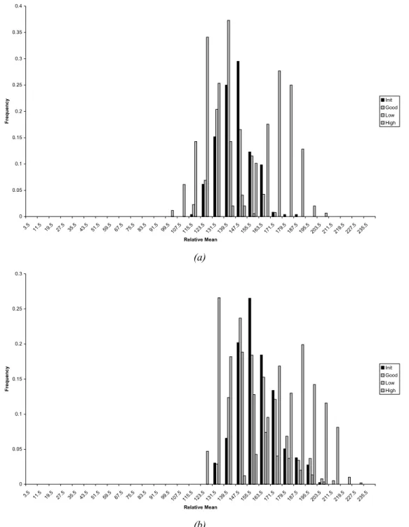
The data for this analysis came from Sets D and E (as described in Chapter 2), as well as Set F (“fine”), where data was collected in finer precision. To collect Set F data, an experienced sonographer performed the imaging, including setting the gain parameters. The data collected represents the digitized acoustic samples from both just before dynamic range mapping and just before scan conversion. Instead of recording each sample’s value, frequency of value occurrence was recorded for several blocks of data for Set F. The acoustic data set was split into 4 lateral bands (of 30 or 31 lines each) and 8 radial bands (of 60 samples each), resulting in 32 blocks of 3600 or 3720 samples each. Sample values were considered in bins of 8, so that the number of samples having a value from 0-7, 8-15, etc. was recorded for each block. Set F contains these frequency of occurrence data for five different frames of each of the four standard views taken at initial preset, good, low and high gain settings. The subject for Set F was a medium-frame, easy-to-image female. Each image corresponding to the data collected in Set D, E and F was split into 4 radial bands by 4 lateral bands (Sets D and E) or 8 radial bands by 4 lateral bands (Set F). Each of these block were hand-classified as blood or tissue.
3.3. Target Means for Blood and Tissue Composition 3.3.1. Target Dynamic-Range-Mapped Means
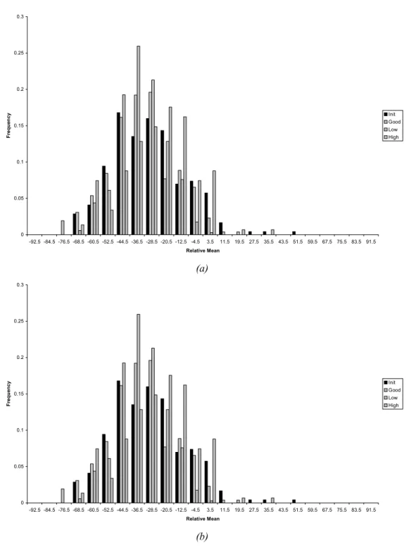
To arrive at target means for blood and tissue blocks, the frequency of means in hand-classified blood and tissue blocks from Set E, Set D and Set F data were examined. The number of blocks with means that fell in ranges of size 8 (i.e. 0-7, 8-15, etc.) were counted, and these counts were normalized over the total number of blocks. Fig. 3-2 shows the frequency of dynamic-range-mapped, “B” data means for blood and tissue blocks for Set E, Set D and Set E and D combined (blocks from a 4 x 4 grid). The
histograms show that whether dealing with a difficult-to-image patient (Set D) or an easy-to-image patient (Set E), the means for tissue and blood blocks fall in distinctly different ranges. The histograms also demonstrate the distribution of block means for different patients is fairly similar. The peak mean for blood blocks occurs between 24 – 32 for both Set D and Set E data. The peak mean for tissue occurs between 40 – 48 for Set D, and between 56 – 64 for Set E, and the second highest peak for the Set D tissue blocks also falls in the range of 56 - 64. The histograms illustrate that the range of means for tissue is much wider for tissue than for blood. More than 5% of the tissue blocks in both Set D and Set E data have means over 90. Looking at both sets of data together, blood means fall in a range of width approximately 70, whereas the tissue blocks fall in a range of width approximately 110.
0 0.05 0.1 0.15 0.2 0.25 0.3 0.35 0.4 3.5 11.5 19.5 27.5 35.5 43.5 51.5 59.5 67.5 75.5 83.5 91.5 99.5 107.5 115.5 123.5 131.5 139.5 Mean Fre que nc y Blood - D Blood - E Blood - Total Tissue - D Tissue - E Tissue - Total
Fig. 3-2. Frequency of occurrence of dynamic-range-mapped (“B” data) block means for blood and tissue
blocks for data generated with good gains settings on difficult-to-image (“D”) and easy-to-image (“E”) subjects.
0 0.05 0.1 0.15 0.2 0.25 3.5 11.5 19.5 27.5 35.5 43.5 51.5 59.5 67.5 75.5 83.5 91.5 99.5 107.5 115.5 123.5 131.5 139.5 147.5 155.5 163.5 171.5 179.5 187.5 Mean Fr equency Blood Tissue
Fig. 3-3. Frequency of occurrence of dynamic-range-mapped (“B” data) block means for blood and tissue
blocks for data generated with good manual gains (Set F data).
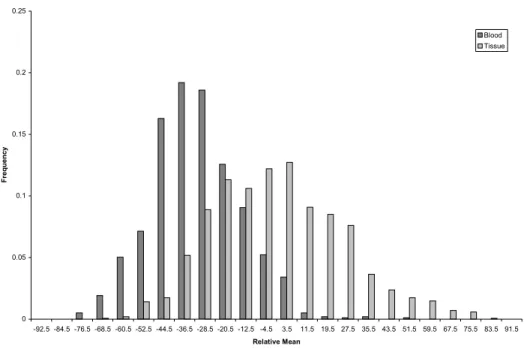
0 0.05 0.1 0.15 0.2 0.25 0.3 0.35 0.4 67.5 75.5 83.5 91.5 99.5 107.5 115.5 123.5 131.5 139.5 147.5 155.5 163.5 171.5 179.5 187.5 195.5 203.5 211.5 219.5 227.5 235.5 243.5 251.5 Mean Fr equency Blood Tissue
Fig. 3-4. Frequency of occurrence of pre-dynamic-range-mapped (“A” data) block means for blood and
tissue blocks for data generated with good manual gains (Set F data).
Fig. 3-3 shows a similar plot using dynamic-range-mapped “B” data from the good manual gain setting Set F blocks (from an 8 x 4 grid). Similar to the previous data, the
peak blood block mean occurs between 24 – 32, and the highest peaks for tissue blocks occur between 40 – 48, 64 – 72 and 56 – 64. The range of tissue means, approximately of a width of 150, is again much greater than the range of blood means, approximately of a width of 95.
3.3.2. Target Pre-Dynamic-Range-Mapped Means
Fig. 3-4 shows an identical plot using the pre-dynamic-range-mapped “A” data from the good manual gain setting Set F blocks. The peak blood mean, between 136 – 144, and the peak tissue mean, between 144 – 152, are much closer in value than the dynamic-range-mapped peak means. The range of tissue block means, approximately 85, is wider than the range of blood block means, approximately 60, and the frequencies of
occurrence fall off more slowly as values increase than as they decrease. The range widths for both blood block means and tissue block means are smaller than the corresponding range widths for the dynamic-range-mapped data.
3.3.3. Conclusions from Target Mean Analysis
Both the dynamic-range-mapped data and the pre-dynamic-range-mapped data analyses suggest that the blood block means should be around 52 – 53 dB and the tissue block means should be around 55-59 dB. Since the separation between the blood and tissue peak means is more pronounced in the dynamic-range-mapped data, it seems better to define the target means in terms of the dynamic-range-mapped scale. Fig. 3-2, 3-3, and 3-4, however, all show a significant overlap between blood and tissue block means. This overlap is probably due to the large block size. A block from 4 x 4 grid, or even an 8 x 4
grid, will most likely contain some samples that correspond to blood and some samples that correspond to tissue, making the composition of the block bimodal. During manual classification, there were several blocks encountered that were nearly blood and half-tissue. A smaller block size would increase the chance of having unimodal block
composition. As block compositions become more uniform, it would be expected that the target blood mean would lower and that the target tissue mean would rise.
Another practical consideration is to categorize tissue blocks into two more specific classes, ordinary tissue blocks, and specular tissue blocks, that would have higher means, due to the spread of tissue means. Blocks containing the specular reflections off the pericardium would be an example of “tissue” blocks that have unusually high means. Taking these observations and conjectures into account, a target blood mean (in terms of dynamic-range-mapped values) of under 32, a target tissue mean around 64 and a target specular mean over 90 are the suggested starting parameter values for a classification-based AGC algorithm.
3.4. Determining Blood and Tissue Composition from Normalized Means For the successful implementation of a classification-based AGC algorithm, it is
necessary to find attributes to aid in the classification of blocks of data in addition to defining the optimum appearance of each block. The normalized mean for each block, that is, the mean of each block relative to the overall mean of data set, is potentially a good attribute for classifying a block. Unless the gains cause the sample values to saturate, which is highly unlikely at usual gain levels, areas that should be dark in an