BIOGEOCHEMICAL APPLICATIONS OF COMPOUND-SPECIFIC RADIOCARBON ANALYSIS
By Ann Pearson
B.A., Oberlin College, 1992
Submitted in partial fulfillment of the requirements for the degree of Doctor of Philosophy
at the
MASSACHUSETTS INSTITUTE OF TECHNOLOGY and the
WOODS HOLE OCEANOGRAPHIC INSTITUTION October, 1999
@ Ann Pearson, 1999. All rights iserved.
The author hereby grants to MIT and WHOI the permission to reproduce and to distribute copies of this thesis document in whole or in part.
A Signature of Author:
Joint Program in Oceanography, Massachusetts Institute of Technology and Woods Hole Oceanographic Institution, October 1, 1999.
Certified by:_ _ _ __ _
Timothy I. Eglinton, Thesis Co-Supervisor
Certified by:
Ann P. McNichol, Thesis Co-Supervisor
A ccepted by: M arI et K . _Tivey MargA~et K. Tivey
Chair, Joint Committee for Chemical Oceanography, Woods Hole Oceanographic Institution.
MASSACHUSETTS INSTITUTE
BIOGEOCHEMICAL APPLICATIONS OF COMPOUND-SPECIFIC RADIOCARBON ANALYSIS
by Ann Pearson
Submitted on October 1, 1999, in partial fulfillment of the requirements for the degree of Doctor of Philosophy at the Massachusetts Institute of Technology and the Woods Hole
Oceanographic Institution
ABSTRACT
Compound-specific carbon isotopic (613C and A14C) data are reported for lipid
biomarkers isolated from Santa Monica Basin (SMB) and Santa Barbara Basin (SBB) surface sediments. These organic compounds represent phytoplanktonic, zooplanktonic, bacterial, archaeal, terrestrial, and fossil carbon sources. The lipids include long-chain n-alkanes, fatty acids (as FAMEs), n-alcohols, C3 0 mid-chain ketols and diols, sterols,
hopanols, and ether-linked C40-biphytanes of Archaea.
The data show that the carbon source for most of the biomarkers is marine euphotic zone primary production or subsequent heterotrophic consumption of this biomass. Two lipid classes represent exceptions to this finding. A14C values for the n-alkanes are consistent with mixed fossil and contemporary terrestrial plant sources. The archaeal isoprenoid data reflect chemoautotrophic growth below the euphotic zone.
The biomarker class most clearly representing marine phytoplanktonic production is the sterols. It is suggested, therefore, that the sterols could serve as paleoceanographic tracers for surface-water DIC.
The isotopic data are used to construct two algebraic models. The first calculates the contributions of fossil and modern vascular plant carbon to SMB n-alkanes. This model indicates that the A14C of the modern component is +235%o (post-bomb) or O%o
(pre-bomb). The second model uses these values to determine the origin of sedimentary TOC. The results are comparable to estimates based on other approaches and suggest that -60% of SMB TOC is of marine origin, modern terrestrial and fossil sources contribute -10% each, and the remaining -20% is of unknown origin.
ACKNOWLEDGEMENTS
I owe many thanks to the wonderful people who've made my graduate school experience some of the best years of my life.
Tim Eglinton continually gave me an empty slate and (seemingly) bottomless research budget. He let me take my research in any direction that was interesting and viable. Ann McNichol guided me through my first two years with patience,
thoroughness, and friendship. Despite his busy schedule, John Hayes always made time to allow me access to his mental encyclopedia. Phil Gschwend taught me that a dozen pages of verbal hand-waving is not as persuasive as a simple, quantitative argument. Thank you, all, for your encouragement and acceptance of nothing less than excellence.
This thesis also required the help of colleagues and friends beyond the
membership of my committee. Ellen Druffel organized the cruise in November 1996, on which I obtained the sediment samples. The Scripps Institution of Oceanography and the crew of R/V Roger Revelle generously donated their time and resources for two days of
sample collection in Santa Monica and Santa Barbara Basins. Every past and present member of the NOSAMS staff was critical to the completion of this project. Thank you especially to Bob, Karl, Al, Dana, and Sue for your flexibility and willingness to
accommodate all of my unusual requests. Without Bryan Benitez-Nelson, I probably would have succeeded in eventually blowing up the Fye lab - an extra-special thank you for the thousand small ways in which you helped out. Carl Johnson and Leah Houghton provided the irm-GCIMS data, including numerous re-runs and special requests; Rindy
Ostermann, Eben Franks, and Ellen Roosen helped with foraminifera samples.
This work was supported by National Science Foundation grants to T. I. Eglinton
(OCE-9415568, OCE-9809624, OCE-9708478), a National Institute of Standards and
Technology contract to T. I. Eglinton (43NANB615740), and the NOSAMS/National Science Foundation cooperative agreements (OCE-9301015, OCE-9807266). I received support from an MIT Ida Green Graduate Student Fellowship and a US EPA STAR Graduate Student Fellowship.
I thank my family for their unending support over the years. They've always encouraged me to do all the crazy things I ever wanted, including this. I thank Mom, especially, for being the first scientist in the family and Dad, for expecting me to grow up to be just like her. Dave, I always know you'll get it - thanks. To everyone in WHOI 94, thanks for the potlucks, parties, stress-relief, memories. Thank you to the 24 Millfield crowd, including honorary residents, for giving me a home away from home these last couple of years. Finally, thanks to the Cape Cod Women's Hockey League, I always had something fun planned on Saturday nights.
TABLE OF CONTENTS ABSTRACT...111 TABLE OF CONTENTS... vi TABLE OF FIGURES...x TABLE OF TABLES...xv CHAPTER 1 - INTRODUCTION... 17 1.1 INTRODUCTION...18 1.2 LIPID BIOMARKERS...20 1.3 CARBON ISOTOPES...21 1.3.1 13C Systematics 1.3.2 14C Systematics 1.4 GLOBAL AND LOCAL 14C DISTRIBUTIONS...29
1.4.1 Active Carbon Cycle 1.4.2 Bulk Reservoir Characteristics of 14C 1.4.3 Anthropogenic Perturbation of 14C Reservoirs 1.4.4 Santa Monica Basin (SMB) and Santa Barbara Basin (SBB) Field Sites 1.5 GOALS OF THIS THESIS... 50
1.6 REFERENCES... 51
CHAPTER 2 - GEOCHEMICAL METHODS... 55
2.1 BULK SAMPLES... 56
2.1.1 Samples 2.1.2 Bulk Sample Analyses 2.1.3 Foraminifera 2.2 ORGANIC GEOCHEMICAL METHODS...58
2.2.1 Lipid Analysis 2.2.2 High-Resolution Gas Chromatography (HRGC) 2.2.3 Gas Chromatography Mass Spectrometry (GC/MS) 2.2.4 Isotope Ratio Monitoring Gas Chromatography Mass Spectrometry (irm-GCIMS) 2.2.5 Preparative Capillary Gas Chromatography (PCGC) 2.2.6 Accelerator Mass Spectrometry (AMS) 2.3 REFERENCES... 69
2.4 APPENDIX... 71
2.4.1 SMB Bulk Core Data 2.4.2 PCGC Sample Log 2.4.3 Sample Recoveries and Fractionation 2.4.3.1 Organic Geochemical Procedures 2.4.3.2 PCGC Sample Recoveries CHAPTER 3 - MICROSCALE AMS 4C MEASUREMENT AT NOSAMS...83
3.2 M ETHODS ... ... -. ---87
3.2.1 HOxI and HOxII Standards 3.2.2 Hydrolysis of Carbonates 3.2.3 Combustion Blanks: JME and HOxI Powders 3.2.4 Graphite Preparation 3.3 RESULTS AND DISCUSSION ... 89
3.3.1 Optimization of Graphite Production Reaction 3.3.2 AMS Performance of Small Samples 3.3.3 Compensation for Machine-Induced Fractionation: Accuracy of HOxI and HOxII fm Results 3.3.4 Contribution of Background Carbon in the Analysis of Small Samples 3.3.4.1 Machine or Source Blank 3.3.4.2 Graphitization Blank 3.3.4.3 Combustion Blank 3.4 CONCLUSIONS ... 104 3.5 REFERENCES ... 107 3.6 APPENDIX...--109 3.6.1 Erratum, Figure 2.1 3.6.2 Further Characteristics of Graphite Production on Cobalt Catalyst 3.6.3 Isotopic Fractionation Effects During Incomplete Graphitization 3.6.4 Accelerator Performance for Multiple Small Sample Wheels CHAPTER 4 - AN ORGANIC TRACER FOR SURFACE OCEAN RADIOCARBON... 119
4.1 INTRODUCTION ... 120
4.2 RESULTS AND DISCUSSION... 123
4.2.1 B ulk Sam ples... 123
4.2.1.1 Surface Ocean A14CDc Record 4.2.1.2 Core Chronologies 4.2.1.3 SMB Sediment Core A1 4C: Foraminifera and TOC 4.2.1.4 Selection of Intervals for Compound-Specific Isotope Analysis 4.2.2 Organic Geochemical Analysis... 135
4.2.2.1 Sterol Lipid Fractions 4.2.2.2 PCGC Separations 4.2.3 Radiocarbon A nalysis... 144
4.2.3.1 Sterol A14C Data 4.2.3.2 Discussion 4.2.3.3 Factors Affecting 14C Isotopic Variability 4.2.4 Stable Isotope Analysis... 155
4.2.4.1 irm-GC/MS Data 4.2.4.2 Discussion: C26-C28 Sterols 4.2.4.3 Discussion: C29 Sterols and Dinosterol 4.2.5 Fraction of Allochthonous Organic Carbon in SMB Sediment... 164
4.3 CONCLUSIONS-... ... 168
4.4 REFERENCES... 170
4.5 APPENDIX... ... 177 4.5.1 Additional SMB bulk core data
4.5.2 13C-Fractionation During Reaction of Alcohols with Acetic Anhydride
4.5.3 S3C Comparison for PCGC Samples: Combusted CO2 and irm-GCIMS Data
4.5.4 A14C Comparison vs. Sample Size
CHAPTER 5 - RADIOCARBON EVIDENCE FOR AUTOTROPHIC
METABOLISM IN MARINE PLANKTONIC ARCHAEA... 191
5.1 INTRODUCTION... 192
5.2 RATIONALE AND APPROACH... 196
5.3 RESULTS... 197
5.4 DISCUSSION... 205
5.4.1 Radiocarbon Data 5.4.1.1 Data Comparison 5.4.1.2 DOC Incorporation Model 5.4.1.3 DIC Incorporation Model 5.4.2 Energy Source for Chemoautotrophy 5.4.3 Enzymatic Pathway of CO2 Fixation 5.5 CONCLUSIONS... 215
5.6 REFERENCES... 216
CHAPTER 6 - ORIGINS OF LIPID BIOMARKERS IN SANTA MONICA BASIN SURFACE SEDIMENT: A CASE STUDY USING COMPOUND-SPECIFIC "C AND 1 4C ANALYSIS ... 221
6.1 INTRODUCTION... 222
6.2 RESULTS ... 224
6.2.1 Bulk Core D ata... 224
6.2.2 Organic Geochemical Analysis.. ... 227
6.2.2.1 Selection of Intervals for Compound-Specific Isotopic Analysis 6.2.2.2 n-Alkanes 6.2.2.3 Fatty Acid Methyl Esters (FAMEs) 6.2.2.4 Alcohols 6.2.2.5 Diols and Archaeal Ether Lipids 6.2.3 PCGC Separations...244 6.2.4 A14C D ata...248 6.2.4.1 n-Alkanes 6.2.4.2 FAMEs 6.2.4.3 n-Alcohols, C3o-alkan-15-one-J-ol, and C30-alkan-1,15-diol 6.2.4.4 Sterols 6.2.4.5 Hopanols 6.2.4.6 Archaeal Lipids
6.2.4.7 Measurement Errors: Replicates and Recovery Standards
6.2.5 813C D ata... 260
6.2.5.1 n-Alkanes 6.2.5.2 FAMEs 6.2.5.3 n-Alcohols and Alkan-15-one-J-ols 6.2.5.4 Sterols and Hopanols 6.2.5.5 Archaeal Lipids and Alkan-1,15-diols 6.3 DISCUSSION... 274
6.3.1 Multi-Dimensional Carbon Isotope Distribution(s): 813C, A'4C, and A(A1 4C)... 274
6.3.2 Sources of Lipid Biomarkers to SMB Sediment... 278
6.3.2.1 FAMEs 6.3.2.2 Sterols and Hopanols 6.3.2.3 n-Alcohols, Alkan-15-one-J-ols, and Alkan-1,15-diols 6.4 SYNTHESIS AND CONCLUSIONS... 289
6.5 REFERENCES... 291
CHAPTER 7 - MODELS FOR THE ORIGIN OF N-ALKANES AND TOTAL ORGANIC CARBON IN SANTA MONICA BASIN SURFACE SEDIMENT... ... 297
7.1 INTRODUCTION...298
7.2 ISOTOPIC DATA... 300
7.2.1 TOC 7.2.2 n-Alkanes 7.3 N-ALKANE MIXING MODEL... ... 304
7.3.1 Quantitative Approach 7.3.2 Results and Discussion 7.3.3 Comparison to 2-Component n-Alkane Model 7.4 TOC MODEL... 323
7.5 SYNTHESIS AND CONCLUSIONS...331
7.6 REFERENCES... 333
CHAPTER 8 - CONCLUSIONS AND FUTURE WORK...337
8.1 CONCLUSIONS OF THIS THESIS... 338
8.1.1 Quality Control for Small Sample AMS 8.1.2 Phytoplanktonic Tracer Suitable for Paleoceanographic Applications 8.1.3 Exploration of Prokaryotic Metabolism 8.1.4 Sources of Lipid Biomarkers to SMB Sediment 8.1.5 Terrigenous Component of Continental Margin Sediments 8.2 FUTURE WORK... 344
Table of Fi2ures
Figure 1.1 Example structures of lipids discussed in this thesis... ... 21
Figure 1.2 Major global reservoirs involved in the active production, exchange, and cycling .... ... 31
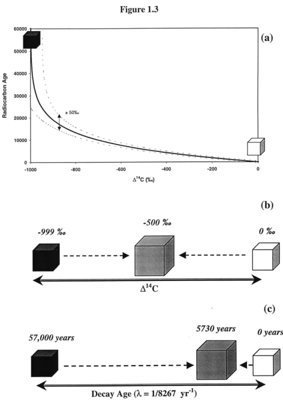
of organic carbon, based on Siegenthaler and Sarmiento (1993) and Hedges and Oades (1997). Reservoir sizes are shown in Gt carbon (1 GtC = 1015 gC). Numbers in parentheses are based on 1980s values; numbers without parentheses are estimates of the pre-anthropogenic values. Fluxes primarily mediated by biological reactions are shown with dashed arrows; physical transport processes are shown with solid arrows. Figure 1.3 (a) Decay age (1 = 1/8267 yr") as a function of A1 4C; (b) mixing equal proportions... ... 36
of modern and "dead" material yields A14C = -500%o; while (c) the "age" is not equal to what would be considered a linear average of the ages of the two materials. Figure 1.4 Evolution of atmospheric C02, Southern California Bight surface water DIC, and.... ... 38
Santa Monica Basin surface sediment TOC A14C values since 1950. The atmospheric A14C record is based on the figures and references in Broecker and Peng (1982) and Hesshaimer et al. (1994); the surface water DIC record is based on references in Robinson (1981), Williams et al. (1992), and this thesis; the TOC record is from this thesis. Figure 1.5 Santa Monica Basin core location for this thesis: 33'44.00' N, 118*49.99' W ... ... 39
905 m depth, using an Ocean Instruments® Multicorer, November, 1996, R/V Roger Revelle, cruise Pulse-32. Figure 1.6 Santa Barbara Basin core location for this thesis: 34*13.5' N, 120*03.5' W, ... 40
595 m depth, using an Ocean Instruments® Multicorer, November, 1996, R/V Roger Revelle, cruise Pulse-32. Figure 1.7 Pre-bomb A4C distribution in SMB; data from Table 1.6... ... 44
Figure 1.8 Post-bomb (1990s) A14C distribution in SMB; data from Table 1.6... 45
Figure 2.1 Schematic of the PCGC system... 66
Figure 2.2 SMB sedimentary S13CTOC, measured on splits of CO2 prepared by closed-tube ... ... 71
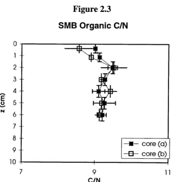
combustion. Figure 2.3 Organic C/N ratio in SMB sediment... 72
Figure 2.4 Total extractable lipids in SMB sediment...72
Figure 2.5 Percent organic carbon in SMB sediment.... ... 73
Figure 3.1 (a) Calculated error qFs for dilution to a conventional sample size of 500 ggC (A) ... 86
and for dilution to 100 ggC only (B). (b) Calculated error UFs for dilution of a l0pgC sample up to r = 10 using a variable qFx = 0.06e-0018Mx. Increased precision in UFx partially offsets the dilution error. Figure 3.2 (a) 23 factorial analysis of T, R, and H effects on reaction yield. (b) 24 factorial ... 92
analysis of T, R, H, and Q effects on reaction yield. A (+) indicates the upper range of the factor improves % yield, while a (-) indicates the lower range improves % yield. The variables are described in the text. Figure 3.3 Observations showing that the 12C current measured for small samples varies ... ... 93
with size, according to the approximate relationship 112=0.9M. M=mass of carbon in micrograms; 112 = 12C current in nanoamperes.
Figure 3.4 Dependence of the measured 1 4C/1 2C isotope ratios for (a) HOxI and (b) HOxII . 95 small samples on the generated 12C ion current. Ratios have been normalized to average values obtained for HOxI and HOxII standards of conventional size.
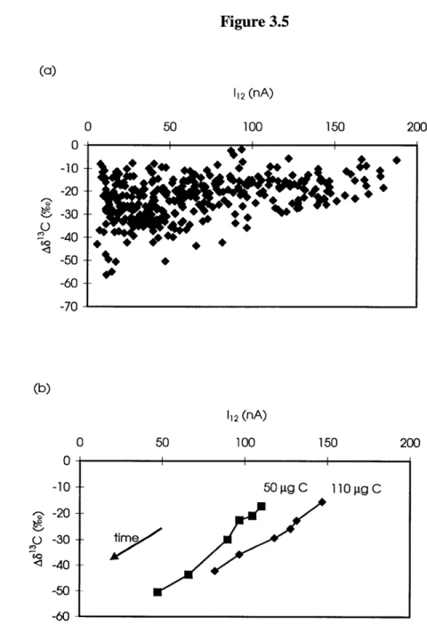
Figure 3.5 (a) 13C fractionation of HOxI and HOxII small samples as a function of the... ... 96 generated 1C ion current for all discrete time points. (b) A813C and I12 variation within
samples as a function of elapsed measurement time.
Figure 3.6 Results obtained for HOxI and HOxII small standards when fm values are ... ... 100 calculated relative to adjacent small standards of similar size. A = sample for which
Poisson error was used.
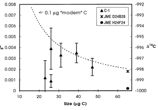
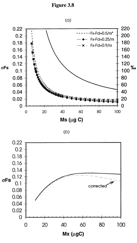
Figure 3.7 Graphitization blank as measured for IAEA C-I carbonate...102 Figure 3.8 (a) Re-calculated error aF, for dilution to a composite sample size of 100 gC, .... ... 110
shown for a range of assumed values of F,. (b) Re-calculated error oF, for dilution of a 10 ggC sample up to r, = 10, using a variable aF, = 0.06e-001Mx, assuming F, = 0.5.
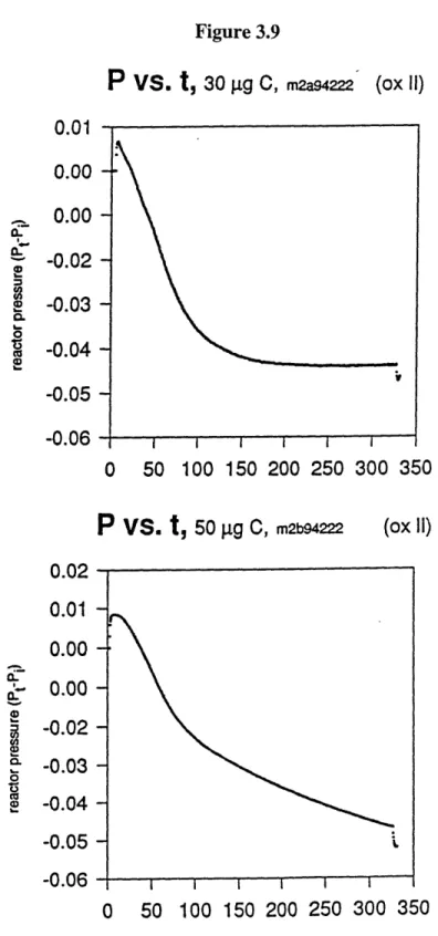
Figure 3.9 Pressure vs. time graphs for a graphite reaction achieving 85% yield (a) and for . 113 one reaching only 60% yield (b).
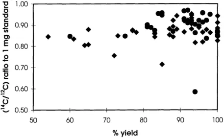
Figure 3.10 Isotope effects observed as a function of graphite reaction yield. HOxI, ... 115 diamonds; HOxII, circles.
Figure 3.11 (a) Cartoon of the decrease in 4C/'2C for a set of HOxI standards arranged in ... 117 order of decreasing I12. (b) Random insertion of samples between these standards.
(c) Samples and standards arranged in order of decreasing I12.
Figure 3.12 (a) Correlation between I12 and C/Co ratio for a small sample wheel. (b) The ... 118 same '12 data, plotted as a function of sample size (corrected for % yield).
Figure 4.1 Evolution of SCB surface water A1 4C through the twentieth century, showing the ... 126 Figure 4.2 Calendar year chronology of the Santa Monica Basin core used in this thesis as ... 128
determined by 210Pb dating. The core was sectioned at 0.75-cm intervals to 1.5 cm, then at 1.0-cm intervals to 8.5 cm.
Figure 4.3 Bulk sample A14C data for the SMB core. Foraminifera are shown in hollow ... 130 symbols (triangles, planktonics; circles and squares, benthics), TOC in solid diamonds,
and the surface water A14CDIC model created from literature data is shown as a dashed line. Figure 4.4 HRGC traces for the three sterol fractions selected for compound-specific ... ... 136
isotopic analysis. (a) SBB 0-1 cm, (b) SMB 0-0.75 cm, (c) SMB 4.5-5.5 cm, all derivatized to acetates for PCGC separation and 14C analysis; (d) SMB 4.5-5.5 derivatized to trimethyl-silyl ethers as was necessary for S13C analysis by irm-GCIMS.
Figure 4.5 HRGC traces for two 4-methyl-sterol fractions (as acetates) for PCGC separation ... 137 of dinosterol.
Figure 4.6 (a) Expanded C29 sterol region of the SMB 0 - 0.75 cm chromatogram originally ... 140 obtained by HRGC. (b) The mass 45/44 isotope ratio trace for the same region of this
sample has four clear peaks, and (c) the corresponding mass 44 ion chromatogram shows the improved peak separation obtained on the irm-GCIMS system.
Figure 4.7 HRGC traces of SMB 0 - 0.75 cm 4-desmethyl-sterol fraction. The original... 143 mixture is shown at the bottom. Re-analyzed aliquots of individual PCGC trap contents are shown above. Sterol isomer peaks are labeled as in Figure 4.4, and recovered quantities of the pure compounds are given.
Figure 4.8 Two-dimensional carbon isotope plot of sterol biomarkers, showing agreement of. 149 pre-bomb and post-bomb compound-specific A14C data with the record of surface water
A14CDIC- Surface water A14CDIC measurements are shown as solid lines; dashed lines represent planktonic foraminifera.
Figure 4.9 The effect of differing degradation rates on the measured A C of lipids having... 155 the same original source. (a) The A1 4C of the source material over time. (b) Compound
X degrades at 5 times the rate of compound Y. (c) The maximum difference between
measured A1 4C values occurs over the interval when the source A14C was changing most rapidly.
Figure 4.10 Comparison of 81 3C data for individual sterols from SMB and SBB sediments,...158 showing the similarity of the relative 13C distribution among the isomers studied.
Figure 4.11 Comparison of 1 3C data for individual sterols from the additional SMB ... ... 159 sedimentary horizons, 0.75 - 1.5 cm and 5.5 - 6.5 cm, for which 14C isotopic data were
not obtained.
Figure 4.12 The fraction of TOC in SMB sediment traceable to marine planktonic ... ... 168 production. The linear fit was determined for A14CToC relative to the A14CDIC model
derived from data in Table 4.1 (diamonds). The triangles show the agreement between sterol A14C data and the model solution.
Figure 4.13 Reaction mechanism and energy diagram for the formation of an acetate ... ... 179 derivative from an alcohol and isotopically heterogeneous acetic anhydride.
Figure 4.14 Sterols: 13
C difference between CO2 splits and irm-GCIMS data... ... 188
Figure 4.15 Sterols: A1 4C difference vs. 13C difference...189 Figure 4.16 The difference between individual A4
Csterol and A1 4CDIC as a function of ... 190 sample size. There is no uniform bias toward more negative or positive offsets for the
smaller samples, although there is more scatter observed.
Figure 5.1 (From DeLong et al., 1998) Phylogenetic division of the three Domains of life ... 193 including the division of Archaea into the two major Kingdoms, Crenarchaeota and
Euryarchaeota.
Figure 5.2 Structure of caldarchaeol, an ether-linked C80 isprenoid membrane lipid of ... ... 194 thermophilic and marine planktonic Archaea.
Figure 5.3 Structures of lipids used for compound-specific isotope analysis...198 Figure 5.4 Gas chromatograms of SBB 0-1 cm ether lipid fraction (as hydrocarbons). (a)...200
total mixture; (b) n-C33 standard as recovered by PCGC; (c) C40:2cy as recovered by
PCGC; (d) C40:3cy as recovered by PCGC; (e) FID output for total mixture during PCGC separation on the 1-m multi-capillary column.
Figure 5.5 A14C vs. 813C for sterols (crosses) and archaeal ether lipids, SBB 0-1 cm (circles),.. ... 204 SMB 5.5-8.5 cm (squares). Also included are solid lines showing the A C of surface
water DIC during the 1990s (upper line) and prior to atmospheric nuclear weapons testing (lower line).
Figure 5.6 Comparison of SMB and SBB A4CDIC and water column 02 and N0
2~ profiles...210
SBB is shown in the upper section of the figure, SMB in the lower section. Wide horizontal arrows point to the "14C-projection depths" of archaeal biomass production and the corresponding regions of the nutrient profiles.
Figure 6.1 Bulk sample A14C data for the SMB core. Bottom water A14
CDIC as recorded ... 226 by benthic foraminifera is shown as a thin solid line; the surface water A14CDIC model
created from literature data is shown as a dashed line. Sedimentary A14CTOC (diamonds) is intermediate between the two water mass records.
Figure 6.2 (a) Total aliphatic hydrocarbon fraction for SMB 0-2.5 cm sediment horizon ... 229 and (b) n-alkane fraction obtained following urea adduction of the same sample;
letters identify compounds collected by PCGC for 4C-AMS analysis (data in Table 6.2). Figure 6.3 Absolute and relative abundance of n-alkanes in SMB sediment... ... 230 Figure 6.4 (a) Total FAME plus ketone fraction for SMB 4.5 - 5.5 cm sediment horizon ... ... 233
(original chromatogram of SMB 0 - 0.75 cm fraction not available) and (b) purified FAME fraction from SMB 0 - 0.75 cm horizon; letters identify compounds collected
by PCGC for 14C-AMS analysis (data in Table 6.2).
Figure 6.5 Absolute and relative abundance of fatty acids (as FAMEs) in SMB sediment...234 Figure 6.6 (a) Total alcohols (as acetates) (Fraction 7) from the SMB 0.75 - 1.5 cm ... ... 237
horizon and (b, c) n-alcohol and non-adducted fractions obtained following urea adduction of the same sample; letters identify compounds collected by PCGC for
14
C-AMS analysis (data in Table 6.2).
Figure 6.7 Absolute and relative abundance of n-alcohols and C30-alkan-15-one-1-ol in... ... 238
SMB sediments. (7*n-C24 = seven times the abundance of n-C24; 6* n-C24= six times the abundance of n-C24.) Figure 6.8 4-Desmethyl-sterols (as acetates) (Fraction 8) from the SMB 0 - 0.75 cm ... ... 239
horizon; letters identify compounds collected by PCGC for 14C-AMS analysis (data in Table 6.2). Figure 6.9 Absolute and relative abundance of sterols and hopanols in SMB sediments...240
Figure 6.10 (a) Total diols and archaeal ether-linked isoprenoid lipids (Fraction 9) from ... 242
the SMB 0 - 0.75 cm horizon (not abundant enough for compound-specific 14C analysis) and (b) hydrocarbon fraction generated by HI cleavage and LiAIH4 reduction of SMB 5.5 - 8.5 cm Fraction 9; letters identify compounds collected by PCGC for 1 4C-AMS analysis (data in Table 6.2). Figure 6.11 Absolute and relative abundance of C30-alkan-1,15-diol and C40 isoprenoid ... ... 243
ether linked lipids of Archaea in SMB sediment. Figure 6.12 HRGC traces of SMB 0 - 0.75 cm FAME fraction. The original mixture is ... ... 245
shown at the bottom. Re-analyzed aliquots of individual PCGC trap contents are shown above. FAME isomer peaks are labeled as in Figure 6.4 and Tables 6.1 and 6.2, and recovered quantities of the pure compounds are given. Figure 6.13 irm-GCIMS data for SMB sediment n-alkanes. Dark colored bars indicate the ... 262
odd-chain n-alkanes, and colorless bars indicate the even-chain n-alkanes. Figure 6.14 irm-GC/MS data for SMB and SBB sediment FAMEs. The saturated fatty ... ... 264
acids, C12:0, C14:0, C16:o, and C18:0 are shown with black bars. The odd-chain, branched-chain, and unsaturated fatty acids are shown with colorless bars. Even-numbered, long-chain alkanes are shown with gray bars. Figure 6.15 irm-GC/MS data for SMB post-bomb sediment n-alkanols...266
Figure 6.16 irm-GCIMS data for SMB pre-bomb sediment n-alkanols...267
Figure 6.17 irm-GCIMS data for individual sterols from SMB and SBB sediments...269
Figure 6.18 irm-GC/MS data for sterols from the additional SMB sedimentary horizons,... ... 270
0.75 - 1.5 cm and 5.5 - 6.5 cm, for which 14C isotopic data were not obtained. Figure 6.19 irm-GCIMS data for Fraction 9, alkyl-1,15-diols and archaeal lipids... ... 273
Figure 6.20 A4 C vs. S13C distribution for SMB biomarkers. Post-bomb data (0-0.75,... 275
0.75-1.5, 0-2.5 cm horizons) are shown with solid symbols and pre-bomb data (4.5-5.5, 5.5-8.5, 2.5-7.5 cm horizons) with hollow symbols. A, n-alkanes; ., FAMEs; E, n-alcohols; +, sterols and hopanols; Y, archaeal lipids and C30-diol (post-bomb data from SBB 0-1 cm). Letters identify individual compounds as in Table 6.2. Figure 6.21 Three-dimensional plot of the post-bomb data presented in Figure 6.20. The... 277
z-axis shows the change in A14C recorded by individual biomarkers between pre-bomb and post-bomb horizons (A(A'4C)= A14Cpost-bomb - A14Cpre-bomb). The horizontal plane at A(A'4C) = +150%o represents the change in surface water A14CDIC over the same time interval. All of the analyzed lipids except n-alkanes and archaeal isoprenoids fall within ±30%o of this plane. Figure 7.1 Concentration distributions and S13C values of the three assumed n-alkane... ... 312
sources used to create the n-alkane mixing model. Figure 7.2 Results of the mixing model for SMB pre-bomb (2.5-7.5 cm) n-alkanes. (a) 8"C...313
data for n-C24 to n-C33 n-alkanes (squares) and 513C predicted by the best-fit model solution (bars). Residuals shown above are all < 1 .0%o. (b) A14C data for composite even numbered n-alkanes (n-C24+26+28+30), and individual n-C27, n-C29, and n-C31
alkanes (circles) and A14C for all n-C24 to n-C33 alkanes predicted by the best-fit model solution (bars).
Figure 7.3 Results of the mixing model for SMB post-bomb (0-2.5 cm) n-alkanes. (a) 1 3C...314
data for n-C24 to n-C33 n-alkanes (squares) and S13C predicted by the best-fit model
solution (bars). Residuals shown above are all < 1.0%o. (b) A14C data for composite even numbered n-alkanes (n-C24+26+28+30), and individual n-C27, n-C29, and n-C31
alkanes (circles) and A14C for all n-C24 to n-C33 alkanes predicted by the best-fit
model solution (bars).
Figure 7.4 Relative contributions of each of the three endmembers to the n-alkane ... ... 315 samples. The petroleum source is relatively more important in the 0-2.5 cm horizon,
terrestrial material is relatively enriched in the 2.5-7.5 cm horizon, and the shale fraction is the same in both. Agreement between the data and model is within 10% in the surface sediment and within 20% in the deeper sample.
Figure 7.5 A new representation of Figure 6.21. The A(A14C) values for the n-alkanes are... ... 320 replaced with the modeled result A(A14Ceresi) = +235%o. The horizontal plane at
A(A14C) = +150%o represents the change in surface water A14C since pre-bomb conditions. Figure 7.6 Matlab model solution for the fractional contributions of planktonic (P),...325
terrestrial (7), fossil (F), and unknown (U) carbon to SMB TOC.
Figure 8.1 Lipid classes distributed around a simplified phylogenetic "tree of life". ... 346 Phylogenetic tree from Schlegel, 1989.
Table of Tables
Table 1.1 Common source assignments of lipid biomarkers...20
Table 1.2 Equilibrium 1C fractionation effects, adapted from Hayes (1993) and Raven (1997)...23
Table 1.3 Kinetic fractionation effects associated with solute reactions and transport, adapted... ... 24
from Raven (1997). Table 1.4 Kinetic fractionation effects associated with enzymatic reactions, adapted from Bott...25
and Thauer (1989), Raven (1997), and specific references as noted below. Enzymes: Ribulose bis-phosphate carboxylase-oxygenase (RUBISCO), Phosphoenolpyruvate carboxylase (PEPC), Phosphoenolpyruvate carboxykinase (PEPCK), Pyruvate synthase (PS), a-Ketoglutarate synthase (KGS), Isocitrate dehydrogenase (IDH), Acetyl-CoA Carboxylase (AC), Propionyl-CoA carboxylase (PC). Table 1.5 Pre-industrial, pre-nuclear A14C and translated "decay ages" for bulk carbon ... ... 34
reservoirs. Also included are the expected ranges of S13C values for these carbon pools. The estimated ranges of A14C for soils are taken from Becker-Heidmann et al., 1996. Other references are from Lewan (1986); Emerson et al. (1987); and Druffel et al. (1992). Table 1.6 A14C distribution in the local environment of SMB. The SBB environment is ... 46
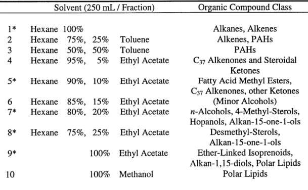
similar except for a shallower water column and less negative deep-water A CDIC value. Table 2.1 Flash SiO2-gel chromatographic separation of lipid biomarker classes... ....59
Table 2.2 Complete PCGC Sample Log... 74
Table 2.3 Recoveries and 13C fractionation for organic geochemical methods... 79
Table 2.4 Recoveries for PCGC samples as determined by various quantitation methods... 81
Table 3.1 Factorial Analysis Parameters ... 90
Table 4.1 A history of surface water A4CDIc, mollusc shell A1 4C, and pteropod A14C ... ... 125
measurements recorded in the SCB. Except for the 1996 sample (this study), the DIC data were previously gathered and published by Williams et al. (1992, and citations therein). The first three samples were collected off the Scripps Institution of Oceanography Pier (32* 52' N, 117*44' W); the fourth is a GEOSECS station (28*30' N, 121*29' W); the fifth is south of San Diego (31*9.9' N, 117 12' W); this sixth is from the central Santa Monica Basin. The mollusc shell data are from coastal California (33 - 38*N) and were reported by Robinson (1981). The pteropod value is from Santa Barbara Basin sediment with a calendar data 1920 AD (Baumgartner and Southon, 1996). Table 4.2 Isotopic data for bulk samples, SMB core...133
Table 4.3 Sterols identified in the chromatograms in Figures 4.4 and 4.5... ... 135
Table 4.4 Abundance of major sterols in SMB and SBB sediment samples... 138
Table 4.5 Isotopic data for individual sterols from SMB and SBB sediments...145
Table 4.6 Sources of A1 4C variability in phytoplanktonic biomarkers of common source...154
Table 4.7 irm-GCIMS 13 C data for all sterol peaks as identified in Figures 4.4 and 4.5. ... 157
Fractions were run in triplicate, and measurement precision is reported. The accuracy is estimated to be ±0.4%o. Table 4.8 irm-GCIMS 81 3C data for the additional SMB sedimentary horizons, 0.75 - 1.5 cm.... ... 157
and 5.5 - 6.5 cm, as determined for -OTMS ethers. Fractions were run in triplicate, and measurement precision is reported. The accuracy is estimated to be ±0.4%o.
Table 4.9 S13C data for bulk acetylation experiments and PCGC recovery standards...182
Table 4.10 Androstanol standard 81 3C measured by irm-GCIMS:... ... 184
AS1C = S1 Cmeasuret - (-33.3%o). Table 4.11 irm-GCIMS data for sterols run as acetates. The fractionation effect is always... ... 185
in the regular sense (products lighter than original substrate), but the magnitude is not constant between batches. Table 5.1 A14C data for individual lipids from surface and pre-bomb sediment horizons as...199
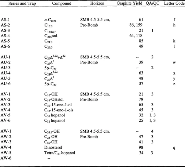
described in the text. Structures of compounds are shown in Figure 5.3. A dash indicates no value was determined. Table 6.1 List of individual compounds isolated by PCGC for which A14 C values were ... ... 247
obtained, in order of processing. Table 6.2 Summary of compound-specific A4 C and 83 C data. The 813C values are based...250
on irm-GC/MS measurements unless otherwise indicated. Table 6.3 Recovery standards and replicate measurements used to assess the quality of the...260
compound-specific A14 C data. Table 6.4 Sources of lipid biomarkers in SMB surface sediments... ... 290
Table 7.1 Sediment horizons as sectioned for the SMB core, the chronology determined ... 301
by 210Pb dating, and the associated A14CTOC values. Table 7.2 SM B n-alkane isotopic data...302
Table 7.3 Results of n-Alkane mixing model... ... 311
Table 7.4 Comparison of 2-component and 3-component n-alkane mixing models... ... 322
Table 7.5 Assumed A"C values used in the TOC mixing model...324
Table 7.6 TOC mixing model solution...326
Table 7.7 Comparison of the A1 4 C model with the results of other approaches to SMB ... ... 329 sedimentary TOC.
CHAPTER 1
1.1 INTRODUCTION
The total organic carbon (TOC) in marine sediments is a heterogeneous mixture of products derived from multiple sources. In most oceanic environments, the majority of TOC is believed to originate from autochthonous phytoplanktonic biomass and subsequent heterotrophic degradation of this material. Both open-ocean and continental margin sediments, however, also contain organic matter from other sources. Some fraction of TOC may be derived from land plant debris that spent significant time within terrestrial soils prior to erosion and deposition in marine sediments. Other carbon may come from weathered continental shales or ancient kerogen. Still other components of TOC could be derived from benthic chemoautotrophic processes, from in-situ bacterial production at sites of active petroleum or gas seeps, or from bacterial incorporation of refractory dissolved organic carbon (DOC).
Most of the allochthonous and chemosynthetic endmembers represent sources of organic carbon with lower radiocarbon (14C) concentrations ("older" radiocarbon ages)
than the fraction of TOC originating from phytoplanktonic production. The only
exception is the rapid transport and sedimentation of recently-synthesized terrestrial plant material, which will have a 14C concentration in equilibrium with atmospheric C0
2, making it "younger" than marine biomass. Some of the allochthonous components may represent carbon fixed in the past, but which spent time in an intermediate reservoir before being transported to marine sediments. This scenario has different implications for atmospheric CO2 concentration, carbon sequestration, and nutrient distributions than
the production of "old" biomass carbon by contemporary bacteria utilizing pre-aged carbon sources. Distinguishing between the different scenarios responsible for
contributing pre-aged carbon to marine sediments is important to a general understanding of the carbon cycle.
Isotopic analysis of individual lipid biomarker molecules can provide more information about the biogeochemical processes affecting marine sedimentary composition than bulk-phase isotopic measurements on TOC alone. The
compound-specific approach was initially developed for studies of the stable carbon isotope (13C)
distribution in lipids extracted from samples of modem and ancient geologic age (e.g. Freeman et al., 1990; Hayes et al., 1990), and it proved very useful as a tool to describe the diversity of these sources and the origins of specific biomarkers. More recently, Eglinton et al. (1996) developed a preparative capillary gas chromatographic (PCGC) separation method that is able to isolate lipids with sufficient purity and abundance for compound-specific 14C measurement by accelerator mass spectrometry (AMS). Using this approach, Eglinton et al. (1997) demonstrated a wide range of 14C ages within discrete sedimentary horizons from two separate environments. The data indicated that some co-occurring lipids either were formed at different times; or that the lipids were simultaneously biosynthesized, but utilized carbon source pools of differing initial isotopic composition. The implication of this work is that compound-specific 14C measurements may be used to distinguish biogeochemical pathways of carbon utilization
and transfer in a manner analogous to compound-specific 13C analysis.
The overall goal of this project was to generate the first detailed molecular-level radiocarbon data set for a comprehensive suite of lipid biomarker compounds. It
contributes to the general understanding of carbon cycle biogeochemistry and specifically examines some of the mechanisms responsible for contributing organic carbon of
non-marine photosynthetic source to ocean sediments. The study focuses on a 10-cm core from Santa Monica Basin, California, USA, and is supplemented by a core-top sample from the adjacent Santa Barbara Basin. These cores were chosen because of the resolution of the sediment records, the availability of ancillary data, and because on a radiocarbon time-scale, the samples are all "contemporary". The variability in biomarker
14C concentrations reflects differences in isotopic composition of the endmember sources
only, with minimal in-situ 14C decay. The primary tracer property of 14C utilized in this thesis is the increase in atmospheric 14C concentration caused by above-ground nuclear weapons testing in the 1950s and 1960s. This excess "bomb-14C" has invaded the modern surface ocean and terrestrial biota and allows the products of recent biological production to be identified easily. Pre-aged organic materials or biomass formed in
locations physically removed from the influence of atmospheric CO2 (i.e. the deep ocean) are distinguished by their lack of incorporation of bomb-14C.
1.2 LIPID BIOMARKERS
The organic matter in marine sediments consists of both recognizable biochemical constituents of organisms (carbohydrates, proteins, lipids, and nucleic acids), as well as more complex polymeric materials and non-extractable components (kerogen). Among the recognizable biochemicals, the lipids have a diversity of structures often assignable to specific biological sources. Lipids are also comparatively easy to analyze by gas
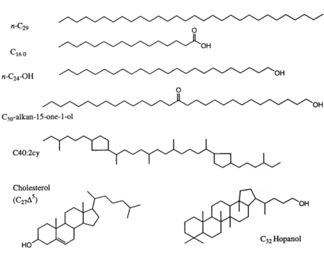
chromatographic and mass spectrometric techniques, and many survive degradation to persist throughout the sedimentary geologic record. These characteristics have resulted in a long history of organic geochemical studies aimed at identifying and understanding the origins of "source-specific" lipid biomarker compounds. In this thesis, lipids from the following organic compound classes are studied (Table 1.1). The example structures listed in Table 1.1 are also shown in Figure 1.1.
Table 1.1 Common source Lipid Class Hydrocarbons (n-Alkanes) Fatty Acids Fatty Alcohols Long-Chain Ketols/Diols Hopanols Sterols C~o Isoprenoids
assignments of lipid biomarkers. Source(s)
Higher Plants, Fossil Organic Materials
Phytoplankton, Zooplankton, Bacteria, Higher Plants Zooplankton, Higher Plants Phytoplankton Bacteria Phytoplankton, Zooplankton, Higher Plants Archaea Example Structures n-C29 C16:0 n-C24-OH
C30-alkan- 15-one-i -ol C32 Hopanol
C27A5(Cholesterol)
(head-head linkage)
Figure 1.1 n-C29 0 _OH C1 0 n-C24-OH OH 0 OH C3O-alkan-15-one-I-ol C40:2cy Cholesterol (C27A) OH HO C32 Hopanol
Figure 1.1 Example structures of lipids discussed in this thesis.
1.3 CARBON ISOTOPES
Carbon in the geosphere is composed of three naturally occurring isotopes, the stable isotopes 12C (98.9 %) and 13C (1.1 %), and the cosmogenic radionuclide, 14c
(radiocarbon). Natural 14C is produced in the atmosphere by the collision of cosmic ray neutrons with 14N, emitting a proton (H). The 14C is quickly incorporated into
atmospheric C02, and 14CO2 occurs as approximately 1/1012 (one trillionth) of the total atmospheric abundance of CO2. The distribution of the minor isotopes of carbon is
affected by thermodynamic and kinetic fractionation processes (13C and 14C), and by radioactive decay (14C). Thermodynamic fractionation effects govern the distribution of 13C and
isotopic equilibrium, and typically the associated isotope effects are small. The relevant example is the speciation of dissolved inorganic carbon (DIC) in seawater: C02(aq) HCO3 V C0 32-. These equilibrium exchange reactions result in unequal isotope
distribution between the dissolved species. Kinetic fractionation is the more important control on the 13C and 1C isotopic distribution during enzymatically-mediated carbon
transfers, such as biological carbon fixation. Most biochemical reactions converting CO2
to biomass, or respiring biomass to C0 2, involve catalytic binding of CO2 to enzymes and
have large associated fractionation effects.
1.3.1 13C Systematics
A more complete elaboration of the information presented in this section can be found in Hayes (1993) and Raven (1997); the notation used here follows the convention of Hayes (1993).
Most carbon on earth occurs as carbonate rocks; the PeeDeeBee Belemnite limestone serves as the 13C/'2C isotopic ratio standard, and all stable carbon isotope concentrations are reported as 613C "per mil" (%o) values relative to this standard according to the formula:
(1) 813c= ^PD -1 *1000
where R = 1C/ C. The relative isotopic ratios of any two chemical species are compared
in the following manner:
RA (1000+8B)
(2) RE aAlB 11000)
More commonly, the comparison of interest is simply the difference between two measured 61 3C values,
(4) AAIBB A B =EAIB
This comparison of fractionation differences, A, is often discussed and reported as the fractionation effect, e, without distinction between the two parameters. In general, when the isotopic difference between chemical species A and B is small (< 30%o), the
difference between A and e is negligible (< 1%o) and can be ignored.
The distribution of 13C throughout the global inorganic and organic carbon
reservoirs is governed by a combination of the fractionation processes mentioned above. Typical thermodynamic fractionation effects are in the range of 1-10%o for inorganic processes. A brief table of relevant values at 250C is shown here.
Table 1.2 Equilibrium 13C fractionation effects, adapted from Hayes (1993) and
Raven (1997).
Equilibrium Reaction F (%o)
C0 2(aq) C02(g) 1.1
C02(aq) + H20 HC03 + H* 9.0
C0 2(aq) CaCO3(calcite) 9.6
Typical kinetic isotope effects for biochemical processes are larger, usually tens of permil units. The following tables give fractionation effects associated with solute transport or inorganic reactions affected by biological activity (Table 1.3) and for enzymatic processes fixing or liberating CO2 (Table 1.4). A key feature of kinetic fractionation during carbon assimilation is the difference between utilization of C02(aq)
and the utilization of HC0 3~. Certain enzymes are specific for only one of these two dissolved carbon species. The smaller fractionation associated with HC0 3~ incorporation
is a consequence of the smaller relative mass difference of H13CO
3 and H12CO3 (62 vs.
61 = 1.6% mass difference) compared to 3C0
2 and 2CO2 (45 vs. 44 = 2.3% mass
difference). HC03~ in aquatic systems is also isotopically enriched (typical range in 813C = -2 to +2%o) relative to dissolved CO2 (typically -8 to -12%o). Both these properties contribute to 13C enrichment in organisms that acquire a significant fraction of their
biomass directly from HC03~.
Table 1.3 Kinetic fractionation effects associated with solute reactions and transport, adapted from Raven (1997).
Non-Equilibrium Process E (%o)
Diffusion of CO2 in water 0.7
HCO3 -+ C02, uncatalyzed 22
HCOf -+ C02, catalyzed 10
Table 1.4 Kinetic fractionation effects associated with enzymatic reactions, adapted from Bott and Thauer (1989), Raven (1997), and specific references as noted below. Enzymes: Ribulose bis-phosphate carboxylase-oxygenase
(RUBISCO), Phosphoenolpyruvate carboxylase (PEPC), Phosphoenolpyruvate carboxykinase (PEPCK), Pyruvate synthase (PS), a-Ketoglutarate synthase (KGS), Isocitrate dehydrogenase (IDH), Acetyl-CoA Carboxylase (AC), Propionyl-CoA carboxylase (PC). Enzymatic Process CO2 fixation, RUBISCO CO2 fixation, RUBISCO CO2 fixation, RUBISCO HC0 3~ fixation by PEPC
HCO3 fixation by PEPCI
(Type IB, Eukaryotic) (Type JIB, Cyanobacterial) (Type II, Proteobacterial) (relative to CO2(aq)) Substrate or Product CO2 CO2 CO2 HC0 3 CO2 6 (%o) 29 22' 18-23* 4.7 24 -40 Carboxylation reactions: Acetyl-CoA -+ Pyruvate by PS Succinyl-CoA -+ a-Ketoglutarate by KGS
a-Ketoglutarate -+ Isocitrate by IDH
Acetyl-CoA -+ Malonyl-CoA by AC
Propionyl-CoA -+ Methyl-Malonyl-CoA by PC Decarboxylation reactions
e.g. Oxaloacetate -. Pyruvate by
Oxaloacetate decarboxylase CO2 CO2 CO2 HCO3_ HC0 3~ CO2
}
maximum = 60%o, probable in-situ =24 - 40%c ~ 6§ ~ 6§ maximum = 60%o probable in-situ = 24 - 40%o* E for Spinacia oleracea; Roeske and O'Leary, 1984. t E for Anacystis nidulans; Guy et al., 1993
T E for Rhodospirillum rubrum; Roeske and O'Leary, 1985; Guy et al., 1993.
§ Ecel ~ 6 %o for organisms dependent on these enzymes for carbon fixation via the 3-hydroxypropionate cycle (Holo and Sirevitg, 1986).
1.3.2 14C Systematics
The information in this section is based on the equations of Stuiver and Robinson (1974), Stuiver and Polach (1977), and the National Ocean Sciences Accelerator Mass Spectrometry (NOSAMS) data reporting protocol.
The absolute international standard 14C activity (Aabs) is defined as 95% of the 14C activity of the original Oxalic Acid standard (HOxI), in the year 1950. This is equivalent to the activity of 19th century wood, and represents the 14C concentration of the
atmosphere prior to anthropogenic influence. The measured activity of HOxI (Ax) is corrected for fractionation effects using a defined S13Cox value of -19%o (Equation 6) to yield the fractionation-normalized activity (AoN). It is subsequently corrected for radioactive decay between 1950 and the year of measurement (Equation 7). Thus on a 14C time-scale, an age of zero years always corresponds to 1950. In Equation 7, "y" equals the year of measurement and X, the decay constant for 14C, equals 1/8267 yr-1, equivalent to the true half-life of 5730 years.
(6) AON
=0.95A x 1-2(19+6"C)
(7) Aabs = AONe (y-1950)
The measured 14C activity of a sample (As) is normalized (As,) to a constant 613C
value of -25%o to remove the influence of isotopic fractionation on the reported 14C
concentration:
(8) A = 1 2(25+8513Cmp)
To a first approximation, Equation 8 treats the 14C fractionation as twice the 13C fractionation; thus a carbonate sample with 613C = O%o will have a 14C normalization correction of 2*(25 + 0) = 50%o to account for the greater 14C/12C mass difference.
Equation 8 is a simplification of the more exact relationship:
-25 2
(9) A,, =A A00 1+
1000
which is based on physical-chemical derivations that suggest the 14C fractionation is approximately equal to the square of the 13C fractionation.
The equations presented here were first developed for application to 14C
measurement by decay counting techniques; 14C decays to '4N by emission of a particle. Modem '4C dating of carbon-containing materials is generally done by AMS measurement of the absolute ratios of 14C/12C in a sample', rather than by measuring the
rate of 14C decay. The equations above are still applicable, as activity and R1412 are proportional via the decay constant, X. AMS 14C data are reported as fraction modem (fin) values, rather than activities:
A R2
(10) fm= " = 1 .
AON y
ON R ON
When a radiocarbon age (year date) is not desired, data are reported as A14C values in one of two forms. Equation 11 is used when no age corrections are applied to the sample, and "y" is the year of measurement,
(11) A4C = "An_,,1 -
o1
1000 = (fme (y-1950) _)*1000,AONe ;Ly19
while Equation 12 is used to correct for decay-related changes in 14C activity for samples of known geochronological age. Again, "y" is the year of measurement, and "x" is the year of sample formation:
(12) A"C = "",_(,)
J1
*1000=(fe
'(1950x) - 1)*1000. AONe A0-90This thesis deals only with samples of known age, and Equation 12 has been applied to all reported A14C values. In other words, all of the following variables are considered to
be known: the date of sample measurement, the date of sample collection (not statistically different), and the date at which the sample was "formed". The date of formation
parameter is operationally defined in this thesis as the calendar age of deposition of the sedimentary horizon. Clearly the sediment is made of a mixture of components, not all of which were biosynthesized at the same time. However, the primary goal is to report all data as the A14C value the sample would have had when it was deposited at the sediment-water interface, thus preserving a record of the initial organic carbon inputs to the marine
sedimentary environment.
The use of "radiocarbon age" is avoided throughout this thesis. The radiocarbon age of a sample is strictly defined as the age calculated using the Libby half-life (5568 years) for radiocarbon. In classical radiocarbon dating applications, the calculated radiocarbon ages are then converted to calendar ages using calibration curves. However, the true half-life of 14C is 5730 years (see Stuiver and Polach, 1977, for further
discussion). In this thesis, any conversion between measured A14C values and the
estimated chronological age of a material has been calculated using the true half-life, but these ages cannot be called "radiocarbon ages". Here the terms "decay age", or simply "age", have been adopted to indicate the conversion was made using the true half-life.
1.4 GLOBAL AND LOCAL 1 4C DISTRIBUTIONS
1.4.1 Active Carbon Cycle
Eighty percent of the carbon on earth is stored in carbonate rocks (60,000,000 gigatons carbon, 1 Gt = 1015 g). Nearly all the remaining 20 percent is organic carbon in the form of kerogen (15,000,000 GtC; Berner, 1982; Hedges and Oades, 1997). The fraction of total carbon undergoing dynamic exchange is small compared to these large sedimentary reservoirs. Figure 1.2 illustrates the major, biogeochemically mediated fluxes between the active reservoirs of the global carbon cycle (inorganic carbonates not shown, adapted from Siegenthaler and Sarmiento, 1993, and Hedges and Oades, 1997).
Most of earth's organic matter is generated by photosynthetic fixation of inorganic carbon by terrestrial plants and marine phytoplankton from atmospheric CO2
and surface-ocean dissolved inorganic carbon (DIC), respectively. Subsequent
heterotrophic transformation and degradation of this total primary production leads to the formation of the organic fraction of terrestrial soils and marine sediments, dissolved organic carbon (DOC), and the regeneration of respired CO2. Global marine primary production is approximately equal to primary production by the terrestrial biota
(references in Hedges, 1992). The high efficiency of terrestrial and marine heterotrophy (>> 99%) allows < 1% of total global primary production to be preserved in either soils or marine sediments. However, most marine organic carbon burial (> 80%) occurs in
coastal deltaic and continental shelf sediments (Berner, 1982). These locations are also the primary repositories of organic carbon derived from terrestrial sources by erosion or
short-range atmospheric deposition. The efficiency with which both weathered shales and contemporary terrestrial products (soils, plant litter) are remineralized remains an important but poorly-understood property of the global carbon cycle (Hedges, 1992). Some of this eroded continental material must escape remineralization, because coastal sediments contain a heterogeneous mixture of products representing both marine and terrestrial sources (e.g. Hedges and Parker, 1976; Prahl et al., 1994; Gofii et al., 1998).
Even though the presence of lipid biomarker compounds characteristic of both
endmembers is well documented, quantification of the fraction of TOC originating from any particular source has proved challenging.
The continental margins also contain the only localized regions in which > 1% of sedimentary organic carbon consistently escapes remineralization. In sediments where the overlying waters contain minimal oxygen (500-1500 m; e.g. Peru Margin) and in confined basins having restricted deep-water ventilation (e.g. Cariaco Basin, Santa Monica Basin), TOC concentrations are typically around 5%. Both marine and terrigenous products are expected in these systems; and in addition, organic carbon representing prokaryotic chemoautotrophic biomass may be preserved. Under limited water-column or surface sedimentary 02 concentrations, both anaerobic heterotrophic and chemolithoautotrophic production occurs (e.g. Tuttle and Jannasch, 1979). Organic carbon buried within these anoxic sediments is believed to be the source of future organic-rich shales and petroleum. Biomarker molecules reflecting all the sources discussed above can be found in these complex sedimentary environments and their ancient analogues (e.g. Messel Shale, Hayes et al., 1990; Vena del Gesso Basin, Kohnen
et al., 1992; Monterey Shale, Schouten, 1995).
Carbon isotopic studies of source-specific biomarkers are an important step toward identifying both the different organic fractions and the relative time-scales over which these materials are delivered to continental margin sediments.
Figure 1.2
Figure 1.2 Major global reservoirs involved in the active production, exchange, and cycling of organic carbon, based on Siegenthaler and Sarmiento (1993) and Hedges and Oades (1997). Reservoir sizes are shown in Gt carbon (1 GtC = 1015 gC). Numbers in
parentheses are based on 1980s values; numbers without parentheses are estimates of the pre-anthropogenic values. Fluxes primarily mediated by biological reactions are shown with dashed arrows; physical transport processes are shown with solid arrows.
1.4.2 Bulk Reservoir Characteristics of 14C
Following production in the atmosphere, 14CO2 is fixed and rapidly distributed
throughout the active terrestrial biosphere. Both living plant biomass and its
heterotrophic consumers (animals, bacteria) are therefore assumed to be in equilibrium with the A14C of atmospheric CO2 until death ceases the assimilation and exchange of
carbon. The natural decay of 14C is the basis of the classical radiocarbon dating
approach, which in this context is an index of the time elapsed since death of the animal or plant. In general, however, the 14C concentration of a sample is only an indicator of the amount of time that has passed since its carbon was last in equilibrium with
atmospheric CO2. When an organism assimilates a fraction of pre-aged carbon,
correction for this component is achieved by subtracting an appropriate "reservoir age"
-the age of -the carbon source utilized by -the organism relative to -the age of -the
atmosphere. As an extreme example, bacteria living exclusively on the products of an oil spill will assimilate carbon of infinite radiocarbon age (A 14C = -1000%o; limits of
detection currently about 60,000 years) and be "radiocarbon dead" while they are in fact still alive. Therefore the reservoir age of all fossil materials is infinite 14C-years. This perspective is important to remember when interpreting the 14C "ages" of all the organic carbon pools described in Figure 1.2 other than the land biota (zero 14C-years).
Another example of the complicated nature of the natural 14C distribution is the accumulation of plant debris and its transformation into humus and soil organic matter. Terrestrial soils receive a continuous input of leaf litter, which through degradation and transformation processes is cycled through at least three reservoirs representing different time-scales; these are loosely defined as the 10-year, 100-year, and 1000-year pools
(Trumbore, 1993). Estimates based on global turnover rates suggest the soil carbon category could instead be divided into living vegetation and soil litter (1-20 years) and soil humus (80 years), within the top meter of terrestrial soils (Hedges and Oades, 1997). The relative importance of the recalcitrant (1000-year) fraction is apparently a function of climate and is more important in temperate and/or dry regions (Trumbore, 1993;
Becker-Heidmann et al., 1996). The products of any or all of these soil sub-fractions may be eroded and deposited in marine sediments. The A14C measured for total soil organic
carbon represents an average of the contributions from all fractions.
The marine system is even more complicated, because no oceanic carbon pool begins with an "age" of zero years. Nearly half of the flux of CO2 out of the atmosphere
occurs through dissolution in the surface ocean, where it becomes part of the DIC utilized for phytoplanktonic biomass production. While surface C02(aq) concentrations
equilibrate with the atmosphere within a few years, carbon isotopic equilibration requires additional time to distribute the isotopes among the carbonate species: CO2 HCO3 *
CO3 2-. This time lag helps keep A'4CDIC out of equilibrium with the atmosphere. More
significantly, however, the upwelling of deep-ocean waters through the thermocline also affects the A14C of surface water DIC. Continuous vertical mixing contributes a variable amount of DIC that has been removed from contact with the atmosphere for up to 1500 years. This pre-aged DIC component gives the entire ocean an average surface water reservoir age of about 400 years (A14C ~ -50%o). However, local upwelling or
downwelling, as well as changes in the general rate of ocean circulation, can affect the amount of deep water entrained and cause this parameter to vary. A constant reservoir age of 400 years is frequently subtracted from radiocarbon dates of marine materials, but in upwelling regions the reservoir age correction can approach as much as 1300 years (A"4CDIC < -50%o; e.g. Stuiver and Braziunas, 1986; Southon et al., 1990). The A14C of
phytoplanktonic biomass and therefore the marine fraction of sedimentary TOC will reflect these regional differences.
In general, the global distribution of 14C is complicated by these inter-reservoir mixing and exchange processes. The more endmember sources contributing to a sample, or the further a particular organic reservoir is removed from contact with the atmosphere, the more complicated the interpretation of a measured A14C value or age. Source-specific
Table 1.5 gives a summary of the typical ranges of A14C and the corresponding
reservoir "decay ages" (5730 year half-life) of global bulk carbon reservoirs. 513C values
are also shown for reference.
Table 1.5 Pre-industrial, pre-nuclear A14C and translated "decay ages" for bulk carbon reservoirs. Also included are the expected ranges of 813C values for these
carbon pools. The estimated ranges of A14C for soils are taken from
Becker-Heidmann et al., 1996. Other references are from Lewan (1986); Emerson et al. (1987); and Druffel et al. (1992).
Reservoir A14C (%o) Decay Age 613C (%o) Atmospheric CO2 0 0 -6.5 Land Plants 0 0 -25 to -30 (C3)* -10 to -15 (C4)**
Soils and Humus 0 to -250 0-3000 -25 to -30 (C3)*
(0-1 m) -10 to -15 (C4)**
Surface Ocean DIC -50 - 400 +1 to +2
Marine Biota (excluding ~ -50 ~400 -20 to -30 Chemoautotrophs) Marine -50 to -250 400 to 2800 15 to s;-35 Chemoautotrophs DOC -150 to -525 1000 to 6000 ~-21 Surface Sediments -50 to -350 400 to 3500 -20 to -25 (0-1 cm)
Carbonate Rocks -1000 infinite - 0
Kerogen/Fossil Fuels -1000 infinite -20 to -35
* fractionation for plants with C3 metabolism;
** fractionation for plants with C4metabolism (O'Leary, 1981).
When the initial "age" of the carbon source is not zero, comparing differences in A14
C does not translate to uniform differences in the measured ages. For this reason, it is generally more revealing to deal with the global organic carbon 14C distribution in terms