Application of a gradient-based algorithm to structural optimization

Application of a Gradient-Based Algorithm to

Structural Optimization

MASSACHUSETTS INSTIMJTE

)bv OF TECHNOLOGY

Pierre Ghisbain

MAR

2 6 2009

LIBRARIES

IN PARTIAL FULFILLMENT OF THE REQUIREMENTS FOR THE DEGREE OF

MASTER OF SCIENCE IN CIVIL AND ENVIRONMENTAL ENGINEERING AT THE

MASSACHUSETTS INSTITUTE OF TECHNOLOGY

FEBRUARY

2009

@2009 Pierre Ghisbain. All rights reserved.

The author hereby grants to MIT permission to reproduce and to distribute

publicly paper and electronic copies of this thesis document in whole or in part in

any mledium now known or hereafter created.

Signature of Author:

Department of Civil and Environmental Engineering

January 26. 2009

Certified by:

Cv

Professor of Civi

Jerome J. Connor

Environmental Engineering

Thesis Supervisor

Accepted by:

Daniele Veneziano

Chairman. Departmental Commnittee for Graduate Students

-Application of a Gradient-Based Algorithm to

Structural Optimization

by

Pierre Ghisbain

Submitted to the Department of Civil and Environmental Engineering

on January 28, 2009 in Partial Fulfillment of the Requirements for the

Degree of Master of Science in Civil and Environmental Engineering

at the Massachusetts Institute of Technology.

ABSTRACT

Optimization methods have shown to be efficient at improving structural design, but

their use is limited in the engineering practice by the difficulty of adapting

state-of-the-art algorithms to particular engineering problems. This study proposes the

use of a robust gradient-based algorithm, whose adaptation to a variety of design

problems is more straightforward. The algorithm was first applied to truss geometry

and beam shape optimization, both forming part of the increasingly popular class

of structural form-finding problems. The results showed that the gradient-based

method is an appropriate tool for defining shapes in structures. The robustness of

the algorithm was verified, as a series of structural configurations were treated with

similar efficiency. The gradient-based method was also applied to a more traditional

structural design problem through the optimization of a steel girder, resulting in a

hybrid scheme featuring a truss stiffener. Throughout the study, emphasis was

laid on the practical computer implementation of the gradient-based algorithm in

interaction with structural analysis tools.

Thesis Supervisor: Jerome J. Connor

ACKNOWLEDGMENTS

My thanks go first to Professor Jerome J. Connor, whose kind supervision and technical advice have guided me since my arrival at MIT. His invaluable experience has been an endless source of supportive suggestions. I wish the MEng class of 2008 much success. They have been an intelligent and entertaining group of people to work with. My best wishes also accompany the MIT Steel Bridge Team, whose project has been an exciting opportunity to apply the concepts developed in this thesis. I am grateful to my parents and to my great uncle Jean for their interest and support in my studies. I also owe much thanks to the Robert Guenassia Fellowship and to the Jean Gaillard Memorial Fund for their additional financial support.

Contents

1 Structural Optimization Overview

7

1.1 Optimization Problems ... ... 8 1.1.1 Mathematical Formulation - 8

1.1.2 Structural Engineering Formulation - 9

1.2 Solution Strategy ... ... . 12 1.2.1 Algorithmic Approach - 12 1.2.2 Optimization Algorithms -14 1.3 State-of-the-Art Review ... . . 17 1.3.1 Standard Sizing- 17 1.3.2 Topology Definition - 18 1.3.3 Structural Member Design -19 1.3.4 Algorithms Development - 20

1.4 Conclusions and Study Proposal ... .. . 21

2 Truss Geometry Optimization 22

2.1 Matrix Analysis ... ... 23 2.1.1 Linear Model- 23

2.1.2 Truss Member Stiffness Matrix -24 2.1.3 Full Truss Solution - 25

2.2 Optimization Program ... ... 27 2.2.1 Schematic Diagram -27

2.2.2 Functions Description -28

2.3 Implementation Examples ... ... 33 2.3.1 General Considerations - 33

2.3.2 Planar Cantilever Truss Beam -34 2.3.3 Multi-Span Truss Bridge - 36 2.3.4 Semi-Circular Truss Arch -38

2.3.5 Triangular Cantilever Truss Beam -41 2.3.6 Rectangular Clamped Truss Beam - 44 2.3.7 Square Truss Shaft -46

CONTENTS

3 Beam Shape Optimization

48

3.1 Analytical Optimization ...

...

49

3.1.1

Design Problem - 49

3.1.2 Constant Curvature Criterion -50

3.1.3

Derivation of a Modified Criterion

-

51

3.1.4

Implementation of the Modified Criterion

-

55

3.2 Numerical Moment Integration ...

..

.. ...

58

3.2.1

Limits of Analytical Integration

-

58

3.2.2 Integral Approximation - 59 3.2.3 Boundary Conditions -60

3.2.4

Example- 61

3.2.5 Numerical Integration Code - 64

3.3 Matrix Analysis ...

...

. .

.

65

3.3.2

Beam Segment Stiffness Matrix

-

66

3.4 Optimization Program ...

...

69

3.5 Implementation Examples ...

...

70

3.5.2 Clamped Beam (Detailed) -71 3.5.3 Two-Support Beam -74 3.5.4 Three-Support Beam - 75 3.5.5 Four-Support Beam - 76 3.5.6 Simple Cantilever Beam - 77 3.5.7 Hybrid Cantilever Beam -78

4 Design Optimization Example

79

4.1 Problem Introduction ...

...

80

4.1.1

Student Steel Bridge Competition

-

80

4.1.2 Rules Summary -81 4.1.3 Optimization Problem -83

4.2 Girder Optimization Model ...

....

84

4.2.2 Overall Design -85

CONTENTS

4.3 Optimization Program ...

...

...

92

4.3.1

Overview - 92

4.3.2 Schematic Diagram - 92 4.3.3 Functions Description -94

4.4 Girder Optimization Results ...

.... . . 98

4.4.2 Three-Pipe Section -101 4.4.3 Four-Pipe Section -102 4.4.4 I-Shape Section - 103 4.4.5 Two-L-Shape Section - 104 4.4.6 Two-Triangle Section -105

4.5 Convergence Analysis ...

...

106

4.5.2 Absolute Initial Values - 112 4.5.3 Relative Initial Values - 116

4.5.4

Conclusions- 119

4.6 Stiffened Girder Optimization Model . ...

121

4.6.2 Stiffener Schemes - 122

4.7 Hybrid System Analysis Methods ...

123

4.7.1

Matrix Analysis - 123

4.7.2

Numerical Moment Integration

-

125

4.8 Stiffened Girder Optimization Results . ...

129

4.8.1

Simple Stiffener - 129

4.8.2 Double Stiffener - 132 4.8.3 Triple Stiffener - 134

A Truss Member Stiffness Matrix

137

B Beam Segment Stiffness Matrix

140

C Program Schematic Diagrams

142

D Truss Optimization Program Code

145

E Girder Optimization Program Code

152

F Hybrid Systems Analytical Solutions

158

List of Figures

169

List of Tables

174

Chapter 1

Structural Optimization Overview

Reducing costs while meeting performance standards is a common challenge in

struc-tural design. Engineers typically rely on experience and standardized design

pro-cedures to make their structures more efficient. Though not widely used in the

structural engineering practice, more systematic methods based on mathematical

algorithms and grouped under the generic name of Structural Optimization are

avail-able to help designing efficient structures.

This first chapter is a general introduction to structural optimization, emphasizing

the reasons that motivated the further study of a particular algorithm. The

formu-lation of structural optimization problems in mathematical terms is first presented.

A general solution strategy is introduced, and several methods are detailed. Past

research works are summarized, stressing the difficulties of applying optimization in

the practice of structural engineering and leading to a study proposal.

CHAPTER 1. STRUCTURAL OPTIMIZATION OVERVIEW

1.1

Structural Optimization Problems

Optimization is a vast field of mathematics whose theory is still actively being developed. But when applied to structural engineering, it is essentially regarded as a tool helpful to the engineer willing to design more efficient structures. The traditional gap between mathematics and engineering must be bridged in order to use the optimization theory to solve actual design problems. This is done through appropriate formulation of the structural engineering problems, which are written as mathematical expressions that can be handled by optimization algorithms.

1.1.1

Mathematical Formulation

Mathematicians have divided the field of optimization into several problem cate-gories, each type of problem being solved by applying specific strategies. Structural systems often have nonlinear properties, and all structures are subject to physical constraints. Therefore, it is somehow natural to resort to the branch of mathematics referred to as nonlinear constrained optimization. The general nonlinear constrained optimization problem can be stated as follows:

find x

to minimize f(x)

subject to g(x) = 0

and

h() < 0

Optimization Variables

x = (Xl, x2 ... xn) is a set of variables whose values are modified during the opti-mization process. Each variable xi can be binary, discrete or continuous.

Objective Function

f(x) is a scalar function of the optimization variables. The goal of the optimization

CHAPTER 1. STRUCTURAL OPTIMIZATION OVERVIEW

Constraints

91(X)

hi(x)

g 92(x)

Ihh

g()

gp(X) hqx ₎

A set of optimization variables

x

i =

p

Shj(x)

<0 for j= 1...q

1.1.2

Structural Engineering Formulation

Various mathematical methods, referred to as algorithms, have been developed to solve the generic problem presented in section 1.1.1. The principle of structural optimization is to express a structural engineering problem in the generic mathe-matical form and to solve it using one of the available algorithms. This section presents what the variables, objective functions and constraints can be in structural engineering.

Optimization Variables

The variables considered in structural design optimization can be any feature of the structure being optimized. When solving a problem, the choice of the optimization algorithm greatly depends on the type of variables involved. In particular, it is important to distinguish binary, discrete and continuous variables.

Binary variables are mostly used in connection design and topology optimization (see section 1.3.2). Examples of such variables include: presence/absence of a bracing member in a building frame, pinned/rigid connection at a joint.

Discrete variables are typically used to count structural elements and to represent the properties of structural members available in standard sizes (see section 1.3.1). Examples of such variables include: wide flange section assigned to a beam, number of columns in a building, number of bolts forming a connection.

CHAPTER 1. STRUCTURAL OPTIMIZATION OVERVIEW

Continuous variables can represent geometrical features of structures and are also used in structural member sizing. Examples of such variables include: column-to-column distance in a building, location of a truss node, thickness of a shear wall.

Variables of different categories can be combined to better represent engineering problems, although the resolution is usually simpler and quicker when a single type of variable is involved. Limiting the number of variables is also key to the conver-gence speed of the optimization algorithm. However, with computers capabilities increasing fast, there is a tendency to use more variables in optimization problems, thus reducing the number of assumptions to be made.

Objective Function

The objective function shall represent the goal of the optimization process. Except for some very high performance structures, good engineering design is a balance between performance and cost, making structural optimization a multi-objective problem. Two strategies are employed to end up with a single objective function, which is necessary to implement efficient optimization algorithms. A first approach is to use weighting factors to build a single composite function out of several objec-tives. This method has been used, in particular, to take into account both technical and architectural considerations in conceptual design problems (Merello, 2006). The potential applications of this approach seem limited, as composite objective func-tions are somehow arbitrary. The other strategy is to select a single optimization objective to be minimized and to express all other objectives as constraints to be satisfied. This approach is natural in the majority of actual engineering problems. A typical scenario is to minimize the weight of a structure considering the maximum allowable deflection as a constraint.

Purely technical objectives such as weight or stiffness have been less used in recent works, as minimizing the overall cost of structures is what the industry is interested in. However, cost estimation in terms of the optimization variables is often prob-lematic. Sustainability objectives, such as minimizing the total embodied energy, may become more important in structural optimization.

CHAPTER

1.

Constraints

Two categories of constraints are distinguished in structural optimization,

depend-ing on what they apply to.

A first type of constraints are directly applied to the optimization variables. Such

constraints are used, in particular, to set the boundaries of the continuous design

parameters. Constraints can also relate several variables. For example, if two

vari-ables are used to represent the outer diameter and the wall thickness of a steel pipe,

a constraint must impose that the wall be thinner than half of the diameter at all

times.

The other category of constraints applies to the structure being optimized.

Deflec-tion criteria and maximum allowable stresses are typical example of such constraints,

often imposed by the construction codes. Structural analysis is required to check

whether these constraints are respected in a particular design.

CHAPTER 1. STRUCTURAL OPTIMIZATION OVERVIEW

1.2

Solution Strategy

The structural optimization problems introduced in section 1.1 can be solved using

a very diverse range of methods. This section presents the key concepts common

to all structural optimization techniques and governing their implementation on

computers. The main classes of solution strategies are then distinguished.

1.2.1

Algorithmic Approach

A variety of methods have been developed to solve the optimization problems in

their mathematical form. These methods, grouped under the name of optimization

algorithms, are able to minimize an objective function by adjusting variables while

satisfying constraints. In structural optimization, the variables, objective and

con-straints represent physical properties of the structure being optimized. Since the

algorithms deal exclusively with the mathematical form of the problem, they are

interfaced with computer models representing the physical structure. The model is

used to perform structural analyses requested by the optimization algorithm. The

exact interaction scheme between the algorithm and the analysis tool depends

op-timization method, but a general flow chart is represented on figure 1.1.

,--- ---STRUCTURAL OPTIMIZATION ANALYSIS ALGORITHM Calculate Check Objective Stopping Function Criteria Non-Optimal Valid Design DesigDesign Design Invalid

Check Design Modify

Constraintso Optimization

Variables

New Design

. . . ..- - -. . . .

CHAPTER 1. STRUCTURAL OPTIMIZATION OVERVIEW

The structural optimization process is iterative. The algorithm generates a design by assigning values to the optimization variables. After being updated with the new values of the variables, the structural model is used to perform analysis. The quality of the current design is characterized by the value of the objective function and the state of the constraints, both obtained from the analysis results. These results are taken into account by the algorithm to generate new designs, as long as the termination criteria are not met.

Each iteration involves algorithmic steps (variables modification and stopping cri-teria check) and structural analysis steps (constraints check and objective function calculation). Analysis steps are typically much longer than algorithmic steps. Quick structural analysis, using efficient programs and simple models, is key to the speed of the overall process. Optimization time is also reduced by choosing an algorithm that converges quickly towards the optimal design, thus requiring fewer iterations

and time-consuming analysis steps.

In this study, the Matlab® computing environment was used to run optimization algorithms, available through built-in optimization toolboxes. An algorithm is seen as a black box and interacts with two pieces of Matlab® code (.m files) created by the user to define the objective and constraints of the problem (figure 1.2). The optimization variables (x) are handled by the algorithm. The external functions (objective.m, constraints.m) are called by the algorithm whenever it needs to know the value of the objective function (f) or the state of the constraints (c, ceq) for a given design. All details can be found in the Optimization ToolboxTM 3 User's

Guide (The MathWorksTM, 2007b).

Matlab® Optimization Toolbox

x f x (c,ceq)

constraints.m

analyze design x

check constraints (c,ceq)

Figure 1.2: Matlab® Optimization Toolbox Flow Chart

objective.m

analyze design x

CHAPTER

1.

1.2.2

Optimization Algorithms

While engineers focus on applying existing algorithms to solve physical problems,

the mathematics of optimization is still being developed. Dozens of algorithms are

available to solve the nonlinear constrained optimization problems considered in

structural engineering. The three groups of algorithms distinguished in this section

do not constitute a formal classification of the optimization methods. This is more

of a quick introduction to different types of algorithms, whose applicability and

implementation differ in the context of structural optimization. Moreover, the few

algorithms mentioned here are far from being an exhaustive list of the available

optimization methods.

Gradient-Based Algorithms

Gradient-based algorithms seek to modify the optimization variables that have the

greatest effect on the objective function. The concept of gradient is used to

deter-mine the influence of each variable on the value of the objective function. Since the

gradient cannot be explicitly calculated in most cases, the algorithm estimates it by

slightly changing the value of each variable and measuring the subsequent effect on

the objective function. If the constraints allow it, the change that had the greatest

effect on decreasing the value of the objective function is amplified to generate a

new design and finish the iteration. The process is repeated until a termination

cri-terion is met. Initially developed to deal with continuous variables, gradient-based

algorithms can be adapted to handle discrete parameters as well, though with a loss

of efficiency. Algorithms are also modified to prevent them from converging towards

local optimums. A great advantage of the gradient-based algorithms is their

inher-ent self-adaptivity. At each iteration, the optimization variables are adjusted with

an appropriate magnitude, based on the value of the gradient.

CHAPTER

1.

Search Algorithms

As opposed to gradient-based methods, search algorithms generate new designs at

the beginning of each iteration. Starting with a single current design, a series of new

potential designs is generated by modifying one or several optimization variables.

These changes are more or less arbitrary depending on the algorithm, but a certain

degree of randomness is often involved. Then, the value of the objective function is

calculated and compliance with the constraints is checked for each new design. The

acceptable design with the lowest objective function value is selected as the new

current design, finishing the iteration. The process is repeated until a termination

criterion is met. With no gradient involved, search algorithms are well-suited to

handle discrete variables, which are very common in structural optimization.

How-ever, implementing these algorithms is not always easy, as parameters governing

the generation of the new designs need to be adapted to each particular problem

for the process to converge properly. The convergence of a search algorithm is also

influenced by the initial design considered. Figure 1.3 shows optimization results

obtained with the same algorithm but using different initial conditions. Examples

of search algorithms that have been applied to structural optimization include

Sim-ulated Annealing (Kost and Baumann, 2001), Pattern Search (Baldock et al., 2005),

Tabu Search (Kargahi et al., 2006) and Big Bang/Big Crunch Optimization (Camp,

2007). More details about these algorithms can be found in the references cited.

CHAPTER 1. STRUCTURAL OPTIMIZATION OVERVIEW

Evolutionary Algorithms

Evolutionary algorithms include the popular genetic algorithms, which have been applied in many fields of science and engineering to solve optimization problems. Like the search methods previously described, genetic algorithms generate a series of new designs at each iteration. But instead of keeping a single current design, genetic algorithms maintain a population of designs that evolves through the optimization process. The evolution of the design population is inspired by Darwin's survival

of the fittest theory and is governed by mathematical methods seeking to mimic

genetics, each optimization variable representing a gene. At each iteration, parents are selected among the best designs of the current population. The values of their optimization variables are mixed to generate children designs, and random changes are also applied to prevent early convergence of the population. These operations are described as genetic crossovers and mutations. The best children are added to the population, while old and less fit designs are removed from it. The process is repeated until a homogeneous design population is obtained.

The general genetic algorithm pseudo-code is as follows:

Generate initial population Evaluate each individual fitness

Repeat until termination criterion is met

Pick parents among the best individuals (selection)

Generate children by mixing the parents properties (crossover) Applies random changes to the children properties (mutation) Update population with best children

The implementation difficulties mentioned for search algorithms are also encoun-tered with genetic algorithms. The behavior of genetic algorithms is determined by parameters governing the selection, crossover and mutation processes, which need to be adjusted for each particular optimization case. Nevertheless, genetic algo-rithms have been applied to a variety of structural optimization problems, such as truss members sizing (Rajeev and Krishnamoorthy, 1992), truss geometry defini-tion (Kost, 2003), steel frame members sizing (Foley et al., 2007) and shear wall placement in building frames (van de Lindt and Dao, 2007).

CHAPTER 1. STRUCTURAL OPTIMIZATION OVERVIEW

1.3

State-of-the-Art Review

Even though the use of optimization is still limited in structural engineering prac-tice, a great deal of research has been carried out in this field. An article by Cohn and Dinovitzer (2004) summarizes a review of 500 published structural optimization examples. All types of structures have been treated, and a variety of optimization algorithms have been used. Other research works have focused on developing algo-rithms for specific use in structural optimization. This section presents the main research trends and the potential applications of structural optimization.

1.3.1

Standard Sizing

The primary potential use of optimization in structural engineering is probably to size the elements composing a structure. It is not always easy to understand the contribution of each particular member to the overall performance of a large struc-ture, and optimization can help designing a system meeting a given performance criterion at a minimal cost. Sizing the members of a steel frame is a common and repetitive task in structural engineering practice, which explains why many attempts to automate and optimize the process have been made.

Steel members are most often made of standard steel shapes. The variables repre-senting the steel shapes in the optimization process are therefore discrete. Arora (2000) presented 8 algorithms dealing with discrete variables and successfully ap-plied to structural member sizing. Many examples of frames and trusses member sizing have been published.

Rigid frames have been optimized using a range of algorithms, such as Simulated An-nealing (Balling, 1991), Ant Colony Optimization (Camp et al., 2004), Tabu Search (Kargahi and Anderson, 2006a) and Genetic Algorithms (Alimoradi et al., 2007). Several algorithms have been used for truss member sizing as well, such as Genetic Algorithms (Rajeev and Krishnamoorthy, 1992), Outer-Approximation/Equality-Relaxation (Silih and Kravanja, 2003), Tabu Search (Kargahi et al., 2006) and Big Bang/Big Crunch optimization (Camp, 2007).

CHAPTER 1. STRUCTURAL OPTIMIZATION OVERVIEW

1.3.2

Topology Definition

The topology of a structure is defined by the arrangement of its constituting

ele-ments. To optimize the topology is to find the combination of structural elements

forming the most efficient structure. Because of its higher level of abstraction,

structural topology optimization is a relatively recent research topic and has little

application in the industry. However, recent developments in topology optimization

have been driven by the growing popularity of form-finding architecture.

Improving bracing schemes in steel frames is a potential application of topology

optimization. Bracing is a traditional bone of contention between architects and

engineers, and to minimize the number of braces and their effect on the

appear-ance of the structure is interesting. Bracing schemes have been optimized using

continuum-based optimization (Mijar et al., 1998), in which frames are fully braced

by a fictitious continuum that is gradually removed to end up with a discrete bracing

system (figure 1.4). More classical algorithms, working by addition and removal of

bracing elements, have also been used. Baldock et al. (2005) used a Pattern Search

algorithm to optimize the topology of a braced facade on a freeform building.

Simi-lar studies were carried out on shear wall placement (van de Lindt and Dao, 2007).

Topology optimization has also been used to define the shape of full structures.

Rea-sonable results were obtained for sparse structural systems, such as truss bridges

and transmission towers (Rahmatalla and Swan, 2003). As form-finding is becoming

increasingly popular, further developments in topology optimization are expected.

CHAPTER 1. STRUCTURAL OPTIMIZATION OVERVIEW

1.3.3

Structural Member Design

The previously described works aim at increasing the overall performance of

struc-tures. Optimization has also been implemented at a lower level to improve the

design of individual structural members.

Slender members, such as beams and columns, can be optimized in two ways.

Trans-verse optimization improves the design of the cross-section, while longitudinal

opti-mization varies the cross-sectional properties over the length of the member to end

up with a more efficient material distribution.

Steel structural members, and wide flanges shapes in particular, are available in

standard sizes of constant cross-sections. Longitudinal optimization of steel

mem-bers has little practical application, as it is usually not considered economically

worthwhile to fabricate steel members of varying cross-sections and designed for a

specific structure and loading. Transverse optimization has more potential

appli-cations, such as the design of buckling-resistant cross-sections to be used in

high-performance columns (Liu et al., 2004).

Optimization of concrete members is of greater interest, as the use of formworks

makes it relatively easy to fabricate optimized concrete members. Depending on

the loading, appropriate cross-sections can be designed and varied over the length of

the member to better distribute the material. Some very practical applications have

been proposed, such as the design of an optimized box girder for concrete bridges

(Cohn and Lounis, 1994). In reinforced concrete structures, the cross-section of

ev-ery member needs to be designed and the reinforcement layout can be optimized to

minimize the cost and simplify fabrication (Balling and Yao, 1997).

CHAPTER

1.

1.3.4

Algorithms Development

The bulk of the published works on structural optimization present the application

of existing algorithms to structural engineering problems. In parallel, some have

fo-cused on modifying the algorithms and developing new methods in order to provide

more efficient tools for structural optimization.

Topology optimization problems are highly nonlinear, as the addition or removal of a

single member can greatly modify the behavior of a structure. This property makes

it difficult to implement traditional optimization algorithms, whose efficiency

typi-cally decreases with the degree of nonlinearity. The concept of topological derivatives

(Mr6z and Bojczuk, 2000) have been used to adapt the optimization algorithms to

topology problems, while the analysis method presented by Kirsch and

Papalam-bros (2000) allows quick calculation of the effect of a topological modification on

the overall performance of a structure. Both of these promising tools have been

successfully applied to the topology optimization of trusses.

Structural optimization is an iterative process and can require advanced analysis at

every step, making a huge number of computations necessary. Managing the CPU

time is a key issue in implementing optimization on computers. Park et al. (2006)

presented a method to better distribute genetic algorithms on a PC cluster and

demonstrated its efficiency on frame and truss optimization problems.

CHAPTER

1.

1.4

Conclusions and Study Proposal

This quick review shows that optimization is applicable to structural design. As a

proof of feasibility, optimization methods have been applied to virtually all types

of structures and successfully solved a variety of engineering problems. Structural

optimization techniques are constantly being improved at both the mathematical

and the implementation levels.

In spite of its potential, optimization is still not widely used in the practice of

struc-tural engineering. This lack of application can be partly explained by the fact that

typical optimization objectives are not fully relevant in the structural engineering

industry. For example, construction speed is more critical than materials cost in

most building projects, making weight minimization methods less interesting.

An-other reason why optimization is rarely used by structural engineering firms is that

its implementation on a particular project can be problematic. The most efficient

optimization methods require a great deal of adjustment to each particular problem,

making their use tedious for structural engineers.

Using more robust algorithms might be a better approach to structural

optimiza-tion. Compared to evolutionary methods, gradient-based algorithms require very

few adjustments to be fully operational on a given optimization problem. Such

al-gorithms are usually slower, but convergence speed is not necessarily a critical issue

if the optimization method is easy to implement.

The following study evaluates the applicability of a gradient-based algorithm to

dif-ferent types of structural engineering problems. Since they are relatively simple to

analyze, trusses have often been used as examples in the development of structural

optimization methods. The geometrical optimization of trusses is proposed as a first

implementation of the gradient-based algorithm in chapter 2. The algorithm is then

applied at a lower level to optimize single structural members with the design of

several beam shapes in chapter 3. To finish, an actual design problem is considered.

A hybrid structure combining beam and truss properties is optimized in chapter 4.

Chapter 2

Truss Geometry Optimization

Trusses are popular examples in structural optimization. Optimization methods are implemented on structures by running algorithms in interaction with structural analysis tools. By working on trusses when developing an optimization technique, one can focus on the algorithmic aspects since this analysis is relatively straightfor-ward and robust for this type of structure. Many truss optimization examples are available in the literature, and two categories of problem constitute the majority of the published works. Theoretical studies have been carried out on optimizing truss topologies, while other works have focused on the much more practical problem of optimal member sizing.

The geometry of a truss is characterized by the locations of its nodes. It can be seen as an intermediate level between the topology and the constitutive members. In a traditional truss design process, the geometry would be adjusted after defining the topology and before sizing the members. Geometry optimization has not been as popular as topology definition or member sizing, and fewer examples are available. The growing popularity of form-finding architecture may increase the interest for geometry optimization. Therefore, truss geometry optimization was selected as a first application example for the gradient-based algorithm considered in this study. A matrix analysis method was used as the engine of a quick truss analysis tool pro-grammed to interact with the optimization algorithm. The resulting optimization program was applied to the geometry optimization of various truss configurations.

CHAPTER 2. TRUSS GEOMETRY OPTIMIZATION

2.1

Truss Matrix Analysis

The proposed gradient-based optimization algorithm needs to interact with a

struc-tural analysis tool in order to optimize trusses. Since algorithmic optimization

methods are iterative, structural analysis is repeated many times throughout the

optimization process. These successive analyses represent most of the overall time

needed to reach the optimal solution. For the optimization process to be reasonably

fast, it is important to couple the algorithm to a structural analysis tool that is

effi-cient at solving the type of structure considered. Trusses are quickly analyzed using

stiffness matrices, provided that a simple linear behavior can be assumed. This

section presents the main steps for solving trusses by matrix analysis and proposes

a convenient way of using this method in the context of optimization.

2.1.1

Linear Truss Model

Each truss member contributes to the rigidity of the full structure. The behavior of

an individual truss member is governed by several force-displacement relationships

summarized in a matricial form called stiffness matrix.

Models of different complexities can be used to derive the stiffness matrix of a

truss member. In this study, a simple linear model is considered. Nonlinear terms

affect the way trusses deform under loading, but they do not change the solutions

to the geometry optimization problems considered here. Typically, a truss being

optimized for stiffness converges towards the same optimal geometry with linear

and nonlinear models, even though the magnitudes of the deflections differ slightly.

Nonlinear effects are therefore not considered, allowing for faster structural analysis

and a reduced optimization time.

CHAPTER 2. TRUSS GEOMETRY OPTIMIZATION

2.1.2

Three-Dimensional Truss Member Stiffness Matrix

Considering a linear model, the force-displacement relationship for a three-dimensional

truss member is expressed as a 6-by-6 stiffness matrix. The derivation of the stiffness

matrix is detailed in appendix A, and its final expression is given below.

The truss member (figure 2.1) is

lim-ited by two nodes (A, B). Each node

has 3 degrees of freedom corresponding

[z,

The nodal displacements in these

di-rections are noted as [u, v, w]

respec-tively. The truss member is subject to

externally-applied loads and to the

ac-tions of the other members connected to

its nodes. The nodal forces are noted

as [Fx, F,, F,]. The stiffness matrix

relates the nodal displacements to the

nodal forces and depends on the

geome-try and properties of the truss member.

For a truss member of length L, cross-sectional area

whose orientation is described by the angles 0 and

force-displacement relationship is expressed as:

F = KU

with the stiffness matrix

where

U

The stiffness matrix of every constitutive

the matrix analysis process of a truss.

ZA WB VB

FzB

Fy E

Fy A

Fz

Figure 2.1: Truss Member

A, modulus of elasticity E and

9y as shown on figure 2.1, the

EA K= GGT L --UA VA WA UB VB WB

cos 0 cos

p

sin 0 cos o

sin

p

-cos 0 cos

p

-sin 0 cos

po

-sin

po

member is calculated as the first step of

CHAPTER 2. TRUSS GEOMETRY OPTIMIZATION

2.1.3

Full Truss Solution

Full Truss Stiffness Matrix

The stiffness matrix of every member of the truss is built as described in section 2.1.2.

These matrices are combined to represent the full truss as a large stiffness matrix,

using the following term-by-term matrix addition:

Truss Member 1

Truss Member 2

A(1

K

_

K

2

UB

K(B

1)

K

-B BA -BB U B c cB -CC

c-Truss Members 1 and 2

A

K

K(1)

K

(1)

K

+ K(2)

K((2

-BA -BB -BB BCBC

c K(2) K UC

-- CB - CC ) -C

For a truss with N nodes, the size of the full stiffness matrix is 3N-by-3N. It relates

the displacements of the nodes to the applied loads and reaction forces acting on

Rearrangement and Reduction

Three categories of degree of freedom are distinguished, as introduced by the exam-ple shown of figure 2.2.

t

t

Figure 2.2: Truss

CHAPTER 2. TRUSS GEOMETRY OPTIMIZATION

The stiffness matrix of the full truss is rearranged by grouping the degrees of freedom into the 3 proposed categories. The non-zero external forces and the free degrees of freedom are combined to form the column vectors P, R, Uc and U as follows:

Degrees of Freedom External Forces Displacements

Control DOFs P UC

Unconstrained DOFs 0 UU

Fixed DOFs R 0

The external forces P are applied at the control degrees of freedom, whose displace-ments are noted as Uc . There is no force (forces = 0) acting on the unconstrained degrees of freedoms, whose displacements are noted as Uu. Reactions R occur at the fixed degrees of freedom, whose displacements are 0. The force-displacement relationship for the full truss is now written as:

P

KPc Kpu

Kpo

Uc

S = Koc

ou Ko

u

(2.1)

R KRc KRU KRO 0

/

The externally applied forces P are known, and the goal is to solve for Uc, Uu and

R. By using the lines of (2.1) as 3 equations, the displacements Uc and UU and the reactions R can be expressed as functions of the applied loads P:

Uc = £c

U = u

EP

(2.2)

Control DOFs Flexibility Matrix:

F

(KP

Ku K K

)1

Unconstrained DOFs Flexibility Matrix: Fu = -Ku Koc E Force Equilibrium Matrix: E = KRc F + Kau

E

In the following, the three matrices defined in (2.2) are referred to as intermediate

matrices, as they are just tools to solve (2.1) but have little physical meaning. The

stiffness matrix of a full truss can be very large, so the calculation of Fc, FU and E require many operations. When implementing optimization on computers, not all three of these matrices are always needed. For example, if a cantilever truss-beam with a point load applied at the end is being optimized to limit the deflection of the free extremity, only F is needed since one only wants to calculate the displacement of a control degree of freedom.

CHAPTER 2. TRUSS GEOMETRY OPTIMIZATION

2.2

Truss Optimization Program

Truss geometry optimization was implemented in Matlab

. A built-in optimization

toolbox was used to run the gradient-based algorithm, and a program was developed

to define and analyze trusses in interaction with the optimization tool. Trusses were

analyzed using the stiffness matrix method presented in section 2.1. The strategy for

implementing structural optimization on computers was introduced in section 1.2.1

and more details on the Matlab® optimization tool can be found in the Optimization

ToolboxTM 3 User's Guide

(The MathWorks

_2007b).

2.2.1

Schematic Diagram

Figure 2.3 shows the group of Matlab® functions used to optimize trusses and the

way they interact. Each rectangle represents a function, that is, a piece of code

contained in a separate file. The arrows represent arguments being passed between

functions. The layout is top-down, meaning that a function called during the

execu-tion of another funcexecu-tion is represented below the latter funcexecu-tion. More clarificaexecu-tions

about the schematic diagram can be found in appendix C. The functions objective,

constraints and output interact directly with the optimization toolbox, while all

other functions form the truss analysis program.

CHAPTER 2. TRUSS GEOMETRY OPTIMIZATION

2.2.2

Functions Description

The operations carried out by the functions represented on the schematic diagram (figure 2.3 p.27) are described in this section. The code is available in appendix D.

Optimization Objective Function -objective

The objective function (objective) is required to use the Matlab® optimization toolbox (see figure 1.2 p.13). It is called by the optimization algorithm whenever it needs to evaluate the quality of a design scenario. The algorithm sends the current values of the set of optimization variables (x) to the objective function. The objective function transmits these variables to the truss analysis function (analyze) which returns the results of the analysis: list of truss nodal displacements (Ulist)

and reaction forces (Flist), total weight of the truss (w) and various data about the truss members (Mt). Using these data, the objective function evaluates the value (f) of the current truss, and the way this is done depends on the goal of the optimization process. For example, if a cantilever truss-beam is being optimized for stiffness, the objective value is the deflection at the free extremity. This value is returned to the optimization algorithm, whose goal is to minimize (f) by adjusting the values in (x).

Optimization Constraints Function- constraints

The constraints function (constraints) is required to use the Matlab® optimization toolbox (see figure 1.2 p.13). It is called by the optimization algorithm whenever it needs to check whether a design scenario is acceptable or not. It is used to define the boundaries of the optimization variables and the criteria that the optimal truss must meet. The function receives the values of the optimization variables (x) from the optimization algorithm and returns two series of numbers (c, ceq) calculated from the optimization variables. The design scenario is acceptable if all numbers in the first list (c) are negative and all numbers in the second list (ceq) are zero. For example, if the truss has to meet a deflection criterion, the constraints function (constraints) calls the analysis function (analyze), finds the maximum deflection from the deflection list (Ulist) and returns a positive constraint value (c) if the deflection criterion is not met.

CHAPTER 2. TRUSS GEOMETRY OPTIMIZATION

Main Truss Analysis Function -analyze

This function does not directly carry out analysis operations but manages the suc-cessive steps of the truss analysis process by calling other functions. The analysis is triggered by the objective function, which transmits the values of the optimization variables (x). The functions corresponding to the 5 steps of the analysis process are called successively:

1. TRUSS DEFINITION. The values of the optimization variables (x) are passed to the truss definition function (define_truss), which returns information about the truss geometry and mechanical properties: list of truss nodes (Nt) and associated degrees of freedom (DOFt) and list of truss members (Mt) containing information such as their length, orientation, stiffness ...

2. STIFFNESS MATRIX CALCULATION. The truss members information (Mt) and the list of degrees of freedom (DOFt) are passed to the stiffness matrix calcula-tion funccalcula-tion (stiffness), which returns the stiffness matrix of the full truss

(Kt).

3. STIFFNESS REDUCTION. The full stiffness matrix (Kt) cannot be directly used

to solve the problem. Some intermediate matrices, described in section 2.1.3, are needed. The lists of control degrees of freedom (DOFc) and fixed degrees of freedom (DOFf) are defined in the analysis function and passed to the ma-trix reduction function (reduce) along with the full stiffness mama-trix (Kt) and the full list of degrees of freedom (DOFt). The flexibility matrices (Fc, Fu), the force equilibrium matrix (E), the list of unconstrained degrees of freedom (DOFu) and the rearranged full list of degrees of freedom (rDOFt) are returned.

4. PROBLEM SOLUTION. A list of loads (P), corresponding to the control degrees of freedom (DOFc) is defined in the analysis function. It is passed to the problem solution function (solve) along with the intermediate matrices (Fc, Fu, E) and the lists of degrees of freedom (DOFc, DOFu, DOFf). The lists of the truss nodal displacements (Ulist) and support reactions (Flist) are returned.

5. DEFORMATION ANALYSIS. Truss members information (Mt) and nodal dis-placements (Ulist) are passed to the deformation analysis function (def ormations). The truss members information (Mt) is returned, containing additional data about the truss members in the deformed configuration (displacements, strains ... )

CHAPTER 2. TRUSS GEOMETRY OPTIMIZATION

Apart from the main analysis process, the weight calculation function (weight) is called. The weight (w) is calculated from the truss members information (Mt).

Truss Definition Function - define_truss

This function contains two lists of data entered by the user and defining the truss to be optimized.

1. NODES LIST. A list of nodes (Nt) defines the coordinates and degrees of free-dom of the truss nodes (in trusses, the degrees of freefree-dom are all nodal dis-placements).

2. MEMBERS LIST. A member definition list (dMt) defines the truss members, assigning to each member two nodes and some mechanical properties (section area, material elasticity). This list is passed to a processing function (members) which returns a modified version of the list (Mt), containing additional infor-mation to be used in the following steps of the analysis process.

The truss definition function accepts the design variables (x) as input, and these variables can be used in both lists defining the truss. For example, if the goal is to optimize the truss geometry, the coordinates of some nodes can be defined by optimization variables. If the material distribution is being optimized, then the cross-sectional area of the truss members can be defined by optimization variables.

Truss Members Processing Function - members

In the truss members definition list (dMt), the geometry of each truss member is simply defined by its two nodes. This list (dMt) is passed with the nodes list (Nt) to the truss members processing function (members). This function retrieves the nodes coordinates from the nodes list (Nt) to calculate the length (L) and orientation

(0, 0) of each truss member by calling a geometry function (geometry). This

information is returned to the truss definition function (definetruss) as a more detailed list of truss member properties (Mt).

CHAPTER 2. TRUSS GEOMETRY OPTIMIZATION

Truss Member Geometry Function - geometry

This function accepts the coordinates of both nodes of a truss member as arguments (xa, ya, za, xb, yb, zb) and returns the length (L) and orientation (0, ¢) of this member.

Truss Stiffness Matrix Calculation Function- stiffness

This function receives the full list of the truss degrees of freedom (DOFt) and the truss members list (Mt) as inputs. For each truss member in the list (Mt), the function sends the member length (L), its orientation (0, ¢), its cross-sectional area (A) and elasticity (E) to the member stiffness matrix calculation function (member_stiffness), which returns the member stiffness matrix (Km). The terms of the member stiffness matrix (Km) are distributed in the truss stiffness matrix (Kt) as described in section 2.1.3. The order of the terms is defined by the list of the truss degrees of freedom (DOFt). When the contribution of every truss member has been taken into account, the truss stiffness matrix (Kt) is returned.

Member Stiffness Matrix Calculation Function - member_stiffness

This function accepts the length (L), the orientation (0, ), the cross-sectional area (A) and the elasticity (E) of a member as inputs. The stiffness matrix of this member (Km) in the global coordinates is calculated as in section 2.1.2 and returned.

Stiffness Reduction Function - reduce

This function transforms the truss stiffness matrix (Kt) into the 3 intermediate matrices described in section 2.1.3 and needed to solve the problem. In addition to the truss stiffness matrix (Km), the function accepts the full list of degrees of freedom (DOFt), the list of the fixed degrees of freedom (DOFf) and the list of the control degrees of freedom (DOFc) as inputs. First, a list of unconstrained degrees of freedom (DOFu) is generated (degrees of freedom that are neither fixed nor controlling). Then the intermediate flexibility matrices (Fc, Fu) and the force equilibrium matrix (E) are calculated and returned, along with the list of unconstrained degrees of freedom (DOFu) and a rearranged full list of degrees of freedom (rDOFt).

CHAPTER 2. TRUSS GEOMETRY OPTIMIZATION

Problem Solution Function - solve

This function multiplies the intermediate matrices (Fu, Fc, E) by the load vector

(P) to calculate the nodal displacements and reaction forces. The lists of nodal

displacements (Ulist) and reaction forces (Flist) are returned.

Deformations Analysis Function

-

deformations

This function uses the nodal displacements (Ulist) and the truss members list (Mt)

This information is added to the truss members list (Mt), which is returned.

Weight Calculation Function - weight

The truss members list (Mt) is sent to the weight calculation function (weight),

which returns the total weight of the truss (w).

Optimization Output Function -output

Though not required to use the MatLab® optimization toolbox, the output

func-tion (output) is directly called by the optimizafunc-tion algorithm. At the end of each

iteration, the current values of the optimization variables (x) are sent to the output

function (output), which can store the data and generate plots to represent the

evolution of the optimization process.

CHAPTER 2. TRUSS GEOMETRY OPTIMIZATION

2.3

Truss Geometry Optimization Examples

The computer program described in section 2.2 was used to find optimal geometries for various truss configurations. The results are presented in this section.

2.3.1

General Considerations

In the examples presented in this section, only the geometry of the truss is optimized, while the truss topology and members properties remain constant.

Constant Truss Topology

The topology of a truss is defined by the arrangement of its constituting mem-bers. Since the topology is constant, no member is added nor removed during the optimization process, and all member-to-member connections remain fastened.

Constant Member Properties

In truss analysis, the key properties of each member are its cross-sectional area and modulus of elasticity, both used to calculate the member stiffness. If buckling is considered, the cross-sectional moment of inertia becomes another important prop-erty for compression members. All member properties are considered constant in the geometry optimization problems presented in this section.

Variable Truss Geometry

The geometry of a truss is defined by the location of its nodes. As nodes are moved during the optimization process, member lengths and orientations are modified, changing the overall shape of the truss.

Since only the geometry was optimized, unit cross-sectional areas were assigned to all truss members. The magnitudes of the loads were adjusted so that all deformations remain elastic. The optimization variables used to parameterize the geometry of the trusses were also unitless. The resulting structures have therefore no technical meaning, but optimal geometries can still be obtained. In chapter 4, an actual structure with truss properties is optimized and constitute a more practical example, supported by numerical values.

CHAPTER 2. TRUSS GEOMETRY OPTIMIZATION

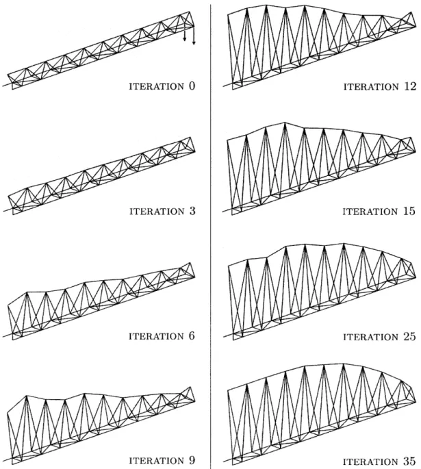
2.3.2

Planar Cantilever Truss Beam

A cantilever truss beam made of 10 segments is defined and parametrized as shown on figure 2.4. A truss segment is a group of members arranged in a pattern that is repeated in the direction of the beam. In this truss, each segment is made of 4 members: top, bottom, vertical and diagonal. The optimization variables are the lengths of the vertical members, and the objective is to minimize the end deflection.

hh

hi

hih

hn

4

L

Figure 2.4: Cantilever Truss Beam Parametrizetion

The following unitless values and constraints are imposed:

ho

=

10

L

=

105

1<hi

50 for i

= 1...10

A lower limit of 1 is used to prevent the truss from becoming unstable. The upper limit of 50 defines a reasonable search space for the optimization algorithm. No optimization variable reaches either limiting value, meaning that the search for the optimal geometry is not restricted by the constraints. The shape evolution leading to the optimal geometry (figure 2.5) is shown on the next page.

Figure 2.5: Cantilever Truss Beam Optimal Geometry

Considering the bending moment diagram, a triangular shape tapering towards the free extremity could have been expected. The oval shape obtained instead is due to the fixity. For the arbitrary combination of member sections and load magnitude considered in this example, the fixity is too short to allow for an optimized triangular shape. This phenomenon is shown on the three-dimensional cantilever truss-beam treated in section 2.3.5.

TRUSS GEOMETRY OPTIMIZATION

ITERATION

0. All optimization variables have an initial value of

so that each

truss segment is square. End deflection: 14.02

ITERATION

1. The depth of the beam starts growing at the fixity, creating a curved

shape. End deflection: 11.57

ITERATION

4. The increase in depth propagates towards the free extremity of the

beam. End deflection: 9.38

ITERATION 8.

Propagation stops approximately at mid-span. End deflection: 8.61

ITERATION

12. The shape is smoothed as the final adjustments of the optimization

variables are made. End deflection: 8.46

CHAPTER 2. TRUSS GEOMETRY OPTIMIZATION

2.3.3

Multi-Span Truss Bridge

Two similar truss bridges are optimized. Both bridges are made of 30 truss segments forming three spans and parametrized by the lengths of the vertical members. In the first bridge (figure 2.6), each span is an independent simply-supported truss beam. The second bridge (figure 2.7) is made of a single continuous truss beam resting on 4 supports. A uniform distributed load is applied at the bottom chord of both bridges. The objective is to minimize the aggregate deflection, defined as the sum of the maximum deflections of each span.

h

L1 L2 L3

Figure 2.6: Truss Bridge 1 Parametrization and Optimal Geometry

h 1 4 8 15 22 26 29

L L2 L3

Figure 2.7: Truss Bridge 2 Parametrization and Optimal Geometry

The following unitless values and constraints are imposed to both bridges:

L1 = 80 L2 = 140 L3 = 80 5 < hi < 25

In both cases, the optimal shape corresponds to the magnitude of the bending moment acting on the bridge. The optimal shape of the first bridge features a flat top chord at the middle of the longer span. At this location, where the bending moment is maximum, the optimization variables have reached the upper limit imposed by the constraints (h = 25), affecting the optimal shape expected. The shape evolution of both bridges is shown on the next page.

CHAPTER 2. TRUSS GEOMETRY OPTIMIZATION

Shape Evolution of Truss Bridge 1

Figure 2.8: Truss Bridge 1 Shape Evolution

Shape Evolution of Truss Bridge 2

-':7

CHAPTER 2. TRUSS GEOMETRY OPTIMIZATION

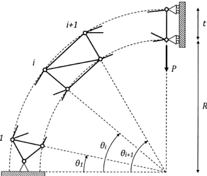
2.3.4

Semi-Circular Truss Arch

A semi-circular truss arch is modeled as a series of 20 truss segments, as shown

on figure 2.10. The arch is pinned at both fixities and a point load is applied at

mid-span.

Figure 2.10: Truss Arch Topology

In this example of truss geometry optimization, the overall shape of the structure

is fixed. The objective is to minimize the deflection at mid-span while keeping the

semi-circular appearance of the arch. It is known that semi-circular arches are not

the most efficient ones, so the design can only be partially optimized. This is a very

common situation in structural engineering, as architecture does not necessarily

compromise with structural efficiency.

The arch is set to remain semi-circular throughout the optimization process by

appropriately parametrizing the problem (see figure 2.11 p. 39). What is being

optimized is the distribution of the truss members within a semi-circular envelope.

Since the problem is symmetric, optimization is carried out on one half of the truss

arch only.