Categorical structural optimization : methods and applications

HAL Id: tel-02114558

https://tel.archives-ouvertes.fr/tel-02114558

HAL is a multi-disciplinary open access archive for the deposit and dissemination of sci-entific research documents, whether they are pub-lished or not. The documents may come from teaching and research institutions in France or abroad, or from public or private research centers.

L’archive ouverte pluridisciplinaire HAL, est destinée au dépôt et à la diffusion de documents scientifiques de niveau recherche, publiés ou non, émanant des établissements d’enseignement et de recherche français ou étrangers, des laboratoires publics ou privés.

Categorical structural optimization : methods and

applications

Huanhuan Gao

To cite this version:

Huanhuan Gao. Categorical structural optimization : methods and applications. Mechanics [physics.med-ph]. Université de Technologie de Compiègne; Université libre de Bruxelles (1970-..), 2019. English. �NNT : 2019COMP2471�. �tel-02114558�

Par Huanhuan GAO

Thèse présentée en cotutelle

pour l’obtention du grade

de Docteur de l’UTC

Categorical structural optimization: methods and

applications

Soutenue le 7 février 2019

Spécialité

:

Mécanique Numérique : Unité de recherche en

Mécanique - Laboratoire Roberval (FRE UTC - CNRS 2012)

U

NIVERSITÉ 

L

IBRE DE 

B

RUXELLES 

(ULB)

U

NIVERSITÉ DE 

T

ECHNOLOGIE DE 

C

OMPIÈGNE 

(UTC)

DOCTORAL THESIS 

Categorical Structural Optimization: 

Methods and Applications 

Author: 

Supervisor:

Huanhuan GAO 

Dr. Piotr B

Prof. Thierry M

Spécialité : Mécanique Numérique  

7 février 2019 

        ULB‐Building, Architecture, Town Planning and UTC‐Mécanique

iii

Declaration of Authorship

I, Huanhuan GAO, declare that this thesis titled, “Categorical Structural Optimiza-tion: Methods and Applications” and the work presented in it are my own. I confirm that:

• This work was done wholly or mainly while in candidature for a research de-gree at this University.

• Where any part of this thesis has previously been submitted for a degree or any other qualification at this University or any other institution, this has been clearly stated.

• Where I have consulted the published work of others, this is always clearly attributed.

• Where I have quoted from the work of others, the source is always given. With the exception of such quotations, this thesis is entirely my own work.

• I have acknowledged all main sources of help.

• Where the thesis is based on work done by myself jointly with others, I have made clear exactly what was done by others and what I have contributed my-self.

Signed: Date:

v

“As heaven maintains vigor through movements, a gentle man should constantly strive for self-perfection. As earth’s condition is receptive devotion, a gentle man should hold the outer world with broad mind. ”

vii

UNIVERSITÉ LIBRE DE BRUXELLES (ULB) UNIVERSITÉ DE TECHNOLOGIE DE COMPIÈGNE (UTC)

Abstract

ULB-École Polytechnique de Bruxelles and UTC-Génie Mécanique, Acoustique et Matériaux

ULB-Building, Architecture, Town Planning and UTC-Mécanique Doctor of Philosophy

Categorical Structural Optimization: Methods and Applications by Huanhuan GAO

The thesis concentrates on a methodological research on categorical structural op-timization by means of manifold learning. The main difficulty of handling the cat-egorical optimization problems lies in the description of the catcat-egorical variables: they are presented in a category and do not have any orders. Thus the treatment of the design space is a key issue. In this thesis, the non-ordinal categorical variables are treated as multi-dimensional discrete variables, thus the dimensionality of cor-responding design space becomes high. In order to reduce the dimensionality, the manifold learning techniques are introduced to find the intrinsic dimensionality and map the original design space to a reduced-order space.

The mechanisms of both linear and non-linear manifold learning techniques are firstly studied. Then numerical examples are tested to compare the performance of manifold learning techniques mentioned above. It is found that the PCA and MDS can only deal with linear or globally approximately linear cases. Isomap preserves the geodesic distances for non-linear manifold however, its time consuming is the most. LLE preserves the neighbour weights and can yield good results in a short time. KPCA works like a non-linear classifier and we proves why it cannot preserve distances or angles in some cases.

Based on the reduced-order representation obtained by Isomap, the graph-based evolutionary crossover and mutation operators are proposed to deal with categori-cal structural optimization problems, including the design of dome, six-story rigid frame and dame-like structures. The results show that the proposed graph-based evolutionary approach constructed on the reduced-order space performs more ef-ficiently than traditional methods including simplex approach or evolutionary ap-proach without reduced-order space.

In chapter 5, the LLE is applied to reduce the data dimensionality and a poly-nomial interpolation helps to construct the responding surface from lower dimen-sional representation to original data. Then the continuous search method of moving asymptotes is executed and yields a competitively good but inadmissible solution within only a few of iteration numbers. Then in the second stage, a discrete search strategy is proposed to find out better solutions based on a neighbour search. The ten-bar truss and dome structural design problems are tested to show the validity of the method. In the end, this method is compared to the Simulated Annealing algo-rithm and Covariance Matrix Adaptation Evolutionary Strategy, showing its better optimization efficiency.

In chapter 6, in order to deal with the case in which the categorical design instances are distributed on several manifolds, we propose a k-manifolds learning method based on the Weighted Principal Component Analysis. And the obtained manifolds are integrated in the lower dimensional design space. Then the method introduced in chapter 4 is applied to solve the ten-bar truss, the dome and the dame-like struc-tural design problems.

Keywords: Categorical Optimization, Structural Optimization, Manifold

Learn-ing, Dimensionality Reduction, K-manifolds LearnLearn-ing, Evolutionary Methods, Ker-nel Function, Polynomial Fitting, Truss Structure, Weighted Principal Component Analysis

ix

Acknowledgements

This research is supported by the China Scholarship Council (201406290021), the Na-tional Natural Science Foundation of China (No.11302173, No. 11620101002) and the Natural Science Foundation of Shaanxi Province (No. 2017JQ1037). I would like to express my sincere thanks to them.

I also want to thank my supervisor Prof. Rajan Filomeno Coelho. He has given so much care both on my research and my life. Even after he left ULB, he continued giving supervisions on my work. He is my first supervisor in Europe, I would never forget him.

I will give my gratitude to my supervisor Prof. Piotr Breitkopf. He has given me all kinds of help and supervision on my work, and has taught me a lot of research experience. Without him, I cannot finish my PhD career. Really thank you, Prof. Piotr Breitkopf.

I will also express my thanks to Prof. Thierry Massart has been in charge of all my administrative affairs in ULB since Prof. left ULB. He helped me with every regis-tration in ULB and organized the yearly defenses and the final PhD defense for me. Thank you so much, Prof. Thierry Massart!

I also want to thank Prof. Manyu Xiao. Even though she worked in China, she also gave me a lot of help and advise on my scientific research. Wish her a fruitful re-search life.

I will also thank my father and two sisters. It is them who gave me the courage to complete my PhD career. Ten thousand miles far away, I cannot stop my missing them.

My dear friends, Dong Yang, Yingli Chen, Zhe Chen, Weide Huang, Liang Meng, Anna Madra, Jinhua Xiao, Shanggui Cai, Jing Wen, Congcong Ma and so on, gave me a lot of help with my study and my life. They also brought me plenty of happi-ness and delights. With them , I feel that friendship is everywhere.

xi

Contents

Declaration of Authorship iii

Acknowledgements ix 1 Thesis overview 1 1.1 Research objectives . . . 1 1.2 Methodology . . . 1 1.3 Thesis outline . . . 2 2 Research background 5 2.1 Categorical structural optimization . . . 5

2.2 Machine learning and manifold learning. . . 8

2.3 Optimization methods . . . 10

2.3.1 Metaheuristics . . . 10

2.3.2 Gradient-based methods. . . 11

3 Manifold learning techniques 15 3.1 Principal component analysis . . . 16

3.2 Multidimensional scaling . . . 17

3.3 Isomap . . . 18

3.4 Locally linear embedding . . . 18

3.5 Kernel principal component analysis . . . 19

3.6 Testing examples . . . 20

3.6.1 Multiple cross-section example . . . 21

3.6.2 Swiss Roll example . . . 22

3.6.3 S-Curve example . . . 24

3.6.4 Time cost comparison . . . 26

3.6.5 Discussion on KPCA . . . 27

Data distance . . . 32

Angle change . . . 34

Conclusions on KPCA . . . 36

4 Categorical optimization: a discrete evolutionary approach 37 4.1 Background . . . 37

4.2 Representation of categorical variables . . . 38

4.3 Redundant dimensionality reduction. . . 39

4.3.1 Dimensionality reduction . . . 41

4.3.2 Multi-dimensional scaling . . . 41

4.3.3 Isomap . . . 42

4.3.4 Intrinsic dimensionality estimation. . . 43

4.4 Graph-based crossover and mutation operators. . . 44

4.4.1 Graph-based crossover operator . . . 44

4.5 Numerical tests . . . 46

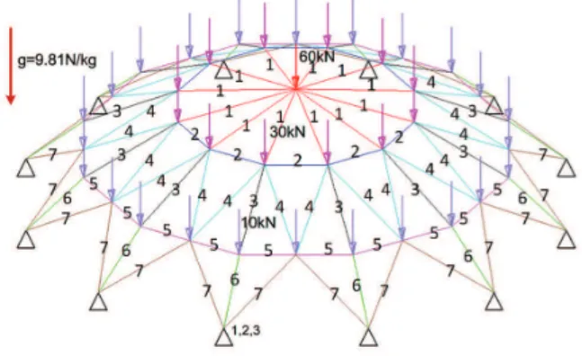
4.5.1 The dome structure optimization with single categorical variable 46 4.5.2 The dome structure optimization with seven categorical vari-ables . . . 47

4.5.3 Dam structure design . . . 50

4.5.4 Six-story rigid frame structure design . . . 53

4.6 Conclusions and prospects. . . 56

5 Categorical optimization: a two-stage search strategy 61 5.1 Background . . . 61

5.2 Categorical optimization statement . . . 62

5.3 Continuous search stage . . . 62

5.3.1 Dimensionality reduction . . . 63

5.3.2 The polynomial fitting and the fitting error estimation . . . 63

5.3.3 A practical fitting example and comparison. . . 65

5.3.4 The continuous search on the manifold . . . 70

5.4 Neighbour search stage. . . 71

5.4.1 Rounding-off criteria . . . 71

5.4.2 Neighbour search . . . 71

5.5 Numerical tests . . . 74

5.5.1 The ten-bar structure optimization problem. . . 74

5.5.2 The dome structure design problem . . . 83

5.5.3 Effects of neighbour search parameters . . . 84

5.5.4 Comparison of results . . . 89

5.6 A fast neighbour search algorithm . . . 93

5.7 Conclusions and prospects. . . 96

6 Categorical optimization: a k-manifolds learning approach 101 6.1 Background . . . 101

6.2 K-manifolds learning . . . 102

6.2.1 Weighted principal component analysis . . . 102

6.2.2 Optimization criteria . . . 103

6.2.3 Optimization problem statement . . . 104

6.2.4 Optimization algorithm for k-manifold learning . . . 105

6.2.5 A numerical test . . . 105

6.3 Numerical tests . . . 109

6.3.1 The 10-bar structure . . . 109

6.3.2 The dam structure . . . 110

6.3.3 The dome structure design . . . 112

6.4 Conclusions and prospects. . . 115

7 Conclusions, perspectives 119 7.1 Conclusions . . . 119

7.2 Perspectives . . . 120

A Questions frequently asked 121

B Attribute catalog of bars 123

C Attribute catalog of beams 127

xiii

List of Figures

2.1 The loads and responses of simulation . . . 6

2.2 Classifications of optimization by the nature of design variables . . . . 6

2.3 . . . 7

2.4 Methods of Metaheuristics and corresponding publication years . . . . 10

2.5 Gradient-based methods and the publication years. . . 13

3.1 Examples of non-linear manifolds . . . 16

3.2 Illustration of the geodesic distance. . . 18

3.3 The three types of cross-sections . . . 21

3.4 Cross-section instances . . . 22

3.5 The learning results obtained by different methods and parameters (Cross-sections) . . . 23

3.6 Sample points of the Swiss Roll . . . 24

3.7 The learning results obtained by different methods and parameters (Swiss Roll) . . . 25

3.8 Sample points of the S-Curve . . . 26

3.9 The learning results obtained by different methods and parameters (S-Curve) with 1000 sample points . . . 28

3.10 The learning results obtained by different methods and parameters (S-Curve) with 2000 sample points . . . 29

3.11 The learning results obtained by different methods and parameters (S-Curve) with 3000 sample points . . . 30

3.12 The learning results obtained by different methods and parameters (S-Curve) with 4000 sample points . . . 31

3.13 The values of z versus x21_{and x}11_{or x}22_{and x}12 _{. . . 33}

3.14 The values of z versus x21_{and x}11_{or x}22_{and x}12 _{. . . 34}

3.15 The relationship between θ0and θ1 . . . 36

4.1 Classification of design variables . . . 39

4.2 Instance representation in 3D space. . . 40

4.3 Illustration of 3-parameter continuous design space . . . 40

4.4 Illustration of using one parameter to describe a series of cross-sections 41 4.5 The flowchart of dimensionality reduction . . . 41

4.6 Illustration of the geodesic distance. . . 43

4.7 An example of dimensionality reduction of Fig. 4.2 using Isomap . . . 43

4.8 The graph-based crossover operator . . . 44

4.9 The graph-based mutation operator . . . 45

4.10 The dome structure with one categorical variable. . . 47

4.11 The mapping from 3D design space to 2D reduced-order space. . . 47

4.12 The design updating of Pareto sets in reduced-order space . . . 48

4.13 The improving performance of Pareto sets in objective space . . . 49

4.15 The evolutionary design history in objective space and the final Pareto

set . . . 51

4.16 The result comparison between the discrete manifold-learning approach and the rounded-off solution . . . 51

4.17 Designs comparison in design space: the better design (var1-7(G)) by the discrete manifold-learning approach and the rounded-off process from SQP solution (var1-7(SQP)) to nearest admissible instances . . . . 51

4.18 The dame-like structure . . . 52

4.19 The evolutionary design history in objective space and the final Pareto set . . . 52

4.20 The 6-storey rigid frame structure. . . 54

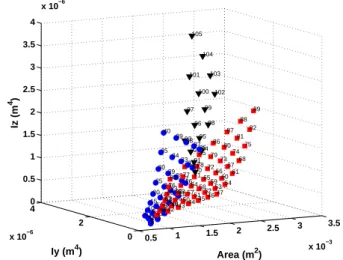
4.21 Design instances represented in reduced-order 3D space . . . 54

4.22 The evolution of designs in objective space and the final Pareto set . . 55

4.23 The result comparison between the discrete manifold-learning approach and the continuous solutions rounded off to the nearest admissible ones 55 4.24 The Pareto sets of selected generations obtained by the discrete mani-fold learning approach (DML) and simplex (S) of 20 different runs. . . 57

4.25 The fitting curve together with fitting error estimation of the Pareto sets obtained by both approaches . . . 58

4.26 The comparison of standard deviations estimation of the fitting errors 59 5.1 The three types of cross-sections . . . 65

5.2 The physical properties of 87 cross-sections . . . 66

5.3 The normalized physical properties . . . 66

5.4 The reduced-order 2D design space obtained by different manifold learning methods . . . 67

5.5 The comparison between the original and new 3D representation with different manifold learning methods . . . 68

5.6 The fitting errors for all the instances obtained by different manifold learning methods . . . 69

5.7 The mean errors of different manifold learning methods . . . 70

5.8 The maximum errors of different manifold learning methods . . . 70

5.9 Neighbour search for a single variable with two attributes . . . 73

5.10 The ten-bar structure . . . 75

5.11 The design history of the objective and constraints . . . 76

5.12 The evolution history of four variables in 2D space. . . 77

5.13 The evolution history of four variables in the original 3D space . . . . 78

5.14 The design history of the objective and constaints . . . 79

5.15 The evolution history of four variables in 2D space. . . 80

5.16 The evolution history of four variables in the original 3D space . . . . 81

5.17 The ten-bar truss design: the design history of the objective and con-straints . . . 82

5.18 The ten-bar truss design: the evolution history of four variables in 2D space . . . 82

5.19 The ten-bar truss design: the evolution history of four variables in the original 3D space . . . 83

5.20 The dome structure . . . 84

5.21 The dome structure design: the design history of the objective and constraints . . . 85

5.22 The dome structure design: the evolution history of four variables in 2D space . . . 86

xv

5.23 The dome structure design: the evolution history of four variables in

the original 3D space . . . 87

5.24 The design history of the objective and constraints . . . 95

5.25 The evolution history of four variables in 2D space. . . 97

5.26 The evolution history of four variables in the original 3D space . . . . 98

6.1 The three types of cross-sections . . . 105

6.2 The physical properties of 105 cross-sections . . . 107

6.3 The normalized physical properties . . . 107

6.4 The objective: total errors in each iteration. . . 108

6.5 The final three manifolds. . . 108

6.6 The integrated reduced representations of three manifolds . . . 109

6.7 The ten-bar structure . . . 110

6.8 The design history of the objective and constraints . . . 111

6.9 The evolution history of four variables in 2D space. . . 111

6.10 The evolution history of four variables in the original 3D space . . . . 112

6.11 The dam structure. . . 113

6.12 The design history of the objective and constraints . . . 113

6.13 The evolution history of 3 variables in 2D space . . . 114

6.14 The evolution history of 3 variables in the original 3D space . . . 114

6.15 The dome structure . . . 115

6.16 The design history of the objective and constraints . . . 116

6.17 The evolution history of 7 variables in 2D space . . . 117

xvii

List of Tables

3.1 The available values of geometrical parameters . . . 21

3.2 The corresponding learning time cost needed (Unit: s). . . 26

4.1 A catalog of bars’ physical features . . . 39

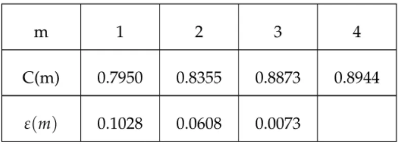
4.2 Correlation coefficients and ε versus dimension m . . . 46

4.3 Correlation coefficients and ε versus dimension m . . . 53

5.1 The available values of geometrical parameters . . . 65

5.2 The influence of search parameters . . . 88

5.3 The corresponding numbers of function evaluations . . . 88

5.4 Final feasible designs . . . 88

5.5 Optimization results by CMA-ES (1318 evaluations) . . . 89

5.6 Optimization results by CMA-ES (2652 evaluations) . . . 90

5.7 Optimization results by CMA-ES (2737 evaluations) . . . 90

5.8 Optimization results by CMA-ES (3182 evaluations) . . . 90

5.9 Optimization results by SA (1318 evaluations) . . . 91

5.10 Optimization results by SA (2652 evaluations) . . . 91

5.11 Optimization results by SA (2737 evaluations) . . . 92

5.12 Optimization results by SA (3182 evaluations) . . . 92

5.13 Objective comparison obtained by three methods . . . 92

5.14 Optimization objectives by neighbour search (NS) and the fast neigh-bour search (FNS) . . . 95

5.15 Evaluation numbers with neighbour search (NS) and the fast neigh-bour search (FNS) . . . 96

5.16 Optimization objectives by neighbour search (NS) and the fast neigh-bour search (FNS) . . . 96

5.17 Evaluation numbers with neighbour search (NS) and the fast neigh-bour search (FNS) . . . 96

6.1 The available values of geometrical parameters . . . 105

1 The attribute catalog of bar cross-sections for test 1 and test 2 in chap-ter 4 . . . 123

xix

List of Abbreviations

CSO Categorical Structural Optimization DR Dimensionality Reduction

PCA Principal Component Analysis

KPCA Kernel Principal Component Analysis WPCA Weighted Principal Component Analysis MDS Multi-Dimensional Scaling

LLE Locally Linear Embedding RBF Radial Basis Function GA Genetic Algorithms

EP Evolutionary Programming ES Evolution Strategy

CMAES Covariance Matrix Adaption Evolution Strategy SA Simulated Annealing

PSO Particle Swarm Optimization ACO Ant Colony Optimization SD Steepest Descend

MMA Method of Moving Asymptotes

GMMA Generalized Method of Moving Asymptotes

GCMMA Globally Convergent Method of Moving Asymptotes MFD Method of Feasible Directions

SLP Sequential Linear Programming SQP Sequential Quadratic Programming GRG Generalized Reduced Gradient

xxi

List of Symbols

X Coordinate matrix

Y Coordinate matrix after dimensionality reduction xj _{Coordinate of the j-th data point}

yj _{Reduced ordered Coordinate of the j-th data point} k_bj

The k-th element of the coordinate of the j-th data point n Number of data points

M Initial dimension of data points m Reduced dimension of data points C Covariance matrix

Φ Eigenvector metric

Λ Eigenvalue diagonal matrix Ψ Kernel function matrix ζ Kernel function

I Identity matrix wj The j-th weight

λi The i-th eigenvalue

φi The i-th eigenvector

ν Poisson’s ratio p Polynomial order

σ Parameter of Gaussian function K Stiffness matrix

u Displacement vector P Load vector

F Internal force of a bar

Fcr Critical load for linear local buckling

J Design objective function g Design constraint functions θ Angle variables

P Path on the manifold

H Height m L Length m t Thickness m r Radius m E Young’s Modulus N/m2 G Shear Modulus N/m2 ρ Density kg/m3

xxiii

1

Chapter 1

Thesis overview

In this chapter, an overview of the thesis is presented. In the first section, the objec-tives of the research are pointed out. Then we elaborate the general methodology of proposed optimization methods. In the last section, we give the outlines of the whole thesis.

1.1

Research objectives

The research objectives of the thesis are to improve the structural performances by using categorical optimization methods. More detailed objectives are listed as fol-lows:

• to study the working mechanism of manifold learning methods and to com-pare their performance with numerical tests.

• to refine the nature of design variables of categorical optimization and to state the categorical structural optimization problems.

• to develop a discrete graph-based evolutionary approach and a continuous-discrete two stage strategy to deal with the structural optimization problems. • to investigate how optimization algorithm parameters affect the optimization

results and optimization efficiency.

• to compare the performance of the proposed methods with that of current ma-ture optimization methods.

• to develop k-manifolds learning method to handle complex situations of the design space.

• to apply the proposed categorical optimization methods to truss structures composed with beams or bars.

1.2

Methodology

All the simulation processes in the thesis are carried out by using the finite ele-ment analysis packages of matlab software, including mass calculation, compliance evaluation and local linear buckling analysis. At first, the dimensionality of design space is reduced by certain manifold learning methods, then different methods are developed based on the reduced-order representations, including the graph-based evolutionary operators, the continuous-discrete two stage approach. In chapter 6, the design space of the optimization problems are firstly divided into several mani-folds, and then dimensionality reduction is applied to each manifold. The proposed

optimization methods are tested on practical numerical structure design problems, showing their validity and optimization efficiency.

1.3

Thesis outline

In chapter 1, the thesis overview is given. The main goals of the research include the investigation of manifold learning methods, the statement of categorical opti-mization problems, the development and application of optiopti-mization methods and the evaluation of the proposed optimization methods. In the methodology part, the dimensionality of the design space is reduced by manifold learning methods, in-cluding the k-manifolds learning method. Then the discrete evolutionary approach and the two-stage search approach based on the reduced order representations are applied to structure design problems. The three principal parts, including manifold learning, simulation and optimization, are carried out with matlab packages. In the outline part, the general introduction of the whole thesis is presented.

In chapter 2, the research backgrounds and references are listed. Since the research content of the thesis is a combination of structural optimization and categorical op-timization, both of them are detailed introduced, with different kinds of design cri-teria and optimization classification. In the second section, the related concepts of machine learning, together with their corresponding working mechanisms, are ex-plained based on previous scientific works. Among all the machine learning meth-ods, manifold learning are specially emphasized since it plays a key role in our methodology. The typical manifold learners, including both linear and non-linear ones, are elaborated with the aide of corresponding publications. The final section discusses the optimization methods which consist of metaheuristics and gradient-based methods, together with comments on their performance.

Chapter 3 mainly introduces the mechanisms of several manifold learning tech-niques, including principal component analysis (PCA), multi-dimensional scaling (MDS), Isomap, locally linear embedding (LLE) and kernel principal component analysis (KPCA). Then three testing examples are used to compare the manifold learning results. Besides, the learning efficiency is also discussed. As a focusing point, KPCA is specially discussed on its failure to length and angle preservation. Chapter 4 presents a discrete evolutionary graph-based approach to handle categor-ical optimization problems. This approach deals with multi-objective optimization with a single manifold design space. The higher dimensional design space is firstly mapped to lower dimensional pace by applying the non-linear leaner Isomap, then the design instances are connected using k-means or r-means. The evolutionary op-timization operators including crossover and mutation are developed based on the lower dimensional connecting graph. Finally, the algorithm is tested by numerical examples including the dome and dam structure and six-story rigid frame structure. The optimization results and efficiency are compared with a continuous method and simplex approach, showing the advantages of the proposed algorithm.

In chapter 5, a two-stage search approach is proposed to handle single-objective optimization problems with a single manifold design space. In the first stage, the original design space is mapped to a lower dimensional space by LLE, then we con-struct the analytical mapping from lower dimensional space to original one. Thus the design problem is transformed to a lower order one. We make the discrete prob-lem continuous and utilize the gradient-based method to execute a rough search. In the second stage, a neighbour search based on the connecting graph is developed and applied to numerical examples. The proposed approach is also compared with

1.3. Thesis outline 3 metaheuristics. In order to improve the optimization efficiency, a gradient-based fast neighbour search is proposed for the second search stage.

Chapter 6 proposes a k-manifolds learning methods aiming at finding multiple man-ifolds in the observation space and its application to single-objective categorical structural optimization problems. Before dimensionality reduction, each design in-stance is attached with a weight which donates the contribution in the process of PCA. By optimizing the weights, the k-manifolds are separated automatically. Then the lower dimensional representations of k-manifolds are organized and merged in the same space. The categorical structural optimization is executed based on the lower dimensional space of k-manifolds. Numerical examples are also tested in or-der to show the validity of the methods.

Chapter 7 presents the conclusions and perspectives of the whole thesis. The con-clusions include the evaluations of different kinds of manifold learning methods, the effectiveness and optimization efficiency of three categorical optimization methods: the discrete evolutionary approach, the two-stage search methods and k-manifolds learning based approach. The further development and perspectives of the pro-posed methods are also given in this chapter.

5

Chapter 2

Research background

2.1

Categorical structural optimization

As a powerful design and selection tool, optimization is widely used or embed-ded in both research subjects and engineering design applications due to its strong mathematical background, flexible interfaces, various forms and design automation property, for example, the identification and characterization problems (also named the inverse problems) (Mosselman, Polman, and Dijkema,1996), machine learning subjects (Tenenbaum, De Silva, and Langford,2000), route planning (Fu, Ding, and Zhou,2012), structural optimization (Cheng and Guo,1997; Bendsøe,1989) et al. Among all the applications of optimization techniques, structural optimization is "a discipline dealing with optimal design of load-carrying mechanical structures" (by Krister Svanberg). The general framework of structural optimization includes an op-timizer part and a simulation part (or response estimation). The role of the opop-timizer is to update the designs iteration by iteration according to performance of the struc-ture. In gradient-based optimizer, the sensitivities of all the criteria with respect to each design variables are requested to renew the designs. While in population-based evolutionary optimizers, the sensitivities are not necessary, and the population is up-dated in successive generations.

The main task of the simulation (Fig. 2.1) part is to calculate the responses of the structure, including weight (mass) or volume (Kaufmann, Zenkert, and Wennhage,

2010), structural compliance (or strain energy) (Sigmund, 2001), maximum stress (Duysinx and Bendsøe, 1998), natural vibration frequency (Kaveh and Zolghadr,

2011), dynamic responses (Biegler, 1984), local or global buckling (Lund, 2009) et al. The loads which are applied to the structure contain static loads (Sigmund,2001), acceleration loads (including gravity) (Xie and Steven,1997), time-variant dynamic incentives (Branke et al.,2000), thermal loads (Li et al.,1999), electromagnetic loads (Chun et al.,1997) et al.

From the formal point of view, optimization may be classified by different kinds of features. According the number of objectives, we can divide optimization problems into single objective optimization (Liang et al.,2014) and multi-objective optimiza-tion (Deb et al.,2002). Furthermore, considering the number of design constraints, we can classify optimization into constrained problems (Powell,1978) and uncon-strained problems (Dennis Jr and Schnabel,1996). One can also classify optimiza-tion types by methods used, for example, the gradient-based optimizaoptimiza-tion (Snyman,

2005), the evolutionary optimization (Davis,1991), memetic optimization (Moscato,

1989) et al.

The so-called categorical optimization is labelled from the optimization classifica-tion based on the nature of design variables. In the principal level, we can divide optimization problems (Fig. 2.2) into continuous optimization, non-continuous op-timization and mixed-variable opop-timization. Among them, continuous opop-timization

FIGURE2.1: The loads and responses of simulation

FIGURE2.2: Classifications of optimization by the nature of design

variables

denotes the optimization problems in which the design variables are all continuous (Pan et al., 2010; Zhao et al., 2011). While non-continuous optimization includes discrete optimization, categorical optimization. The discrete optimization (Deo and Kowalik,1983; Rajeev and Krishnamoorthy,1992) indicates that the design variables are all discrete (or integer), which means the corresponding design space collapses into a set of discrete points. We need to note that, in discrete optimization, the design variable can only take scalar values, despite of that it may be handled with binary strings or other means. Different from the discrete one, categorical optimization (Coelho et al., 2015; Sloane and Morgan, 1996) can be defined as the optimization where design variables (we say categorical variables) can take the values of a finite set of instances, which were regarded as non-numerical ones in the beginning. While in our work, we represent those instances with vectorial data, which can clearly re-veal the nature of categorical variables: they are multi-dimensional discrete vari-ables. And this point will be elaborated in more detail.

From the viewpoint of problem types, structural optimization can be subdivided into topology (Sigmund,2001), shape (Rozvany, Zhou, and Birker, 1992), size (La-porta and Brussard, 1991), material selection (Stegmann and Lund, 2005), cross-section selection et al (Fig. 2.3). Among these categories, the topology optimiza-tion (Fig. 2.3(a)) deals with the layout design of materials or parts under given set of loads and boundary conditions, for example the topology optimization of con-tinuum structure (Duysinx and Bendsøe,1998) and the truss topology optimization (Rozvany, 1996). The former is usually treated with continuous variables, mean-while the latter is always handled in a discrete manner. The shape optimization (Fig. 2.3(b)) optimizes the boundary of a part, for example the radius of structural

2.1. Categorical structural optimization 7

(a) Topology optimization (b) Shape optimization

(c) Size optimization (d) Material selection

FIGURE2.3

holes (Lee and Kim,2010a). The widely used shape optimization techniques include geometrical parameter control (Hilbert et al.,2006), Isogeometry (Wall, Frenzel, and Cyron, 2008), level-set functions (Allaire, Jouve, and Toader, 2002), control points (Nemec, Zingg, and Pulliam,2004) et al. Size optimization (Fig. 2.3(c)) (Kaveh and Talatahari,2009) focuses on the geometrical parameters of a structural feature, for ex-ample the length of a bar, the thickness of a shell. The material selection (Fig.2.3(d)) aims at finding the best material combinations for different parts of the structure (Zhou, Yin, and Hu,2009; Ashby,2000). To handle the material selection problems, both continuous methods and discrete methods can be applied.

The categorical structural optimization is the combination of categorical optimiza-tion and structural optimizaoptimiza-tion, for instance, the selecoptimiza-tion of a material within a fi-nite the set (steel, aluminium, titanium, composites) or the selection of cross-section types among the catalog (square, I-shaped, round,...). The key issue with this kind of problems is how to represent the design variables (Coelho et al.,2015; Filomeno Coelho,2014).In previous work, different coding schemes including binary, real and simplex, are proposed successively. Binary coding (Goldberg, 2006) can only rep-resent non-continuous values with 0/1 strings which may lead to the problems of expression accuracy, excess non-sense strings et al. Real coding utilizes the real val-ues to stand for representation and optimization, thus the genotype and phenotype are united into one (Herrera, Lozano, and Verdegay, 1998; Eshelman and Schaffer,

1993). But when dealing the categorical variables, both binary coding and real cod-ing will casually assign unfounded distances (or called relative positions) to cat-egorical data. To overcome the distance expression difficulty, the simplex coding (Filomeno Coelho,2014; Herrera et al., 2014) is proposed and applied in categori-cal optimization. Instead of using binary strings or real numbers, simplex coding exploits vectorial coordinates of points in the design space, in which different cat-egorical design candidates are assigned as the same. The other optimization meth-ods which are tailored for categorical optimization include the mesh adaptive direct

search (Abramson et al.,2009), ant colony (Liao et al.,2014), mixed variable program-ming (Kokkolaras, Audet, and Dennis,2001) and global descent approach (Lindroth and Patriksson,2011).

2.2

Machine learning and manifold learning

The objective of manifold learning (Lunga et al.,2014; Tenenbaum, 1998) is to find the potential lower dimensional topological space embedded in the higher dimen-sional space. The original higher dimendimen-sional space is named observation space while the lower dimensional space is called feature space. Manifold learning is a kind of unsupervised machine learning method. The various machine learning theories and methods can be generally divided into three learning method groups: distinction construction and classification, conditional probability construction and probability density function construction through regenerative models.

The distinction construction and classification methods include clustering analysis, pattern recognition, artificial neural networks, support vector machines, manifold learning, Bayesian classifier and decision tree.

Among those learning methods, clustering analysis (Hartigan,1975; Jain and Dubes,

1988; Hartigan and Wong,1979) groups a certain number of sample points in differ-ent clusters based on the distance definition (for example the Euclidean distance) or on the similarity according to data features, and it has been applied in economics, computer science and web techniques.Pattern recognition (Nasrabadi,2007; Anzai,

2012) concentrates on finding of data regularities and patterns, and assigns differ-ent labels to input values according to the learning results. Inspired by the bio-logical neural networks, artificial neural networks (Schalkoff,1997; Yegnanarayana,

2009) exploit the multi-layer neuron which work as simple linear or non-linear clas-sifiers to distinguish different kinds of categories through a big amount of learning examples. The artificial neural networks also have a wide application in artificial intelligence, vehicle control, face identification, signal classification. They are also referred as a king of deep learning. Support vector machines (Suykens and Van-dewalle,1999; Furey et al.,2000) are a kind of supervised learning methods which can analyse the training data and build up learning models for classification and regression analysis. Manifold learning (Lunga et al.,2014; Tenenbaum,1998) aims to find the lower dimensional representation of higher dimensional data with no (or less) information loss. It is also regarded as a kind of dimensionality reduction technique. It is used in image management, structural optimization. We will give a detailed introduction to manifold learning later in chapter 2. The Bayesian classifiers (Wang et al.,2007; Domingos and Pazzani,1997) are sets of probabilistic classifiers taking advantages of the Bayes’ theorem by assuming that the features are strongly independent (naive Bayes). Bayesian classifiers have achieve a great success in text check, speech recognition and human-level concept learning (Lake, Salakhutdinov, and Tenenbaum,2015). The decision tree (Quinlan,1986; Quinlan,1987) applied the tree model with decisions and their possible consequences in order to make deci-sions. It is simple and well interpreted, but it may also bring inaccuracy in result outputs , thus cause wrong decisions.

The second group of machine learning methods: conditional probability construc-tion, mainly contain the Gaussian process regression, linear discriminant analysis, nearest neighbor methods, radial basis function kernels (Chang et al., 2010; Vert, Tsuda, and Schölkopf,2004). In Gaussian process regression, the lazy learning and

2.2. Machine learning and manifold learning 9 the kernel function are used to predict the value of given training data, providing both of the value estimation and the uncertainty information. The Gaussian process learning can be a helpful tool to predict and build up the surrogate model of a func-tion, for example the kriging model. Linear discriminant analysis (Mika et al.,1999; Altman, Marco, and Varetto,1994; Prince and Elder,2007) applies a linear combina-tion of features to classify or separate different kinds of events, and it is commonly used in pattern recognition, statistics and machine learning. The nearest neighbor methods (Shakhnarovich, Darrell, and Indyk,2006; Devroye and Wagner,1982) can be regarded as a kind of lazy learning. In the nearest neighbor methods, the investi-gated function is approximated locally, then the object is classified only by a majority vote of its neighbors. Due to its simplicity, the nearest neighbor methods are widely used in classification and regression fields. The radial basis function kernels (Chang et al.,2010; Vert, Tsuda, and Schölkopf,2004) are also named Gaussian RBF. They are popular in all the kernel-related learning methods, for example the support vector machine and the kernel principal component analysis. And in chapter 2, we give an exhaustive elaboration of the radial basis function.

The third learning algorithm group is the probability density function construction through regenerative models. They can be divided to expectation-maximization al-gorithm, probability models and generative topographic mapping. Among them, the expectation-maximization algorithm (Zhang, Brady, and Smith, 2001; Moon,

1996; Fessler and Hero,1994) deals with the statistical models which are dependent on unobserved latent variables. The method can find the maximum likelihood esti-mates of the parameters in an iterative manner. The probability models (Barlow and Proschan,1975; Ross,2014) can build the relationship between several independent random variables by using the graph theory. The graphs used in probability models include the Bayesian networks and the Markov networks. This method is usually used in Bayesian learning and machine learning. The generative topographic map-ping (Bishop, Svensén, and Williams,1998) projects a low dimensional data to a high dimensional space by a smooth function considering noise, then the expectation-maximization algorithm is used to learn the parameters of the low dimensional dis-tribution and the noise. The advantage of this method is that the shrinking neigh-bourhoods or decreasing step lengths are not necessary for algorithm convergence. There are two kinds of linear manifold learning methods which are named Princi-pal Component Analysis (PCA) (Jolliffe, 1986; Wold, Esbensen, and Geladi, 1987) and Multi-Dimensional Scaling (MDS) (Martin and Eroglu,1993; Kandogan,2001), respectively. PCA investigates the covariance matrix of the observed data and de-composes it through eigenvalue decomposition. Consequently, PCA reorganizes the projection system by minimizing the variance, thus it can preserve the most of the information. MDS acts on the inter-distances between data points. It focuses on the preservation of Euclidean distances. Normally, the results obtained by PCA and MDS are the same, but PCA provides an explicit expression which can map new ex-tra points while MDS cannot handle that. The main disadvantage of PCA and MDS is that they are not able to handle non-linear data, for example the "Swiss Roll" man-ifold (Tenenbaum, De Silva, and Langford,2000).

The well-known non-linear manifold learning methods include Locally linear Em-bedding (LLE), Isomap and Kernel Principal Component Analysis (KPCA). LLE (Roweis and Saul,2000; De Ridder et al.,2003; Donoho and Grimes,2003) consists of three steps: Firstly, LLE builds the neighbourhood for each sample point by using either k-neighbour means or r-radius means; Secondly, LLE constructs the weights of all neighbours by minimizing the construction error. One of the advantages is that the weight optimization problem is convex and thus local minima can be avoided.

FIGURE2.4: Methods of Metaheuristics and corresponding publica-tion years

Isomap (Tenenbaum, De Silva, and Langford,2000; Balasubramanian and Schwartz,

2002) can be regarded as a non-linear version of MDS. What is different between MDS and Isomap is that Isomap applies the geodesic distances instead of Euclidean distances. In Isomap, the geodesic distance is calculated by the Dijkstra algorithm (Dijkstra,1959), then the distances are preserved in the lower dimensional design space. The dimensionality reduction effects of Isomap actually heavily depends on the construction of the neighbourhood connecting graph. If the graph cannot re-flect the true manifold in the higher dimensional space, the Isomap will fail. Also, Isomap has the same disadvantages as MDS, namely Isomap cannot deal with new data points and needs the target dimension number is given in advance. KPCA (Schölkopf, Smola, and Müller,1998; Cao et al.,2003) firstly maps the original data to much higher dimensional space by using the kernel functions, for example the linear kernel function, the polynomial kernel function and the Gaussian radial ba-sis function. Then PCA is utilized to reduce the dimensionality. This is the classi-cal idea of Support Vector Machines (Cortes and Vapnik,1995; Vapnik,2013). The dimensionality reduction effects of KPCA mainly depend on the choice of kernel functions and the parameters of the kernel functions. Those non-linear manifold learning techniques have already been used in identification problems (Meng et al.,

2015), structural optimization (Raghavan et al., 2013), visualization problems (Pat-wari, Hero III, and Pacholski,2005; Wang et al.,2008) and networks (Patwari and Hero,2004).

2.3

Optimization methods

2.3.1 Metaheuristics

The metaheuristics denote a process of generating and selecting good solutions within a limited acceptable time cost. Normally the global optima cannot be guaranteed or proved by metaheuristics. Despite of the cons, metaheuristics still have received more and more attentions and are applied to handle numerous engineering and re-search optimization problems.

The popular representative methods of metaheuristics (Fig. 2.4) include ant colony optimization (ACO), genetic algorithms (GA), evolution strategy (ES), evolution-ary programming (EP), simulated annealing (SA) and particle swarm optimization (PSO).

2.3. Optimization methods 11 Colorni,1996) was firstly used to find the optimal path based on the food-seeking behaviours of ants. Then it is extended and diversified to solve many kinds of opti-mization problems. It is a kind of simulated evolutionary algorithm. Nowadays, the ant colonies optimization is usually used in route planning, scheduling, resource al-location problems et al. The genetic algorithms (Davis,1991; Anderson-Cook,2005) are a kind of nature-inspired method to deal with optimization problems. They sim-ulate the evolution of biological populations and apply the "survival of the fittest" idea. The main operators of genetic algorithms consists of initialization, crossover, mutation and selection. Due to the flexibility of coding schemes, operator extensibil-ity and interface versatilextensibil-ity, genetic algorithms have achieved much success both in theoretical and engineering applications (Goldberg and Holland,1988; Srinivas and Deb,1994). In evolution strategy (Janis,1976), the design evolution is inspired only by mutation and selection in one generation. The evolution continues until the ter-mination conditions are satisfied. In order to generate new populations, the normal distribution is used to generate new random individuals. The mutation strength is controlled by self-adaptation schemes. If the individual step size is determined by covariance matrix, the corresponding algorithm is named covariance matrix adap-tation evolution strategy (CMA-ES) (Hansen, Müller, and Koumoutsakos,2003; Ros and Hansen,2008). evolutionary programming (Back,1996) has many similarities with genetic programming. In EP, the new variation is only driven by mutation op-erators which act on the population, then the survivor selection is applied to main-tain good individuals for next generation. The applications of EP include artificial intelligence (Fogel, Owens, and Walsh,1966; Fogel,1999), machine learning, struc-tural optimization. The simulated annealing (Kirkpatrick, Gelatt, and Vecchi,1983) is a probabilistic optimization method for finding the global optimum of the objec-tive over a large search space within a fixed time cost by simulating the process of metal annealing. The whole simulation process is controlled by the annealing tem-perature, which determines by how much probability the new design is accepted or rejected. By accepting and rejecting operation, the design has a certain possibility to walk out of the current local optima and find the global one. The particle swarm optimization (Kennedy,2011; Poli, Kennedy, and Blackwell, 2007) is also a famous population based optimization method. The method regards every individual as a micro particle without any volume and mass, and every particle moves in the de-sign domain with a certain speed according to the flying experiences of its own and its neighbours. All the particles are supposed to concentrate on better solutions. In further development, the inertia weights are introduced to control the exploitation and exploration properties. When orthogonal learning (Zhan et al.,2011; Ho et al.,

2008) is introduced into PSO, the global convergence, convergence accuracy and ro-bustness have been significantly improved.

Other metaheuristics optimization methods include artificial immune systems (AIS) (Aickelin, Dasgupta, and Gu,2014), cultural algorithms (CA) (Reynolds,1994), co-evolutionary algorithms (CEA) (Michalewicz and Nazhiyath,1995), differential evo-lution (DE) (Storn and Price,1997), genetic programming (GP) (Koza,1992), greedy adaptive search procedures (GASP) (Feo and Resende,1995).

2.3.2 Gradient-based methods

Different from metaheuristics, the gradient-based methods also represent a large group of iterative design updating methods taking the advantage of gradients (also called sensitivities) of the objective function and constraint functions with respect

to design variables. For multiple variable optimization problems, the first order sensitivities can be organized in the form of Jacobian vector, and the second order sensitivities are written in the form of Hessian matrix.

The basic gradient-based methods include the steepest descent (SD), conjugate gra-dient (CG), Newton’s method (NM), as shown in Fig. 2.5. The steepest descent (Goldstein,1965; Yamada,2001) is a classical first-order optimization method. It uti-lizes the reverse direction of the gradients as the searching direction, and finally one can expect that the searching process converges in a local solution. The advantages of steepest descent is that it is simple, but it suffers from the so called "sawtooth phenomenon" which leads to a slow convergence. Furthermore, the steepest de-scent method does not consider design constraints, so modifications are necessary, for example the penalty function methods (Kort and Bertsekas,1972). The conjugate gradient (Powell,1977) is also method to solve unconstrained optimization prob-lems. By applying the conjugate property of the adjacent searching directions in the optimization loops, the conjugate gradient introduces a modification of current searching direction, making it faster than the steepest descent in the beginning, but this modification may also be not conducive to the convergence speed due to error accumulation in final several iteration. The Newton’s method (Wedderburn, 1974; Loke and Barker,1996) (also named Newton-Raphson method) uses both of the first-order and second-first-order gradients (Hessian matrix) to construct a second-first-order ap-proximation of the objective function. Many analytical tests have proved that in the case where the Newton’s method is applicable, it is faster than the steepest descent. However, one of the difficulties for Newton’s method is that the Hessian matrix is usually hard to obtain. And an fatal condition required is that the Hessian matrix must be positive definite. In order to solve this problem, a series of quasi Newton’s methods (Shanno,1970) are proposed and developed, including the DFP algorithm (Broyden,1970) and BFGS algorithm (Zhu et al.,1997). The idea of both algorithms is to approximate the Hessian matrix in order to complete optimization search under the quasi Newton’s conditions.

The practical gradient-based optimization methods (Fig. 2.5) used for engineering problems include the method of feasible directions (MFD), sequential linear pro-gramming (SLP), sequential quadratic propro-gramming (SQP), generalized reduced gradient (GRG), method of moving asymptotes (MMA) et al. The method of fea-sible directions (Zoutendijk,1960; Chen and Kostreva,1999) can be regarded as an extension of unconstrained gradient descent. It starts at the initial design point, and applies the 1-D line search along the descent direction. The key step is the choice of search directions and searching step lengths. The method of feasible di-rections can solve the optimization problems with inequality constraints at a fast speed, however, it can not deal with the optimization problems with equality con-straints. Sequential linear programming (Marcotte and Dussault, 1989; Etman et al., 1996) is proposed to handle non-linear optimization problems by using first-order approximation. This method solves a sequence of first-first-order approximations of the original problem, which provides a high optimization efficiency. At last, the trust regions techniques are introduced to guarantee converged optimization cess. Similar as the sequential linear programming, the sequential quadratic pro-gramming (Nocedal and Wright,2006; Boggs and Tolle,1995) solves a sequence of sub-problems which are approximated by quadratic models with linear constraints. If the optimization problem is unconstrained, the sequential quadratic programming degenerates to Newton’s method; If only equality constraints exist, this method evolves to Newton’s method with Karush–Kuhn–Tucker conditions of the optimiza-tion problem. The generalized reduced gradient (Lasdon et al.,1978) is the general

2.3. Optimization methods 13

FIGURE2.5: Gradient-based methods and the publication years

form of the reduced gradient method (Wolfe,1962; Minyi and Jiye, 1979) to solve optimization problems together with non-linear objective function and non-linear constraints. In this method, the inequality constraints are firstly transformed into equality constraints by introducing a positive slack variable. Then the all the design variables are divided into independent and dependent variables according to the all the equality constraints, consequently the dependent variables are represented by the independent ones. After that, the size of the gradient information is reduced. Then the Newton’s method is applied to solve the non-linear equation sets and ob-tain a proper searching step length until the algorithm is converged. The method of moving asymptotes (Svanberg,1993; Svanberg,1987) uses the asymptotes iteration by iteration to control the constructed convex sub-problems being solved, which can help improve the convergence speed and optimization stability. The further devel-opments include the generalized method of moving asymptotes (Zhang et al.,1996) and the globally convergent method of moving asymptotes (Zillober,1993).

15

Chapter 3

Manifold learning techniques

In this chapter, we give an introduction of several popular manifold learning algo-rithms. The role of manifold learning is crucial because all the proposed optimiza-tion methods are developed based on the manifold learning techniques. All the manifold learning methods assume that the data points are randomly sampled from an m-dimensional manifold which exists potentially in an M-dimensional space (m<M). The task of manifold learning is to find the new representations (coordi-nates) of those sample points in the lower m-dimensional space, according to their coordinates in the higher M-dimensional space. Conventionally, the original higher dimensional space is called observation space, while the new lower dimensional space is named feature space.

The manifold learning algorithms are mainly categorized into two kinds: the linear and non-linear ones. There have already been theories and applications which con-centrate on the linear manifold learning, for example, a linear manifold indicates a 1-D line, 2-D plane, or a hyperplane in the higher dimensional observation space. Although in some cases, the potential manifold is assumed to be linear, it is gen-erally non-linear in most practical cases. Another fact is that since the data points are obtained by measurements or observations, it is unavoidable to introduce the observation error, or we say noise, which will undermine the original linearity of the data. Consequently the linear manifold is always used as a realistic assump-tion rather than an ideal tool. Even though, we cannot ignore the successful theory developments and numerous practical applications of linear manifold learning tech-niques because firstly non-linear manifold can always be regarded as locally linear and secondly, linear manifold learning techniques usually have high efficiency in dealing with non-linear data, especially for big data and large dimensionality num-bers.

The non-linear manifold learning takes more complex manifolds in consideration, for example, manifolds with bending, warping or twisting. The famous examples for scientific research purposes are the "Swiss Roll" and the "S-Curve", as shown in Fig.

3.4. Undoubtedly, non-linear manifolds are closer to the real data status of the world. The task of non-linear manifold learning is to recover the lower dimensional coordi-nates with provided higher dimensional representations of the non-linear data.

The well-known linear manifold learning algorithms include Principal Component Analysis (PCA) and Multidimensional Scaling (MDS) illustrated in section 3.1 and 3.2. Three typical non-linear manifold learning techniques are also introduced in this chapter, including Isomap (section 3.3), Locally Linear Embedding (LLE) (section 3.4) and Kernel Principal Component Analysis (KPCA) (section 3.5), respectively. In section 3.6, we give testing examples of the proposed manifold learning techniques.

−10 −5 0 5 10 15 0 10 20 30 −15 −10 −5 0 5 10 15 x y z

(a) Swiss roll

−1 −0.5 0 0.5 1 0 2 4 6 −1 −0.5 0 0.5 1 1.5 2 2.5 3 x y z (b) S-Curve

FIGURE3.1: Examples of non-linear manifolds

3.1

Principal component analysis

We firstly define the data X = [x1_{, x}2_{,· · · , x}n_{]is a M×n matrix. M is the number}

of dimensions, while n is the number of data points. Dimensionality reduction is to find a lower m-d representation of the n data points.

Suppose the initial data X is centered in the beginning, then the covariance matrix can be defined as:

C= 1

nXX

T

. (3.1)

The eigenvalue decomposition yields:

C=ΦΛΦT_{, (3.2)}

whereΛ denotes the eigenvalues and Φ is the metric of corresponding eigenvectors, andΦTΦ_{=I. Note that after a descending ordering}

Λ=diag(λ1, λ2,· · · , λM),

λ1 ≥λ2 ≥ · · · ≥λM.

(3.3) We choose the first m eigenvectors and form the projection matrixΦm= [φ1, φ2,· · · , φm].

Finally, we obtain the representation in m dimensional space: yi_=ΦT

mx i

, i=1, 2,· · · , n. (3.4)

With Eq.3.4, we can project new points to the lower dimensional space.

After dimensionality reduction, the data information preservation ratio of the lower dimensional representation can be measured by:

κ = m ∑ i=1 λi M ∑ i=1 λi . (3.5)

κ=1 means no information loss during the mapping process and the m is the num-ber of intrinsic dimensionality.

3.2. Multidimensional scaling 17

3.2

Multidimensional scaling

Multidimensional scaling is also a linear manifold learning algorithm. Different from PCA, MDS focuses on the distance preservation. Given the distance matrix:

D(nX×)n, D (X)₍ i, j) = ||(xi , xj_)|| 2, i, j=1, 2,· · · , n, (3.6)

where|| · ||2is the 2-norm of a vector, MDS is developed to find the new coordinates

Yin lower dimensional space:

Ym×n = [y1, y2,· · · , yn], yi _{= (}1_bi ,2_bi ,· · · ,m_bi₎T_{, i=1, 2,· · · , n,} n

∑

In order to handle centred data, the transformation matrix P is defined as: P=I− 1

nee

T

, eT _{= (}

1, 1, 1,· · · , 1)₁×n, (3.8)

yielding the Gram matrix G:

G= −1

2P(D

(X)₎2

PT

(3.9) Because G is symmetric and positive definite, we carry out the eigenvalue decom-position and get:

G= ΦΛΦT , (3.10) where Λ=diag(λ1, λ2,· · · , λM), λ1 ≥λ2 ≥ · · · ≥λM (3.11) andΦ is the matrix whose columns contain eigenvectors of G and λicorresponds to

the i-th largest eigenvalue.

We choose the m largest eigenvalues and define: Λ12 m = [diag( p λ1, p λ2,· · · , p λm)] (3.12)

Finally we obtain the reduced-order coordinate matrix Y: Y= [y1

, y2

,· · · , yn_{] =Λ}12

mΦT_m. (3.13)

whereΦmis composed by the eigenvectors corresponding to the m largest

eigenval-ues.

Different with PCA, MDS cannot add new points after the the process is completed. Another difference is that MDS needs the target dimensionality number given in advance, while PCA can decide the target dimensionality number after eigenvalue decomposition.

x

x

(a) Geodesic distance

The shortest path from xa to xb

x

x

(b) The shortest path

FIGURE3.2: Illustration of the geodesic distance

3.3

Isomap

As a non-linear manifold learning method, Isomap can be regarded as a variant of MDS. The difference between MDS and Isomap is that MDS uses the Euclidean distances while Isomap utilizes the geodesic distances. Geodesic is the line along which the acceleration vector equals zeros on the manifold. In Isomap, the geodesic distance is approximated by the shortest path based on graph algorithm.

Fig. 3.2(a) shows the illustration of a geodesic from point xa _{to x}b_{. In order to}

cal-culate the geodesic distance, we first define the nearest neighbour points for all the points by the ε-mean or the K-mean algorithm(Tenenbaum, De Silva, and Langford,

2000). Then, for every pair of neighbour points, their geodesic distance is approx-imated by the Euclidean distance; for other nonadjacent points, their geodesic dis-tance is approximated by summing up the disdis-tances along the shortest path obtained by Dijkstra algorithm (Dijkstra,1959) in the graph (Fig. 3.2(b)).

After obtaining the distance matrix, the MDS algorithm is run and yields the new representation in the reduced-order space.

3.4

Locally linear embedding

The thought of Locally Linear Embedding (LLE) is that a manifold in a small local neighbourhood can be regarded as a linear one. Thus, a point can be represented by the linear combination of the coordinates of its neighbour points. The combination coefficients are actually the description of the local environment of the point. And this description, namely the coefficients, are preserved in the new reduced-order space.

The first step of LLE is to identify K neighbours per data point with the ε-mean or the K-mean. The reconstruction errors are calculated by the cost function:

E1(W) =

∑

∑

In Eq. (3.14), the combination weights Wijindicate the coefficients of the j-th point

for the reconstruction of the i-th point. If xj _{is not the neighbor of x}i_{, then W} ij = 0.

We also add the constraint∑jWij = 1. By solving the problem, one can finally get

the optimal weights.

In the lower dimensional space, LLE reconstructs the neighbourhoods for all the sample points. During the reconstruction, the weights are preserved. To find the

3.5. Kernel principal component analysis 19 lower dimensional representation, the following cost function is minimized:

E1(Y) =

∑

|yi₋

∑

i

Wijyj|2. (3.15)

The minimization problem is a quadratic expression of yi_{, which can be transformed}

to an eigenvalue problem. We assume

T= (I−W)T_{(I−W), (3.16)}

where I is an identity matrix. Then the minimization problem can be written as E2(Y) =

∑

ij

Tij(yi·yj). (3.17)

We apply the following conditions:

∑

∑

and finally we solve the eigenvalue problem

TY=λY. (3.19)

We choose the m eigenvectors which correspond to the m largest eigenvalues as the new coordinates in the lower-dimensional space.

3.5

Kernel principal component analysis

Compared with PCA, Kernel principal component analysis (KPCA) introduces a non-linear kernel functionΨ which maps the sample points to a higher dimensional space in order to handle non-linear data. Another key innovation is that KPCA ap-plies a hypothesis: Any vector (even though a basis vector), can be represented by the linear combinations of all the samples in the space.

For a centred sample data X = [x1_{, x}2_{,· · · , x}n_{], the kernel function} Ψ is applied to

project the sample data to a higher dimensional space in which the data can be lin-early separated. We assume the dimensions of Ψ(X)is H, then PCA is executed. Thus we have

Ψ(X)Ψ(X)T

φi=λiφi (3.20)

where φi, i = 1, 2,· · · , M are the eigenvectors, and λiare the corresponding

eigen-values.

As mentioned above, the eigenvector φiis expressed by the linear representations of

sample dataΨ(X), as follows: φi=

n

∑

j=1

αjΨ(xj) =Ψ(X)α. (3.21)

Substitute Eq. (3.21) to Eq. (3.20), we obtain Ψ(X)Ψ(X)T_Ψ(