A comparison between vertical motions measured by ADCP and inferred from temperature data

HAL Id: hal-00298493

https://hal.archives-ouvertes.fr/hal-00298493

HAL is a multi-disciplinary open access

archive for the deposit and dissemination of sci-entific research documents, whether they are pub-lished or not. The documents may come from teaching and research institutions in France or abroad, or from public or private research centers.

L’archive ouverte pluridisciplinaire HAL, est destinée au dépôt et à la diffusion de documents scientifiques de niveau recherche, publiés ou non, émanant des établissements d’enseignement et de recherche français ou étrangers, des laboratoires publics ou privés.

A comparison between vertical motions measured by

ADCP and inferred from temperature data

H. van Haren

To cite this version:

H. van Haren. A comparison between vertical motions measured by ADCP and inferred from tem-perature data. Ocean Science Discussions, European Geosciences Union, 2008, 5 (1), pp.103-121. �hal-00298493�

OSD

Full Screen / Esc

Printer-friendly Version

Interactive Discussion

Ocean Sci. Discuss., 5, 103–121, 2008 www.ocean-sci-discuss.net/5/103/2008/

© Author(s) 2008. This work is distributed under the Creative Commons Attribution 3.0 License.

Ocean Science Discussions

Papers published in Ocean Science Discussions are under open-access review for the journal Ocean Science

A comparison between vertical motions

measured by ADCP and inferred from

temperature data

H. van Haren

Royal Netherlands Institute for Sea Research (NIOZ), P.O. Box 59, 1790 AB Den Burg, The Netherlands

Received: 6 March 2008 – Accepted: 27 March 2008 – Published: 14 April 2008 Correspondence to: H. van Haren (hansvh@nioz.nl)

OSD

Full Screen / Esc

Printer-friendly Version

Interactive Discussion Abstract

Combined vertical current (w) and thermistor string data demonstrate that high-frequency internal “wave” trains along a pycnocline in a flat-bottom shelf sea consist for 2 periods of a dominant mode-1 non-linear part, while thereafter mainly of linear [mode-2, quadrupled frequency] waves, to first order. In a simple [linear] heat budget, the use

5

of unfiltered temperature gradient or its time mean changes results by only 10%. The observations also demonstrate that temperature is not always adequate to estimate vertical motions using the linear 1-D heat equation. In shallow seas, tidal-w estimated from temperature data can be an order of magnitude weaker than directly observed w, and thus do not represent free internal waves. In the open ocean, tidal motions

10

represent linear waves and are well described by temperature-inferredw. There how-ever, the internal wave continuum is not well-described: near the buoyancy frequency it is dominated by non-linear waves and near [sub]inertial frequencies by eddies and gyroscopic waves.

1 Introduction

15

The recognition of the importance of internal wave breaking for ocean mixing, with relevance for redistribution of suspended matter, justifies some detailed study of mo-tions near the buoyancy frequencyN. At this high-frequency limit of the internal wave band, motions are considered nearly vertical, so that they can be studied by monitoring vertical currents (w), see, e.g., Inall et al. (2000). This current component is not often

20

measured in the ocean or shelf seas, because the aspect ratio is usually O(10−2–10−3) and when it is O(1) like nearN spatial scales tend to be small.

Thus, a common method for monitoring w is using more easily measurable temper-ature variations under the assumption of a reduced heat equation that is dominated by

OSD

Full Screen / Esc

Printer-friendly Version

Interactive Discussion

only two terms (e.g., Krauss, 1966), ∂T

∂t = −w ∂T

∂z, (1)

where the overbar denotes a time mean. Other advection, non-linear and diffusive terms are considered small and temperature must be a conservative quantity. As in a stably stratified sea, in regions where salinity contributions are small, the vertical

5

derivative of slowly varying temperature is positive,w and T describing free wave mo-tions will always beπ/2 out of phase following Eq. (1), with w leading T . The use of Eq. (1) to estimate w requires vertical profiles of temperature besides sufficient tempo-ral resolution.

Although this use requires a full sequence of thermistor string data, which is not

10

always available, the mean vertical temperature gradient may be estimated from a sin-gle CTD-profile using a suitable vertical length-scale for smoothing. This has recently been used for open ocean data in a comparison betweenw inferred from Eq. (1) and w directly measured by acoustic Doppler current profiler (ADCP) (van Aken et al., 2007; Fig. 1). In general, the agreement between the two data sets is reasonably good, with

15

some statistically significant discrepancies nearN and in the continuum near the low-frequency part of the internal wave band, near the inertial low-frequencyf and around the semidiurnal tidal band (“D2”) harmonic frequencies like M2 and S2. The best

agree-ment is observed for the tidal harmonic peaks and for the continuum near frequencies σ=15–20 cpd, or just below N (Fig. 1). In the time domain some periods show misfits

20

(Fig. 1b), but others show rather good comparison down to the fastest near-N motions (Fig. 1c). The larger discrepancies, that is weaker values for temperature-inferredw, atσ<f and σ>N were attributed by van Aken et al. (2007) to ADCP-noise. It is noted here that this noise is only partially instrumental white noise for the latter frequencies. It is even partially non-white “noise” due to current inhomogeneity for the former, as

25

inferred using the redundant fourth beam providing the “error velocity” (Fig. 1). This is somewhat curious as one would not expect dominant motions at scales smaller than the ADCP’s beam spread at sub-inertial frequencies.

OSD

Full Screen / Esc

Printer-friendly Version

Interactive Discussion

In this note the focus is on details of the above discrepancies with the aim to learn more about the importance of non-linear internal waves and tidal (frontal) advection and to verify whether the above discrepancies are due to the use of mean temperature gradient from CTD-profiles or other neglected terms in Eq. (1), as noted by Krauss (1966). For this purpose, simultaneous ADCP and thermistor string data from a shelf

5

sea interior and a continental slope will be scrutinized. Hereby, the particular disad-vantage of ADCP, the averaging of all three Cartesian current components across hor-izontal distances O(10–100 m), because its 3–4 beams are slanted at typical angles θ=20–30◦ to the vertical, is considered as well. This limits the study to phenomena having horizontal scales>100 m.

10

2 Data

Vertical motions are investigated using four-beam ADCP- and thermistor string data from a site in the central North Sea in summer 1994 (project INP) and from a site in the Faeroe-Shetland Channel “FSC” in spring 1999 (PROCS). Figure 2 shows mooring locations and Table 1 lists the time intervals of operation. In 1994, Aanderaa

thermis-15

tor strings are used. It is noted that although the manufacturer of these temperature sensors claims an absolute accuracy of “only” 0.1◦C (Table 2), the relative accuracy of Aanderaa’s resistors is much better, even below the resolution of digitization. This ex-plains the ability to measure confidently the weak stratification at the top of the bottom “mixing” boundary layer (Sect. 3). In 1999, a NIOZ-designed high-resolution thermistor

20

string was used.

The flat-bottom INP mooring site in the central North Sea (H=45 m water depth) is well within the region of seasonal, predominantly thermal, stratification, and generally away from large frontal zones. The 8 d observational period is characterized by strong stratification mainly supporting large near-inertial motions and shear, strong insolation

25

except for the first day and weak winds. Despite the [tidal] shear-induced turbulent friction, the near-bottom layer is not homogeneous but persistently shows a [minimum]

OSD

Full Screen / Esc

Printer-friendly Version

Interactive Discussion

stratification for which the buoyancy frequency N≈5·10−4s−1, or ∼4f . In this layer, larger stratification resulting in largerN are observed during particular phases of the tidal current with typical buoyancy periodsTN ranging between 1500 and 2500 s.

Simi-lar values are found above the pycnocline. In the pycnocline itself stronger stratification results in 300<T_N<500 s.

5

Above a smoothly sloping side of the FSC a bottom-lander with ADCP and NIOZ-1 thermistor string was located at H=494 m, an order of magnitude larger than in the central North Sea. Data are discussed from a two-week deployment sampled at a rate of once per 30 s. Main stratification is around 300–500 m, well below mid-depth and withT_N≈1200–1800 s. This stratification occasionally moves upslope and passes

10

the mooring as a vigorous bore (Hosegood and van Haren, 2004). Outside the main stratificationTN≈3500–7000 s.

3 Observations of directly and indirectly measuredw 3.1 North Sea

In the strongly stratified summertime central North Sea vertical motions are generally

15

weak O(10−2m s−1) and have a dominant tidal periodicity (Fig. 3a). However, these tidal w-motions do not represent free internal waves. This is evident in Fig. 4a–c, where only below the lower pycnocline, in the near-bottom layer, the first two terms in Eq. (1) have the same magnitude, but with opposing signs and phase. As a result, a heat balance can only be achieved via horizontal advection or other terms. In contrast, at the

20

depth of the lower, most stratified, pycnocline, the first two terms do have equal signs, but the magnitude of the vertical advection term is O(10) times the local temperature time derivative (Fig. 4b). This is also found in the upper pycnocline, where additionally the phase difference between the two terms varies strongly with time (Fig. 4a). As a result, at all three different levels the tidal variations are dominantly governed by

25

OSD

Full Screen / Esc

Printer-friendly Version

Interactive Discussion

1998).

This is not so for small-scale internal “waves”. In the overall picture (Fig. 3a), oc-casional very thin lines can be observed in w, e.g., around mid-depth at days 194.8 (Fig. 3b) and 198.1, and near the bottom, e.g., at days 200.5 (Fig. 3c) and 201.1. Focusing on the time interval with most pronounced w-amplitudes (Fig. 4d), the first

5

two terms of Eq. (1) have the same [order of] magnitude, as far as can be established because the 5-min sampled temperature data do alias the very high frequency mo-tions (e.g., around day 194.82). However, the start of the time interval of substantial high-frequency motions (day 194.7) shows aπ-phase difference for motions that have a period of 1900±100 s. This evidences horizontal advection and diffusion or

domi-10

nant quadratic and triple derivative terms, as in the KdV-equation describing non-linear solitary waves (e.g., Helfrich and Melville, 1986), prevailing over free [linear] wave prop-agation. However, from a sudden transition at day 194.75 onwards the shorter scale motions have periods of 1500 decreasing to 430 s and the first two terms in Eq. (1) have the same sign and magnitude, as far as can be inferred from the shortest period

15

waves that are under-sampled by the thermistor string. As a result, these latter mo-tions describe more or less linear wave propagation for which Eq. (1) can be used to estimate w from temperature data. Data were too noisy to properly evaluate Eq. (1) for the period in Fig. 3c.

The above general lack of Eq. (1) describing directly observedw is confirmed in the

20

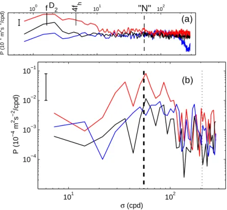
spectral domain (Fig. 5). In contrast with open ocean data (Fig. 1), the overall spectra of temperature-inferred w and ADCP-w poorly match for the North Sea data, especially near the semidiurnal frequency (Fig. 5a). Despite the small amplitudes, ADCP’s w-estimate is significantly exceeding noise levels. Only for the small periods of Fig. 3b some comparison is found between ADCP-w and temperature-inferred w, albeit mostly

25

for small-scaleN in the lower pycnocline, TN=420 s (Fig. 5b). It is noted that the best

spectral amplitude comparison for large-scale N is found between pycnocline tempera-ture variations and near-bottom ADCPw-estimate. ADCP’s w in the pycnocline shows larger amplitudes. This suggests that the bottom boundary layer drives these linear

OSD

Full Screen / Esc

Printer-friendly Version

Interactive Discussion

pycnocline motions, but that the enforcement of the pycnocline w(N) peak is highly non-linear and dominated by the first few periods (see Fig. 4d). Also in the entire record mean spectrum (Fig. 5a) lower-pycnocline temperature-inferredw correspond best with the level of near-bottom ADCP-w, but only for σ>5 cpd≈4 f_h,f_h=2Ωcosϕ the horizontal component of the Earth rotational vector Ω at latitude ϕ. This suggests

5

linear waves betweenN and this cut-off and non-linear motions for lower frequencies including tidal and inertial frequencies.

Estimates of turbulent diffusion indicate values of about K =6·10−4m2s−1across the pycnocline during the passage of the high-frequency [non-]linear wave, which gives values of 3–4·10−5m2s−1 integrated over a tidal period (van Haren et al., 1999). This

10

overall value is sufficient for nutrient transport generating the summer phytoplankton bloom, and these occasional near-N waves also govern the slow heating of the near-bottom layer during spring and autumn. Comparable K -values are observed on the Malin Shelf and attributed to non-linear high-frequency waves (Inall et al., 2000).

For all of the above evaluations of Eq. (1), <10% improvement is obtained using

15

instead of∂T (t)/∂z its time mean (Fig. 4). However, the influence of the time depen-dence is larger in a region where strongly turbulent non-linear “waves” or bores prevail, like on a FSC-slope.

3.2 Faeroe-Shetland Channel

Similar vertically striped, generally mode-1,w-motions are observed albeit in irregularly

20

occurring groups in the FSC and associated with non-linear wave trains moving up the slope (Hosegood and van Haren, 2004). In the FSC, vertical currents associated with high-frequency motions are larger (by a factor of 3–4) than in the central North Sea, commensurate the equally weaker stratification that supports them. As a result, one could “conclude” that |w|∼N−1, rather than ∼N−1/2, which is more common for

25

horizontal currents.

Despite the very accurate thermistor string (Table 2 for its characteristics) the vigor-ous motions cause substantial turbulent overturning, i.e. by definition not linear waves.

OSD

Full Screen / Esc

Printer-friendly Version

Interactive Discussion

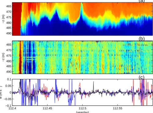
This explains the difficulty in evaluating Eq. (1) using these data and spikes are regu-larly large, especially in temperature-inferredw (Fig. 6c).

However, the frontal upwardw-jet, exceeding 0.1 m s−1, is detected by both inferred and direct measurements, which is surprising when compared with the first “wave” period of small-scale North Sea motions (Fig. 4d). The small phase lag of 30–60 s

5

between the differently observed jet in the FSC (Fig. 6c) is attributable to the ADCP’s beam spread in combination with thermistor string motions due to current drag. Regu-lar Regu-large-scale, indeed∼1500 s∼TN period, and occasionally very high frequency

mo-tions, are adequately described by Eq. (1). The best comparison with ADCP’s w is obtained using∂T (t)/∂z rather than its time mean, which implies that a non-linear term

10

is needed to dampen some of the high-frequency spiking, but in the vertical direction only. Unfortunately, the data do not allow the evaluation of horizontal non-linear terms, responsible for the (turbulent) spikes during other periods. The local turbulent diffusiv-ity is large,K ∼O(10−1m2s−1) (Hosegood and van Haren, 2004), but the passage is so rapid that the value integrated over a tidal period is similar to the one above that was

15

estimated for the North Sea.

4 Discussion

It has been shown that directw-observations describe realistic ocean phenomena that have horizontal length scales larger than an ADCP’s beam spread, being 10 m here. The present data do not [directly] represent free convection, but rather [non-]linear

in-20

ternal waves or frontal advection (cf. Fig. 4). A strong association between the motions’ periodicity and depth of maximum amplitude with stratification favours an explanation in terms of internal waves, e.g. Fig. 3b. This has been confirmed using Eq. (1), but it is found that this standard method to computew from T -data does not work in a tidal advection area like the North Sea or in an area where non-linear motions prevail over

25

linear [high-frequency] waves.

near-OSD

Full Screen / Esc

Printer-friendly Version

Interactive Discussion

bottom areas and that non-linear near-N motions dominate the internal “wave” spec-trum near its upper bound in the ocean interior may also explain the discrepancy in w-spectra from the Bay of Biscay (Fig. 1). Presumably, weakly non-linear waves likewise dominate the open ocean continuum as well, possibly as interfacial waves like in the North Sea, because the ADCP’s w-data exceed noise level and temperature-inferred

5

w at frequencies between tidal harmonics, e.g. between semidiurnal and fourth-diurnal bands in Fig. 1.

The lack of dominant linear high-frequency waves may explain the quarter-wave pe-riod discrepancy betweenT and w observations found by Hallock and Field (2005). It certainly explains East China Sea observations by Lee et al. (2006), who found 3 large

10

“waves” of depression before a group of about 10 higher frequency waves, just like in Fig. 3b. As for the North Sea observations presented here, the sudden change in phase difference between time derivative and vertical advection terms in Eq. (1) after the first two wave periods bears some resemblance with laboratory experiments on the generation of mode-2 internal waves following an intrusion in a linearly stratified

15

fluid (Amen and Maxworthy, 1980). Although no w-observations were presented by these authors, the gravitational collapse of a mixed region generated two mode-2 soli-tary waves followed by a train of constant amplitude mode-1 waves of approximately doubled frequency. When sufficiently strong, mode-2 waves can appear as closed contour “waves”, with importance for transporting material (Davis and Acrivos, 1967).

20

Here, they are only observed in limited form, at the top of the bottom-boundary layer (Fig. 3), and, peculiarly, [two] mode-1 waves precede mode-2 waves. More modeling is required to establish the generation of such waves, although it has been shown that mode-2 waves can [occasionally] follow a mode-1 wave breaking on a sloping shelf (Helfrich, 1992).

25

More modeling is also required to establish whether a non-zero limit value exists to diapycnal diffusivity across strong stratification, as suggested by the tidal mean value found in different regions presented here and which are apparently induced by high-frequency non-linear motions.

OSD

Full Screen / Esc

Printer-friendly Version

Interactive Discussion

Similarly, more modeling is required to establish the large discrepancy between di-rectly measured and temperature-inferred w at sub-inertial frequencies. Certainly, the assumption underlying Eq. (1) eliminates gyroscopic waves, which are prevalent in ho-mogeneous layers in the frequency range [0, 2Ω]. These waves show relatively large w that can be directly measured and which extend spectrally to about σ=4fh before

5

dropping into noise (van Haren and Millot, 2005). They are not measured by temper-ature sensors in homogeneous layers. In contrast in a stratified ocean, the internal wave band drops off for σ<4fh, but faster for temperature-inferred w than ADCP’sw

(Fig. 1a). Apparently also small-scale advection or eddies are not incorporated by Eq. (1), which gives the impression of a strict internal wave band consisting only of

10

tidal harmonic motions dropping off for σ<f , but which is unrealistic in terms of oceanic low and high-modew.

Acknowledgements. The assistance of the crew of R/V Pelagia is highly appreciated. I thank

T. Hillebrand for mooring preparation. Integrated North Sea Program (INP) and Processes above Continental Slopes (PROCS) were funded in part by the Netherlands Organization for

15

the advancement of Scientific Research (NWO).

References

Amen, R. and Maxworthy, T.: The gravitational collapse of a mixed region into a linearly strati-fied fluid, J. Fluid Mech., 96, 65–80, 1980.

Davis, R. E. and Acrivos, A.: Solitary internal waves in deep water, J. Fluid Mech., 29, 593–607,

20

1967.

Hallock, Z. R. and Field, R. L.: Internal-wave energy fluxes on the New Jersey Shelf, J. Phys. Oceanogr., 35, 3–12, 2005.

Helfrich, K. R.: Internal solitary wave breaking and run-up on a uniform slope, J. Fluid Mech., 243, 133–154, 1992.

25

Helfrich, K. R. and Melville, W. K: On long nonlinear internal waves over slope-shelf topography, J. Fluid Mech., 167, 285–308, 1986.

OSD

Full Screen / Esc

Printer-friendly Version

Interactive Discussion

Hosegood, P. and van Haren, H.: Near-bed solibores over the continental slope in the Faeroe-Shetland Channel, Deep-Sea Res. Pt. II, 51, 2943–2971, 2004.

Howarth, M. J.: The effect of stratification on tidal current profiles, Cont. Shelf Res., 18, 1235– 1254, 1998.

Inall, M. E., Rippeth, T. P., and Sherwin, T. J.: Impact of nonlinear waves on the dissipation of

5

internal tidal energy at a shelf break, J. Geophys. Res., 105, 8687-8705, 2000.

Krauss, W.: Methoden und Ergebnisse der Theoretischen Ozeanographie. II Interne Wellen. Gebrueder Borntraeger, Berlin, 248 pp., 1966.

Lee, J. H., Lozovatsky, I., Jang, S.-T., Jang, C. J., Hong, C. S., and Fernando, H. J. S.: Episodes of nonlinear internal waves in the northern East China Sea, Geophys. Res. Lett., 33, L18601,

10

doi:10.1029/2006GL027136, 2006.

van Aken, H. M., van Haren, H., and Maas, L. R. M.: The high-resolution vertical structure of internal tides and near-inertial waves, measured with an ADCP over the continental slope in the Bay of Biscay, Deep-Sea Res. I, 54, 533–556, 2007.

van Haren, H. and Millot, C.: Gyroscopic waves in the Mediterranean Sea, Geophys. Res. Lett.,

15

32, L24614, doi:10.1029/2005GL023915, 2005.

van Haren, H., Maas, L., Zimmerman, J. T. F., Ridderinkhof, H., and Malschaert, H.: Strong inertial currents and marginal internal wave stability in the central North Sea, Geophys. Res. Lett., 26, 2993–2996, 1999.

van Haren, H., Groenewegen, R., Laan, M., and Koster, B.: A fast and accurate thermistor

20

OSD

Full Screen / Esc

Printer-friendly Version

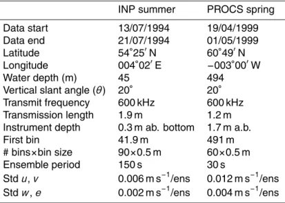
Interactive Discussion Table 1. RDI-broadband uplooking-ADCP mooring details. INP is in the central North Sea,

PROCS in the Faeroe-Shetland Channel.

INP summer PROCS spring Data start 13/07/1994 19/04/1999 Data end 21/07/1994 01/05/1999 Latitude 54◦25′N 60◦49′N Longitude 004◦02′E −003◦00′W Water depth (m) 45 494

Vertical slant angle (θ) 20◦ 20◦ Transmit frequency 600 kHz 600 kHz Transmission length 1.9 m 1.2 m Instrument depth 0.3 m ab. bottom 1.7 m a.b. First bin 41.9 m 491 m # bins×bin size 90×0.5 m 60×0.5 m Ensemble period 150 s 30 s

Stdu, v 0.006 m s−1/ens 0.012 m s−1/ens Stdw, e 0.002 m s−1/ens 0.004 m s−1/ens

OSD

Full Screen / Esc

Printer-friendly Version

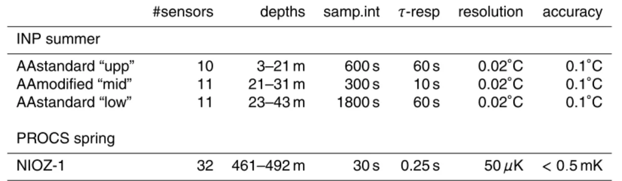
Interactive Discussion Table 2. Thermistor string mooring details. AA=Aanderaa, NIOZ=Netherlands Institue for Sea

Research design (van Haren et al., 2001). The modified AA-thermistor string has standard sensors that are connected to aluminium plates cut in the rubber tube that holds the entire string and strength member. This decreases the response time.

#sensors depths samp.int τ-resp resolution accuracy INP summer AAstandard “upp” 10 3–21 m 600 s 60 s 0.02◦C 0.1◦C AAmodified “mid” 11 21–31 m 300 s 10 s 0.02◦C 0.1◦C AAstandard “low” 11 23–43 m 1800 s 60 s 0.02◦C 0.1◦C PROCS spring NIOZ-1 32 461–492 m 30 s 0.25 s 50µK < 0.5 mK

OSD

Full Screen / Esc

Printer-friendly Version

Interactive Discussion Fig. 1. (a) Spectra ofw-data in the Bay of Biscay measured at 46◦43′N, 5◦24′W (H=1600 m),

using 75 kHz ADCP at 1040 m (black) and compared with instrumental, measurement noise (blue) andw inferred from ADCP’s temperature data at 1100 m using Eq. (1) with CTD-data to

estimate mean vertical gradient (red), partially after van Aken et al. (2007). The CTD-estimated buoyancy frequency (N) range is indicated with a horizontal line; the horizontal component of

the Coriolis force is indicated byf_hand discussed in Sect. 3.1. (b) Time series ofw-data in (a). (c) 1-d detail of (b) showing near-N oscillations.

OSD

Full Screen / Esc

Printer-friendly Version Interactive Discussion Longitude (°E) Latitude (°N)

Figure 2

Fig. 2. Mooring locations (•) in North Sea (INP), Faeroe-Shetland Channel (PROCS) and Bay

OSD

Full Screen / Esc

Printer-friendly Version Interactive Discussion (yearday) −z (m) (10−2 _{m s}−1₎ (a) 194 196 198 200 202 0 10 20 30 40 ₋₁ −0.5 0 0.5 1 −z (m) (b) 194.7 194.75 194.8 194.85 0 5 10 15 20 25 30 35 40 45 −z (m) (c) 200.45 200.5 200.55 20 25 30 35 40 45

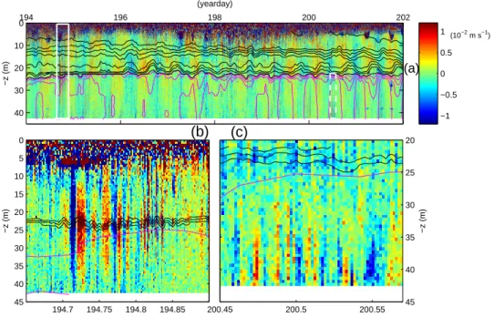
Fig. 3. Summertime INP time series. (a) Vertical current data with hourly smoothed

tempera-ture contours every 1◦C between 10–18◦C (black) and every 0.2◦C between 9.1–9.9◦C (purple). The solid rectangle indicates the period of panel (b), the dashed rectangle that of panel (c). (b) Detail of (a) with high-frequency waves near mid-depth and only one purple contour (9.5◦C), (c) Detail of (a) with high-frequency waves near the bottom and only one purple contour (9.3◦C). Note different z,t scales compared to (b). In (a–b) the brown band between 0 and about −7 m represents bad (surface reflection side-band) ADCP-data.

OSD

Full Screen / Esc

Printer-friendly Version Interactive Discussion 194 195 196 197 198 199 200 201 202 −2 0 2 x 10−3 ( oC s −1 ) (a) −2 0 2 x 10−3 ( oC s −1 ) (b) −5 0 5 x 10−5 ( oC s −1 ) (c) 194.6 194.7 194.8 194.9 −0.01 0 0.01 ( oC s −1 ) (yearday) (d)

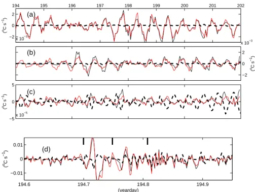
Fig. 4. Comparison of the two terms of Eq. (1) using INP-data. Left-hand side of Eq. (1) is

dashed, right-hand side is presented by a thin solid line with∂T (t)/∂z in black and its mean

in red. (a) Total time series, hourly averaged data at−12 m. (b) As (a), but at −20 m. (c) As (a), but at−30 m. (d) Raw, 5 min sampled T - and averaged w-data at −22.5 m for the detailed period of Fig. 3b. Three important transitional periods are indicated. Note the different scales compared with (a–c).

OSD

Full Screen / Esc

Printer-friendly Version Interactive Discussion 100 101 102 P (10 −2 m 2s −2 /cpd) D 2 f 4f h "N" (a) 101 102 10−4 10−3 10−2 10−1 P (10 −4 m 2 s −2 /cpd) σ (cpd) (b)

Fig. 5. W -spectra from summertime-INP ADCP-data at −22.5 m (red) and −39.5 m (black),

in comparison withw at −22.5 m inferred from temperature data using Eq. (1) (blue). (a) For

entire 8-d period. (b) For period of Fig. 3b between days 194.70 and 194.85. The dashed line indicates the buoyancy frequency corresponding to a period of 1600 s (∼ bottom boundary layer) and the dotted line indicates a period of 420 s (lower pycnocline).

OSD

Full Screen / Esc

Printer-friendly Version Interactive Discussion −z (m) (a) 465 470 475 480 485 490 −z (m) (b) 465 470 475 480 485 490 112.4 112.45 112.5 112.55 −0.1 −0.05 0 0.05 0.1 w (m s −1 ) (c) (yearday)

Fig. 6. W -test for frontal solibore in 5-h detail in FSC-data. (a) High-resolution temperature

measured using NIOZ-1. Values between [2, 8]◦C (blue–red). (b) Corresponding ADCP’s

w-data. Values between [−0.04, 004] m s−1 (blue–red). (c) W at 477 m from ADCP (black)

and inferred from temperature data using Eq. (1) and unsmoothed local vertical temperature gradient (blue), and time mean temperature gradient (red).