Chaotic Sampling, Very Weakly Coupling, and Chaotic Mixing: Three Simple Synergistic Mechanisms to Make New Families of Chaotic Pseudo Random Number Generators

HAL Id: hal-00258017

https://hal.archives-ouvertes.fr/hal-00258017v3

Preprint submitted on 8 May 2008

HAL is a multi-disciplinary open access

archive for the deposit and dissemination of

sci-entific research documents, whether they are

pub-lished or not. The documents may come from

teaching and research institutions in France or

abroad, or from public or private research centers.

L’archive ouverte pluridisciplinaire HAL, est

destinée au dépôt et à la diffusion de documents

scientifiques de niveau recherche, publiés ou non,

émanant des établissements d’enseignement et de

recherche français ou étrangers, des laboratoires

publics ou privés.

Chaotic Sampling, Very Weakly Coupling, and Chaotic

Mixing: Three Simple Synergistic Mechanisms to Make

New Families of Chaotic Pseudo Random Number

Generators

René Lozi

To cite this version:

René Lozi. Chaotic Sampling, Very Weakly Coupling, and Chaotic Mixing: Three Simple Synergistic

Mechanisms to Make New Families of Chaotic Pseudo Random Number Generators. 2008.

�hal-00258017v3�

ENOC 2008, Saint Petersburg, Russia, June, 30-July, 4 2008

CHAOTIC SAMPLING, VERY WEAKLY COUPLING, AND CHAOTING MIXING:

THREE SIMPLE SYNERGISTIC MECHANISMS TO MAKE NEW FAMILIES OF

CHAOTIC PSEUDO RANDOM NUMBER GENERATORS

René Lozi

Laboratoire J.A. Dieudonné – UMR du CNRS N° 6621, University of Nice-Sophia-Antipolis, Parc Valrose, 06108 Nice Cedex 02, France

and

Institut Universitaire de Formation des Maîtres Célestin Freinet-académie de Nice, University of Nice-Sophia-Antipolis, 89 avenue George V, 06046 Nice Cedex 1, France

rlozi@unice.fr

Abstract

We introduce and combine synergistically three simple new mechanisms: very weakly coupling of chaotic maps, chaotic sampling and chaotic mixing of iterated points in order to make new families of enhanced Chaotic Pseudo Random Number Generators (CPRNG).

The key feature of these CPRNG is that they use chaotic numbers themselves in order to sample and to mix chaotically several subsequences of chaotic numbers.

We analyze numerically the properties of these new families and underline their very high qualities and usefulness as CPRNG when series are computed up to 1013 iterations.

Key words

Chaos, pseudo random numbers, coupled maps. 1. Introduction

When a dynamical system is realized on a computer using floating point or double precision numbers, the computation is of a discretization, where finite machine arithmetic replaces continuum state space. For chaotic dynamical systems, the discretization often has collapsing effects to a fixed point or to short cycles [Lanford III, 1998; Gora, Boyarsky, Islam and Bahsoun, 2006].

In order to preserve the chaotic properties of the continuous models in numerical experiments we have introduced as a first one mechanism the very weak multidimensional coupling of p

one-dimensional dynamical systems which is

noteworthy [Lozi, 2006].

Moreover each component of these numbers belonging to _{ℝ are equally distributed over a} p

given finite interval J⊂ℝ . Numerical

computations show that this distribution is obtained with a very good approximation. They have also the property that the length of the periods of the numerically observed orbits is very large.

However chaotic numbers are not pseudo-random numbers because the plot of the couples of iterated points (xn, xn+1) in the phase plane shows up the map f used as one-dimensional dynamical systems to generate them.

A second simple mechanism is then used to hide the graph of this genuine function f in the phase

space

(

l

)

n l n x

x , +1 . The pivotal idea of this mechanism

is to sample chaotically the sequence

(

0, 1, 2,…, , 1,…

)

l n l n l l l x x x x x ₊ selecting l n x every time the value of m n

x is strictly greater than a threshold T ∈ J, with l ≠ m, for 1 ≤ l, m ≤ p .

A third mechanism can improve the

unpredictability of the chaotic sequence generated as above, using synergistically all the components of the vector X, instead of two. This simple third mechanism is based on the chaotic mixing of the p-1

sequences

(

, , ,…, , 1 ,…

)

1 1 1 2 1 1 1 0 x x xn xn+ x ,

(

, , ,…, , 2 ,…

)

1 2 2 2 2 1 2 0 x x xn xn+ x ,…,

(

, , ,…, , 1,…

)

1 1 1 2 1 1 1 0 − + − − − − p n p n p p p x x x x

x using the last one

(

0, 1, 2,…, , 1,…

)

p n p n p p p x x x x

x ₊ with respect to a given

partition r1, r2, …, rp-1 of J, to distribute the iterated

points.

In this paper we explore numerically the properties of these new families and underline their very high qualities and usefulness as CPRNG when series are computed up to 1013 iterations.

Generation of random or pseudorandom

numbers, nowadays, is a key feature of industrial mathematics. Pseudorandom or chaotic numbers are used in many areas of contemporary technology such as modern communication systems and engineering applications. Everything we do to achieve privacy and security in the computer age depends on random numbers. More and more European or US patents using discrete mappings for this purpose are obtained by researchers of discrete dynamical systems [Petersen and Sorensen, 2007; Ruggiero, Mascolo, Pedaci and Amato, 2006].

The idea of construction of chaotic

pseudorandom number generators (CPRNG)

applying discrete chaotic dynamical systems,

          = p x x X ⋮ 1

intrinsically, exploits the property of extreme sensitivity of trajectories to small changes of initial conditions, since the generated bits are associated with trajectories in an appropriate way [Bofetta, Cencini, Falcioni and Vulpiani, 2002].

Recently some authors proposed the use of the Arnol’d cat maps as a PNRG [Barash and Schchur, 2006].

The process of chaotic sampling and mixing of chaotic sequences, which is pivotal for these new families, works perfectly in numerical simulation when floating point (or double precision) numbers are handled by a computer.

It is noteworthy that the new models of very weakly coupled maps are more powerful than the usual formulas used to generate chaotic sequences mainly because only additions and multiplications are used in the computation process; no division being required. Moreover the computations are done using floating point or double precision numbers, allowing the use of the powerful Floating Point Unit (FPU) of the modern microprocessors (built by both Intel and Advanced Micro devices (AMD)). In addition, a large part of the computations can be parallelized taking advantage of the multicore microprocessors.

2. Very Weakly Multi-dimensional Coupling 2.1. Two-dimensional Coupled Symmetric Tent Map

First, we recall the basic equation of the coupled symmetric tent maps. In sections 2, 3 and 4 of this paper, we will consider only the symmetric tent map defined by

x a x

f_a( )=1− (2.1)

with the value a = 2, later denoted simply as f, even though others map of the interval (as the logistic map) can be used for the same purpose. The associated dynamical system [Sprott, 2003; Alligood, Sauer and Yorke, 1996] is defined by the equation on the interval J = [-1, 1]

n n ax

x ₊₁=1− (2.2)

Two tent maps are coupled in the following way, using a two dimensional coupling constant ε = (ε1, ε2)    − + = + − = + + ) ( ) ε 1 ( ) ( ε ) ( ε ) ( ) ε 1 ( n 2 n 2 1 n n 1 n 1 1 n y f x f y y f x f x _(2.3)

In this paper for the numerical studies we fix constant the ratio between ε1 and ε2. We chose to set it equal to 2.

1 2 2ε

ε =

(2.4)

However, different ratios can also lead to good results and be used since a multidimensional variable can be instrumental in the increasing of the number of dimensions of the systems.

The coupling constant ε varies from (0, 0) to (1, 1). When ε = (0, 0) the maps are decoupled, when ε = (1, 1) they are fully cross coupled. Generally, researchers do not consider very small values of ε (as small as 10-7 for floating point numbers or 10-14 for double precision numbers), because it seems that the maps are quasi decoupled with those values. Hence no special effect of the coupling is expected. In fact it is not the case and this very very small coupling constant allows the construction of very long periodic orbits, leading to sterling chaotic generators.

The dynamical system (2.3) can be described more generally by

( )

n

(

( n)

)

1 n F X A f X X ₊ = = ⋅ (2.5) with x X y   =   

,

_      = ) ( ) ( ) ( y f x f X f (2.6) and       − − = ) 1 ( ) 1 ( 2 2 1 1 ε ε ε ε A (2.7)

where F is a map of the square [-1, 1] x [-1, 1] = J2 into itself.

2.2 p-coupled Symmetric Tent Map

To improve the length of the period and the convergence of the invariant measure towards a given measure, we consider the dynamical system (2.5) in which p maps are coupled

with           = p x x X ⋮ 1 ,           = ) ( ) ( ) ( 1 p x f x f X f ⋮ (2.8) and                 = p p p 2 2 2 2 1 1 1 1 ε 1) -(p -1 ε ε ε ε ε 1) -(p -1 ε ε ε ε ε 1) -(p -1 ⋯ ⋯ ⋮ ⋮ ⋱ ⋮ ⋮ ⋮ ⋱ ⋮ ⋯ ⋯ A (2.9) with ε_i=_iε₁ i = 2, …, p (2.10)

As stated earlier, others choices are possible. In this case, F is a map of Jp into itself.

2.3 Uniform distribution of chaotic numbers We give some numerical results about chaotic numbers produced by 2-, 3- and 4-coupled maps which show that they are equally distributed over the interval J. In order to compute numerically an

approximation of the invariant measure [3] also called the probability distribution function PN (x)

linked to the one dimensional map f we consider a regular partition of M small intervals (boxes) of

J= 2 0 M i r −

∪

ri = [si , si+1[ , i = 0, M – 2 (2.11) rM-1 = [sM-1 , 1] (2.12) M i si 2 1+ − = i = 0, M (2.13) Its length is M s s_i+1− _i= 2 (2.14)

All iterates f (n)(x) belonging to these boxes are collected (after a transient regime of q iterations decided a priori, i.e. the first q iterates are neglected). Once the computation of N+ q iterates is completed, the relative number of iterates with respect to N/M in each box ri represents the value PN (si). The approximated PN (x) defined in this

article is then a step function, with M steps. As M may vary, we define

( )

i i N M r N M s P # 2 1 ) ( , = (2.15)

where #ri is the number of iterates belonging to the interval ri and the constant 1/2 allows the normalisation of P_M,N(x) on the interval J.

i i N M N M x P s x r P _, ( )= _, ( ) ∀ ∈ (2.16)

In the case of coupled maps, we are interested by the distribution of each component x1, …, x p of X rather than the distribution of the variable X itself in Jp. We then consider the approximated probability distribution function PN (x

j

) associated to one among several components of F(X) defined by (2.5) which are one-dimensional maps.

The discrepancies E1 (in norm L1) and E2 (in

norm L2) between

P

_,

(

x

)

iter disc N

N and the Lebesgue

measure which is the invariant measure associated to the symmetric tent map, are defined by

1 5 . 0 ) ( ) , ( _, 1 Ndisc Niter PN N x _L E iter disc − = (2.17) 2 5 . 0 ) ( ) , ( , 2 Ndisc Niter PN N x _L E = _{disc iter} −

(2.18)

Fig. 1 shows the error E₁(N_disc,N_iter) versus the number of iterates of the approximated distribution functions with respect to the first variable x1 for 2, 3 and 4-coupled symmetric tent map. Ndisc is fixed to 104, ε1 to 10-14, Niter varies from 10

5

to 1011 for the 2-coupled case and to 3.1012 for the 3 and 4-coupled one. -4,5 -4 -3,5 -3 -2,5 -2 -1,5 -1 -0,5 4 5 6 7 8 9 10 11 12 13 log10(Niter) lo g1 0 (E 1 ) 2 coupled equations 3 coupled equations 4 coupled equations

Figure 1. Error E1 for 2, 3 and 4-coupled

Symmetric Tent Maps. Computations done using double precision numbers (~14-15 digits), εi = i.ε1, ε1 = 10-14, Ndisc = 104. Initial values

1 0 x = 0.330000013113, 2 0 x = 0.338756413113, 3 0 x = 0.331353442113, 4 0 x = 0.333213583113.

Same results are obtained in norm L2.

The corresponding numerical results are displayed in Tab. 1 for E₁(N_disc,N_iter) for and Tab. 2 for

(

)

2

2(Ndisc,Niter)

E .

Remark: in order to made easier the comparison of the results, we display the square of the discrepancy

2 2

E instead of E2 itself, the discrepancy being

divided by 10 each time the number of iterations is multiplied by 10.

One can observe that for 3 and 4-coupled equations the convergence is excellent up to 3×1012 iterates. For 2-coupled equations the convergence seems lower bounded by a minimal error.

Niter ) , ( 1 Ndisc Niter E 2-coupled equation ) , ( 1 Ndisc Niter E 3-coupled equation ) , ( 1 Ndisc Niter E 4-coupled equation 105 _{0.25071335 0.25035328 0.2499133} 106 _{0.079655103 0.079437105 0.080739109} 107 _{0.025794703 0.025343302 0.025266304} 108 _{0.0081966502 0.0079505501 0.0080771501} 109 _{0.003147609 0.002513533 0.002562893} 1010 0.002171746 0.0007908719 0.00079702 1011 0.002055097 0.000257910 0.000252414 1012 _8.4195287.10-5 _7.8803383.10-5 3.1012 _5.0625114.10-5 _4.5317128.10-5

Table 1. Error E1 for 2, 3 and 4-coupled Symmetric

Tent Maps.

Niter ) , ( 2 2 Ndisc Niter E 2-coupled equation ) , ( 2 2 Ndisc Niter E 3-coupled equation ) , ( 2 2 Ndisc Niter E 4-coupled equation 105 0.100199 0.099820996 0.099610992 106 _{0.01006199 0.0098781898 0.01022057} 107 _{0.0010442081 0.0010014581 0.0010055967} 108 _{0.0001055816 9.8853067.10}-5 _{0.00010197872} 109 1.567597.10-5 1.0047459.10-5 1.0326474.10-5 1010 _7.3577797.10-6 _9.7251536.10-7 _9.9932242.10-7 1011 _6.6338453.10-6 _1.0434293.10-7 _1.0070523.10-7 1012 _1.116009.10-8 _9.6166733.10-9 3.1012 4.0443118.10-9 3.2530773.10-9 Table 2. Error 2 2

E for 2, 3 and 4-coupled Symmetric Tent Maps.

There is no significant difference between 3 and 4-coupled equations, the numerical experiments have to be pursued up to 1013 or 1014 in order to discriminate the results.

Equivalent results are obtained for the variables x2, x3or x4.

No periodic solutions are observed up to 3×1012 iterates (even up to 1013 iterates as tested in Sec. 4). This is a key point when producing chaotic numbers, because the use of a computer discretizes the phase space of a dynamical system, canceling (at least) its asymptotic properties. Every orbit is periodic according to the finite number of states (i.e., the number of double precision numbers belonging to Jp). However, if the period of the realized sequence is long enough, these properties reasonably survive as a chaotic transient.

2,0 4,0 _6,0 5 ,0 8 ,0 1 1 ,0 -5,0 -3,0 -1,0 1,0 lo g (E 1 ) log(N disc ) log (Niter ) -5--3 -3--1 -1-1

Figure 2. Error E1 for 3-coupled Symmetric Tent

Maps. Computations done using double precision

numbers (~14-15 digits) with respect to both

Niter and Ndisc, εi = i.ε1, ε1 = 10-14, Niter = 105 to

1012, Ndisc = 10 2 to 107. Initial values 1 0 x = 0.330000013113, 2 0 x = 0.338756413113, 3 0 x = 0.331353442113, 4 0 x = 0.333213583113.

In Fig. 2, we display the mutual influence of both Niter and Ndisc on the errors in L1 norm. The

results show a tremendous regularity. The corresponding numerical results are displayed in Tab. 3. Ndisc Niter ) , ( 1 Ndisc Niter E 102 ) , ( 1 Ndisc Niter E 103 ) , ( 1 Ndisc Niter E 104 105 _{0.023590236 0.074390944 0.25035328} 106 _{0.0077829878 0.024115036 0.079437105} 107 _{0.0027963003 0.0078734998 0.025343302} 108 _{0.00070102901 0.0024396098 0.0079505501} 109 _{0.00024907298 0.00078846501 0.002513533} 1010 _7.4041294.10-5 _{0.0002472693 0.0007908719} 1011 _2.821469.10-5 _8.540793.10-5 _{0.00025791013} 1012 1.4600127.10-5 3.2358931.10-5 8.4195287.10-5 Ndisc Niter ) , ( 1Ndisc Niter E 105 ) , ( 1 Ndisc Niter E 106 ) , ( 1 Ndisc Niter E 107 105 0.73832 1.810124 1.9801114 106 _{0.24974733 0.735708 1.809666} 107 _{0.079959311 0.25029673 0.7353684} 108 _{0.02518029 0.079508971 0.25000429} 109 _{0.008005619 0.025207567 0.079757051} 1010 0.0025136649 0.0079736449 0.025230797 1011 _{0.00080110625 0.002522144 0.0079771447} 1012 _{0.00025407246 0.00079907514 0.0025234708}

Table 3. Error E1 for 3-coupled Symmetric Tent

Maps with respect to both Niter and Ndisc. 2.4 Impact of the initial values on the results

It is well known that the choice of the seed of a PRNG is very important. Some seed can lead to the collapse of the period of the computed random numbers. In order to check if the choice of the initial condition (equivalent to the choice of the seed of a PRNG) is dramatically for the previous results, we have tested several series of different initial values.

Fig. 3 shows the distribution of the error E1 for

500,000 initial values for 4-coupled symmetric tent maps. The computations are done using double precision numbers (~14-15 digits),

εi = i.ε1, ε1 = 10 -14 , Niter = 10 6 , Ndisc = 10 2 . The initial values are selected following:

x10,k = -0.92712 + 10-7× k ,

x20,k = -0.9183636 + 10-7× 7k,

x30,k = -0.92576657 + 10-7× 13k,

x40,k = -0.92390643 + 10-7× 17k,

k = 1 to 500,000.

The distribution follows more or less a Gaussian distribution, maximal and minimal results are displayed in Tab. 4. Others series tested with several values of Ndisc give the same kind of results.

Ndisc = 10 2 Niter = 10 6 0 5000 10000 15000 20000 40 50 60 70 80 90 100110120130140 Error E1 x 10 -4 n u m b e r o f re s u lt s o u t o f 5 0 0 ,0 0 0 4-coupled equations

Figure 3. Distribution of the error E1 for 500,000

initial values for 4-coupled symmetric tent maps.

Ndisc 102 103 104

minE₁(N_disc,N_iter) 0.0040021 0.0207400 0.0751521

max _{( , )} 1 Ndisc Niter E 0.013872 0.0301160 0.0843841 min 2_{( , )} 2 Ndisc Niter E 0.0000275 0.0006769 0.0089217 max 2_{( , )} 2 Ndisc Niter E 0.0002834 0.001435 0.0110719

Table 4. Minimal and maximal values of the E1 and

2 2

E errors for 500,000 initial values for 4-coupled symmetric tent maps.

2.5 Independency of the chaotic subsequences generated by each component

In next section, we propose the chaotic sampling of the chaotic sequences generated by Eq. (2.5) to enhance the properties of this chaotic number generator. The key feature of these enhanced chaotic number generators being their use of chaotic numbers themselves in order to do the sampling process. The main idea leading to this particular sampling is that the series of chaotic

numbers produced by each component is

independent of the others.

We need before to verify this independency. Let consider now the coordinates of the iterated points X₀,X₁,X₂,⋯,X_n,X_n+1,⋯

of the multidimensional map F defined by (2.5). In order to check that they are uncorrelated, we plot every pair of coordinates of this sequence in the phase subspace (xl, xm) imbedded in the phase space Jp and we check if they are uniformly distributed in the square J2.

If no particular pattern is displayed and if the difference between the distribution of these points later called the correlation distribution function

CN (x,y) converges towards the uniform distribution

on the square when the number of iterations goes to the infinity, we can conclude the independency or the uncorrelation of the sequences of numbers generated by each component of the iterated points.

In order to compute numerically an

approximation of the correlation distribution function CN (x,y) we build a regular partition of M 2

small squares (boxes) of J2 imbedded in the phase subspace (xl, xm) ri,j = [si , si+1[ × [tj , tj+1[ , i, j = 0, M – 2 (2.19) rM-1,j = [sM-1 , 1] × [tj , tj+1[ , j = 0, M – 2 (2.20) ri,M-1 = [si , si+1[× [tM-1 , 1] , i = 0, M – 2 (2.21) rM-1,M-1 = [sM-1 , 1] × [tM-1 , 1] (2.22) M i si 2 1+ − = , M j tj 2 1+ − = , i, j = 0, M (2.23)

the measure of the area of each box is :

(

1

) (

1

)

2 2       = − ⋅ − + + M t t s s_{i i i i} (2.24)

Once N + q iterated points

(

m

)

n l n x

x , belonging to these boxes are collected the relative number of iterates with respect to N/M2 in each box ri,j represents the value CN (si,tj). The approximated

probability distribution function CN (x,y) defined in

this article is then a 2-dimensional step function, with M2 steps. As M can vary in the next sections, we define

( )

ij j i N M r N M t s C _, 2 , # 4 1 ) , ( = (2.25)

where #ri,j is the number of iterates belonging to the square ri,j and the constant 1/4 allows the

normalisation of _{( , )} , x y CMN on the square J 2_. j i j i N M N M x y C s t x y r C _, ( , )= _, ( , ) ∀( , )∈ _, (2.26)               = p n n n x x X ⋮ ⋮ 1

The discrepancies EC1 (in norm L1 between ) , ( , x y C iter disc N

N and the uniform distribution on the

square is defined by 1 25 . 0 ) , ( ) , ( _, 1 disc iter N N _L C N N C x y E = _{disc iter} − (2.27)

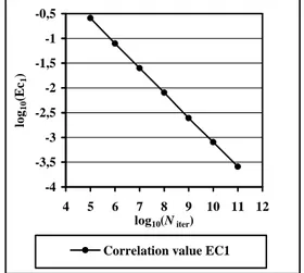
Fig. 4 shows the error _{( , )}

1 disc iter C N N

E versus the

number of iterated points of the approximated correlation function between the first and the second components (x1, x2) for the 4-coupled symmetric tent map. Moreover, every couple of components checked simultaneously gives the same results. -4 -3,5 -3 -2,5 -2 -1,5 -1 -0,5 4 5 6 7 8 9 10 11 12 log10(Niter) lo g1 0 (E c1 )

Correlation value EC1

Figure 4. Error EC1 for the first and the second components (x1, x2) of the 4-coupled symmetric tent map. Ndisc is fixed to 102 x 102, εi = i.ε1, ε1 = 10-14, Niter varies from 105 to 1011. Computations are done using double precision numbers (~14-15 digits). x10= 0.330, x 2 0= 0.3387564, x 3 0= 0.50492331, x 4 0= 0.0.

3. Chaotic Sampling of Chaotic Numbers

If we plot the chaotic numbers produced by any component xl , 1 ≤ l ≤ p of the p-dimensional dynamical system Eq. (2.5) in the phase space

(

l

)

n l n x

x , +1 , the iterated points show the graph of the

symmetrical tent map f used to define Eq. (2.5) (more exactly a graph with two lines having ε thickness). These numbers are not randomly produced. If we plot these points in the phase

spaces

(

l

)

n l n x x , ₊₂ ,

(

l

)

n l n x x , ₊₃ or

(

l

)

r n l n x x , ₊ they will display the graph of f (2), f (3) or f (r) (see Fig. 5). Hence someone knowing a sequence of few iterated points is able to find the initial value X0 of the dynamical system.

In order to hide the graph of the genuine function

f in the phase space

(

l

)

q n l n x

x , ₊ for any q, a pivotal idea is to sample chaotically the sequence

(

₀, ₁, ₂,…, , l ₁,…

)

n l n l l l _{x x x x}

x ₊ selecting x every time the nl

value of m n

x is greater than a threshold T, -1 < T < 1, with l ≠ m, for 1 ≤ l, m ≤ p .

The chaotically sampled subsequence

(

x₀,x₁,x₂,⋯,x_q,x_q+1,⋯

)

is defined as

] [

T,1 x iff x x m n l n q = ∈ (3.1)

Choosing T > 0.5 implies that the selected subsequence

(

x0,x1,x2,⋯,xq,xq+1,⋯

)

=

(

0, 1, 2,…, , 1,…

)

l p l p l p l p l p x x xq x q x ₊

is such that the difference between pq and pq+1 is always greater than a minimal value Km depending upon T. The graph of the chaotically sampled chaotic number is a mix of the graphs of all the f (r) for r > Km.

Figure 5. Graphs of the symmetric tent map f, f(2) and f(3) on the interval [-1,1].

As seen in Sect. 2.5 every pair of components

(

m

)

n l n x

x , of X₀,X₁,X₂,⋯,X_n,X_n+1,⋯ is

uncorrelated. Hence, the proposed chaotic sampling is a powerful tool to generate enhanced chaotic

numbers. Let _{( , )}

, x y

ACMN the autocorrelation

distribution function which is the correlation function CM_,N(x,y) (2.26) defined in the phase

space

(

l

)

n l n x

x , +1 instead of the phase space (x

l , xm). In order to control that the enhanced chaotic numbers

(

x₀,x₁,x₂,⋯,xq,xq₊₁,⋯

)

are uncorrelated, we plot them in the phase subspace

(

)

1

, n₊ n x

x and

we check if they are uniformly distributed in the square J2.

If no particular pattern is displayed and if the autocorrelation distribution function ACN (x, y)

converges towards the uniform distribution on the square when the number of iterations goes to the infinity, we can conclude that the knowledge of a sequence of iterated points do not allow finding the initial value X0 of the dynamical system.

Fig. 6 shows the values of

1 25 . 0 ) , ( ) , ( _,

1 disc iter N NSampl _L

AC N NSampl AC x y

E = _{disc iter} −

for a system of 4 coupled-equations for both the threshold values 0.98 and 0.998 of 4

n

x . The

enhanced chaotic numbers are produced by the first

component 1

n

x of the dynamical system.

-4,5 -4 -3,5 -3 -2,5 -2 -1,5 -1 -0,5 2 3 4 5 6 7 8 9 10 11

log10(NSampliter)

lo g10 (E A C 1 ) Threshold 0,98 Threshold 0,998

Figure 6. Error EAC1 for the first component x1, sampled by x4 for the threshold values 0.98 and 0.998 of the 4-coupled symmetric tent map. Ndisc=10×10, εi = i.ε1, ε1 = 10-14, NSampliter varies from 103 to 1010. Computations done using double precision numbers (~14-15 digits).

x10= 0.330, x20= 0.3387564, x30= 0.50492331, x40= 0.0. As the chaotic numbers are regularly distributed on the interval J, when T > 0.98 one chaotic number over approximately 100 is sampled, when T > 0.998 one chaotic number over approximately 1,000 is sampled. We call NSampliter the number of sampled points.

Figure 7. Difference between the autocorrelation distribution function ACNSAMPLDISC

(

x1n,x1n₊₁

)

and the

uniform distribution of the 4-coupled symmetric tent map sampled by x4 for the threshold value 0.998. Ndisc = 102×102, NSampliter= 1010, εi = i.ε1,

ε1 = 10-14. Initial values:

x10= 0.330, x20= 0.3387564, x30= 0.50492331, x40= 0.0.

Figure 8. Projection of the Fig. 7 on the plane

(

1

)

1 1 , n+ n x x .

Nevertheless the computing process is very fast. A desktop computer can produce more than 50,000,000 chaotic numbers per second, thus 50,000 iterated sampled points per second for T > 0.998. The sampling threshold 0.998 gives very good results.

The difference between the autocorrelation distribution function ACNSAMPLDISC

(

xn,xn₊₁

)

and the

uniform distribution is shown on Fig. 7 and its

projection on the phase subspace

(

)

1

, n₊ n x

x is shown

on Fig. 8.

Fig. 9 and Tab. 5 show E_AC1(N_disc,NSampl_iter) with respect to Ndisc

Nsampl_iter = 1010 0 0,0001 0,0002 0,0003 0,0004 0,0005 0,0006 0,0007 0,0008 0,0009 0 20 40 60 80 100 Ndisc lo g (E A C 1 )

4-coupled equations Threshold = 0.998

Figure 9. EAC₁(Ndisc,NSampliter) for the first component x1, sampled by x4 for the threshold value 0.998 of the 4-coupled symmetric tent map versus Ndisc, NSampliter = 1010, εi = i.ε1, ε1 = 10-14. Initial values x10 = 0.330, x20 = 0.3387564,

x30 = 0.50492331, x40 = 0.0.

Ndisc NSampliter EAC1(Ndisc,NSampliter)

10x 10 10,000,042,552 0.0000884451

40 x 40 10,000,042,552 0.000322549

100x 100 10,000,042,552 0.000798014

Table 5. EAC₁(Ndisc,NSampliter).

4 Chaotic Mixing and Chaotic Sampling of Chaotic Numbers

One can improve again the unpredictability of the chaotic numbers generated as above, using all the components of the vector X instead of one. For example for 4-coupled equations, the value of 4

n

x command the sampling process as follows

Let us set three threshold values T1, T2 and T3 -1 < T1 < T2 < T3 < 1 (4.1) we sample and mix together chaotically the sequences

(

, , ,…, , 1 ,…

)

1 1 1 2 1 1 1 0 x x xn xn+ x ,

(

, , ,…, , 2 ,…

)

1 2 2 2 2 1 2 0 x x xn xn+ x and

(

, , ,…, , 3 ,…

)

1 3 3 2 3 1 3 0 x x xn xn+ x defining

(

x0,x1,x2,⋯,xq,xq+1,⋯

)

by

]

[

[

[

[

[

     ∈ ∈ ∈ = 1 , , , 3 4 3 3 2 4 2 2 1 4 1 T x iff x T T x iff x T T x iff x x n n n n n n q (4.2) -4,5 -4 -3,5 -3 -2,5 -2 -1,5 -1 -0,5 2 3 4 5 6 7 8 9 10 11 Log10(NSampliter)

lo g1 0 (E A C 1 ) Threshold 0,98 Threshold 0,998 Thresholds 0,98 ; 0,987; 0,994 Thresholds 0,998 ; 0,9987; 0,9994

Figure 10. Error of E_AC1(N_disc,NSampl_iter) Ndisc=102×102, NSampliter= 103 to 1010, εi = i.ε1,

ε1=10-14.

Fig. 10 and Tab. 6 show the values of )

, (

1 disc iter

AC N NSampl

E for a system of 4

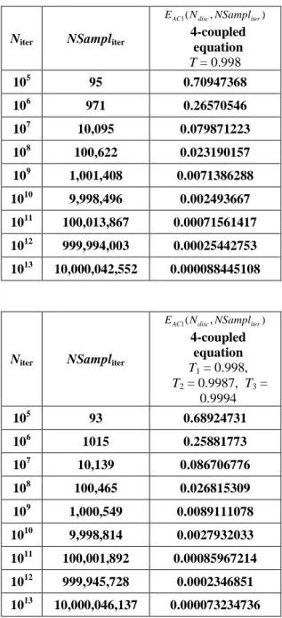
coupled-equations when the first component x1 is sampled by x4 for both the threshold values 0.98 and 0.998 and when the three components x1 , x2 , x3 are mixed and sampled by x4 for the threshold values T1 = 0.98, T2 = 0.987, T3 = 0.994 or T1 = 0.998, T2 = 0.9987, T3 = 0.9994.

Niter NSampliter

) , ( 1 disc iter AC N NSampl E 4-coupled equation T = 0.998 105 95 0.70947368 106 971 0.26570546 107 10,095 0.079871223 108 100,622 0.023190157 109 1,001,408 0.0071386288 1010 9,998,496 0.002493667 1011 100,013,867 0.00071561417 1012 999,994,003 0.00025442753 1013 10,000,042,552 0.000088445108

Niter NSampliter

) , ( 1 disc iter AC N NSampl E 4-coupled equation T1 = 0.998, T2 = 0.9987, T3 = 0.9994 105 93 0.68924731 106 1015 0.25881773 107 10,139 0.086706776 108 100,465 0.026815309 109 1,000,549 0.0089111078 1010 9,998,814 0.0027932033 1011 100,001,892 0.00085967214 1012 999,945,728 0.0002346851 1013 10,000,046,137 0.000073234736

Table 6. Error of EAC1(Ndisc,NSampliter) for a system of 4 coupled-equations when the first component x1 is sampled by x4 for the threshold value 0.998 and when the three components x1 , x2 , x3 are mixed and sampled by x4 for the threshold values T1 = 0.998, T2 = 0.9987, T3 = 0.9994.

5. Further improvements

As said in Sec. 2.1, we have only considered the symmetric tent map (2.1). We have now to consider others maps of the interval: non symmetric tent map, baker map. We have also to consider the coupling (2.5) with maps having different parameters values





















=

)

(

)

(

)

(

1 1 p a a

x

f

x

f

X

f

p

⋮

(5.1) ( m i

a∈ℝ being for example a general parameter

value characterizing the general baker map)

6. Conclusion

We have introduced and combined

synergistically three simple new mechanisms: very weakly coupling of chaotic maps, chaotic sampling and chaotic mixing of iterated points in order to make new families of enhanced Chaotic Pseudo Random Number Generators (CPRNG). The properties of these new families are explored numerically up to 1013 iterations. The numerical experiments give good results. Now other tests have to be performed in order to check their usefulness

as Chaotic PRNG. Others functions and

combination of functions have also to be explored in order to obtain

References

Alligood, K. T., Sauer, T. D., and Yorke, J. A. (1996). Chaos. An introduction to dynamical systems. Springer, Textbooks in mathematical sciences. New-York.

Barash, L., Shchur, L. N. (2006). Periodic orbits of the ensemble of Sinai-Arnold cat maps and pseudorandom number generation. Physical Review E. 73, Issue 3, pp.036701.

Boffetta, G., Cencini, M., Falcioni, M., Vulpiani, A. (2002). Predictability : a way to characterize complexity. Physics Reports. 356, pp. 367-474. Gora, P., Boyarsky, A., Islam, MD. S., Bahsoun, W. (2006). Absolutely continuous invariant measures that cannot be observed experimentally. SIAM J. Appl. Dyn. Syst. 5:1, pp. 84-90 (electronic). Lanford III, O. E. (1998). Some informal remarks on the orbit structure of discrete approximations to chaotic maps. Experimental Mathematics. Vol. 7, 4, pp. 317-324.

Lozi, R. (2006). Giga-Periodic Orbits for Weakly Coupled Tent and Logistic Discretized Maps.

(International Conference on Industrial and Applied Mathematics, New Delhi, december 2004). Modern Mathematical Models, Methods and Algorithms for Real World Systems. A.H. Siddiqi, I.S. Duff and O. Christensen (Editors). Anamaya Publishers. New Delhi, India. pp 80-124.

Petersen, M. V., Sorensen, H. M. (2007). Method of generating pseudo-random numbers in an electronic device, and a method of encrypting and decrypting electronic data. United States Patent. 7170997. Ruggiero, D., Mascolo, D., Pedaci, I., Amato, P. (2006). Method of generating successions of pseudo-random bits or numbers. United States Patent Application. 20060251250.

Sprott, J. C. (2003). Chaos and Time-Series Analysis. Oxford University Press. Oxford, UK.