HAL Id: hal-01114751
https://hal.archives-ouvertes.fr/hal-01114751
Submitted on 10 Feb 2015
HAL is a multi-disciplinary open access
archive for the deposit and dissemination of
sci-entific research documents, whether they are
pub-lished or not. The documents may come from
teaching and research institutions in France or
abroad, or from public or private research centers.
L’archive ouverte pluridisciplinaire HAL, est
destinée au dépôt et à la diffusion de documents
scientifiques de niveau recherche, publiés ou non,
émanant des établissements d’enseignement et de
recherche français ou étrangers, des laboratoires
publics ou privés.
climate-chemistry models with emphasis on the role of
the temporal variability
C. Déandreis, Yves Balkanski, J.L. Dufresne, A. Cozic
To cite this version:
C. Déandreis, Yves Balkanski, J.L. Dufresne, A. Cozic. Radiative forcing estimates of sulfate aerosol in
coupled climate-chemistry models with emphasis on the role of the temporal variability. Atmospheric
Chemistry and Physics, European Geosciences Union, 2012, 12 (12), pp.5583-5602.
�10.5194/acp-12-5583-2012�. �hal-01114751�
www.atmos-chem-phys.net/12/5583/2012/ doi:10.5194/acp-12-5583-2012
© Author(s) 2012. CC Attribution 3.0 License.
Chemistry
and Physics
Radiative forcing estimates of sulfate aerosol in coupled
climate-chemistry models with emphasis on the role of
the temporal variability
C. D´eandreis1, Y. Balkanski1, J. L. Dufresne2, and A. Cozic1
1Laboratoire des Sciences du Climat et de l’Environnement, UMR8212, IPSL, CEA-CNRS-UVSQ,
Gif-sur-Yvette Cedex, France
2Laboratoire de M´et´eorologie Dynamique, LMD/IPSL, CNRS-UPMC, Paris, France
Correspondence to: C. D´eandreis (cdeipsl@ipsl.jussieu.fr)
Received: 10 May 2011 – Published in Atmos. Chem. Phys. Discuss.: 30 August 2011 Revised: 23 March 2012 – Accepted: 26 March 2012 – Published: 26 June 2012
Abstract. This paper describes the impact on the sulfate aerosol radiative effects of coupling the radiative code of a global circulation model with a chemistry-aerosol mod-ule. With this coupling, temporal variations of sulfate aerosol concentrations influence the estimate of aerosol radiative im-pacts. Effects of this coupling have been assessed on net fluxes, radiative forcing and temperature for the direct and first indirect effects of sulfate.
The direct effect respond almost linearly to rapid changes in concentrations whereas the first indirect effect shows a strong non-linearity. In particular, sulfate temporal variabil-ity causes a modification of the short wave net fluxes at the top of the atmosphere of +0.24 and +0.22 W m−2 for the
present and preindustrial periods, respectively. This change is small compared to the value of the net flux at the top of the atmosphere (about 240 W m−2). The effect is more impor-tant in regions with low-level clouds and intermediate sulfate aerosol concentrations (from 0.1 to 0.8 µg (SO4) m−3in our
model).
The computation of the aerosol direct radiative forcing is quite straightforward and the temporal variability has little effect on its mean value. In contrast, quantifying the first indirect radiative forcing requires tackling technical issues first. We show that the preindustrial sulfate concentrations have to be calculated with the same meteorological trajec-tory used for computing the present ones. If this condition is not satisfied, it introduces an error on the estimation of the first indirect radiative forcing. Solutions are proposed to as-sess radiative forcing properly. In the reference method, the
coupling between chemistry and climate results in a global average increase of 8 % in the first indirect radiative forc-ing. This change reaches 50 % in the most sensitive regions. However, the reference method is not suited to run long cli-mate simulations. We present other methods that are simpler to implement in a coupled chemistry/climate model and that offer the possibility to assess radiative forcing.
1 Introduction
Aerosols affect the Earth’s climate system in two ways: di-rectly and indidi-rectly. Aerosols scatter sunlight and enhance the planetary shortwave (SW) albedo, through the so-called “aerosol direct effect”. Indirect effects relate to the modifica-tion of cloud radiative properties due to the change of aerosol concentration or properties by human activities. The increase of aerosol number enhances the cloud droplet number con-centration. Assuming a cloud liquid water content constant, it is responsible for the decrease of the droplet effective radius and the increase of the cloud reflectivity. Twomey (1974) was amongst the first to describe the so-called first indi-rect effect. It causes a negative radiative forcing on top of the atmosphere. Despite numerous studies, the uncertainty of the radiative forcing associated with this effect remains much larger than for greenhouse gases. The fourth IPCC report associated to the first indirect effect a negative forc-ing rangforc-ing from −0.2 to −1.9 W m−2(Forster et al., 2007) and stressed the importance of improving these estimates and
their associated uncertainties. Chen and Penner (2005) have analysed the uncertainty in the estimation of the first indirect aerosol effect due to emissions, chemical transport model, aerosol size distribution, cloud nucleation parameterization, and different clouds properties. The aerosol burden calcula-tion, the cloud fraccalcula-tion, and the representation of the prein-dustrial aerosol state (size distribution and mass concentra-tion) are the main sources of uncertainty. Chen and Pen-ner (2005) warn about the use of off-line simulations that could cause additional sources of uncertainty since they use a monthly average aerosol number concentration and argue for a fully coupled GCM, which would give a better estimate of the interactions between aerosols, clouds and radiation.
Part of the difficulty of assessing the aerosol effects on climate comes from their high variability. Aerosols have het-erogeneous emission sources and a relatively short lifetime (from day to several weeks) that explains their strong varia-tions in space and time.
Because of this high spatial variability, aerosol effects on climate should not only be assessed at the global scale but also region by region. High temporal variability of aerosol is induced by their large difference in size and the many pro-cesses that affect their properties (nucleation, coagulation, sedimentation, wet deposition, humidity growth. . . ). Varia-tions in meteorological fields induce to a large degree the temporal variability in aerosol properties, and there is strong interest to consider the full interactions between them by us-ing coupled climate-chemistry models.
This coupling is expected to introduce non-linearities. Al-though the direct radiative effect is almost a linear func-tion of aerosol concentrafunc-tion for a given cloud cover, non-linearities could be introduced by the change in time of the relative position of clouds and aerosols. The first indirect effect is non-linear, starting with the relationship between cloud droplet number concentration (CDNC) and aerosol concentration. In global models, this relationship may be de-scribed using empirical parameterizations that specify the CDNC as a function of the aerosol mass density (Boucher and Lohmann, 1995; Lohmann and Feichter, 1997; Roefols et al., 1998) or the aerosol number concentration (Jones et al., 1994; Menon et al., 2002; Suzuki et al., 2004), or us-ing physically-based parameterizations (Chuang et al., 1997; Abdul-Razak and Ghan, 2002; Nenes and Seinfeld, 2003) in which the CCN activation and the droplets formation pro-cesses are described prognostically. In all cases, aerosol tem-poral variability will modify the first indirect effect estima-tion through the non-linearity of the different parametrisa-tions. Other non-linearities influence the calculation of the first indirect effect, such as the relationship between cloud droplet size and cloud droplet number or between cloud op-tical thickness and cloud droplet size.
Several modelling groups have included interactive aerosols in their model and have performed many studies with this model configuration (e.g. Jones et al., 2001; Reddy et al., 2005; Roeckner et al., 2006). But, to our knowledge,
none of these studies include on-line radiative forcing calcu-lation taking into account the aerosol temporal variability. In effect, estimating radiative forcing with such a model con-figuration is not obvious and needs complex technical devel-opment. This limit leads several research groups to elaborate alternatives to the radiative forcing concept: the “radiative perturbation” (Penner et al, 2006); the “quasi-forcing” (Rot-stayn and Penner, 2001), the “ fixed SST forcing” (Hansen et al., 2002) and the “forcing with stratosphere and troposphere adjustment” (Shine et al., 2003). Lohmann et al. (2010) have evaluated such alternatives compared to radiative forcing. However, radiative forcing is a powerful diagnostic tool for studying climate perturbations. Then, we propose here to tackle this issue and elaborate solutions to compute tradi-tional radiative forcing.
To simplify analyses and focus on the introduction of aerosol temporal variability, aerosol/cloud interactions are treated in a simple way: only sulfate is considered in this per and we used an empirical formula for the activation pa-rameterisation. The methods presented in this paper are not valid for models using a mechanistic activation scheme. They are also not suited to analyse radiative forcing that directly impacts meteorological fields like the cloud lifetime effect or the semi-direct effect.
After a brief presentation of LMDZ GCM features and the aerosol parameterization in the model, a description of the main choices concerning the implementation of aerosol con-centrations and radiative effects (Sect. 2) is given. In Sect. 3, weaknesses, strengths and estimates are presented for the two main methods used until now to account for direct and first indirect effects in the LMDZ GCM. We also propose an esti-mate of the change in short-wave net fluxes due to aerosol temporal variability. In the last part of the paper, we ad-dress the question of computing radiative forcing in a cou-pled model. Two solutions to perform simultaneously radia-tive forcing calculation with interacradia-tive chemistry are pro-posed. We discuss their strengths and weaknesses consider-ing their technical performance and their accuracy concern-ing radiative forcconcern-ing estimates.
2 Methodology 2.1 Model description
In this study, we used the Laboratoire de M´et´eorologie Dy-namique general circulation model LMDZ (Hourdin et al., 2006) with a resolution of 3.75◦in longitude, 2.5◦in latitude
and 19 hybrid sigma coordinate levels extending from the surface up to 3 hPa. Climatological sea surface temperatures and sea-ice fractions are used as boundary conditions to the model.
The dynamical part of the LMDZ code is based on a finite-difference formulation of the transport primitive equations and resolves the large-scale advection every six minutes.
The physical part of the model includes the most relevant subgrid-scale physical processes such as the turbulent mix-ing in the boundary layer, and is computed with a time step of thirty minutes. Deep convection is parameterized us-ing the Emmanuel scheme (1991). Clouds are represented through a log-normal probability distribution function of subgrid scale total (vapor and condensed) water (Bony and Emmanuel, 2001). Effects of mountains (drag, lifting, grav-ity waves) are accounted for using state-of-the-art schemes (Lott, 1999). The land surface processes are parameterised through a bucket model. Radiative transfer is calculated us-ing a two-stream approximation, dividus-ing the radiation in an upwelling and a downwelling flux. The parameterization is based on the scheme of Fouquart and Bonnel (1980) in the solar spectrum (SW) and on an updated version of Mor-crette (1991) in the terrestrial part.
The direct and first indirect aerosol effects are included in LMDZ radiative calculations in the SW spectrum following closely the work of Quaas et al. (2004) with minor modifica-tions.
To facilitate the analysis, this study focused on the sulfate component of the aerosol. The optical thickness, τa, single
scattering albedo, ωa, and particle asymmetry parameter, ga,
are used by the radiative code to derive the direct effect. A Mie scattering model with the refractive index of Toon et al. (1976) for ammonium sulfate was used to compute the sulfate optical properties of each aerosol, mode taking into account aerosol size distribution. For the particles in the sol-uble mode, we used the hygroscopic growth factors of Martin et al. (2004) to account for the change in particle diameters due to water absorption.
The first indirect effect depends on the cloud optical thick-ness which varies with cloud droplet size and number. In the model, cloud optical thickness is parameterised in terms of cloud droplet effective radius (re)and of the cloud liquid
wa-ter path (W ), in each layer (Stephens, 1978):
τ =3 2
W reρwater
(1)
The cloud droplet effective radius, re, is related to the
volume-mean cloud droplet radius (rd)in our model by the
relationship: re=1.1 rd,and the volume-mean cloud droplet
radius for liquid water clouds is calculated assuming spheri-cal particles: rd= 3 s qlρair 4 35ρwaterNd (2)
where qlis the cloud liquid water mixing ratio, ρairis the air
density, ρwater is the density of liquid water, and Nd is the
cloud droplet number. Nd(cm−3)is diagnosed from sulfate
mass concentration, ms(µg (SO4)m−3), using the empirical
formula of Boucher and Lohmann (1995) (formula “D”).
Nd=10a0+a1log(ma) (3) cdnc =f(msulf) 0 50 100 150 200 250 300 350 400 450 0 2 4 6 8 10 msulf (µgSO4/m 3 ) c d n c ( c m -3) BL adjusted BL orig Net flux
Fig. 1. Relationship between clouds droplet number (cm−3)and
the sulfate concentrations (µg SO4m−3) from the Boucher and Lohmann (1995) D formula, with the original empirical constant (dashed) and with the adjusted empirical constant of Quaas and Boucher (2005) (solid line).
We replace the original values of the empirical constants (a0=2.21 and a1=0.41) by the re-adjusted values from
Quaas and Boucher (2005) who used POLDER space instru-ment retrievals (a0=1.7 and a1=0.2). Figure 1 presents the
“Boucher and Lohman” parameterisation for both the origi-nal and newer sets of empirical constants. With these new constants, the cloud droplet number sensitivity to aerosol op-tical depth perturbation is quite well represented in LMDZ-INCA compared to the observation (Quaas et al., 2009). To avoid unrealistic droplet number concentrations, especially in regions of small sulfate concentrations, Ndis restricted to
be within a range from 20 to 1000 droplets per cm−3. 2.2 Aerosol concentrations
The LMDZ model has been used in two different configura-tions that only differ by the way aerosol concentration is con-sidered: prescribed in one case (off-line configuration) and coupled with the INCA chemistry model in the other case (on-line configuration).
2.2.1 Aerosol off-line configuration
In the first configuration, referred to as “aerosol off-line”, the aerosol concentration fields are prescribed with a given frequency (month, day. . . ). These concentration fields have been computed and have been stored from previous simula-tions, including the transport and chemistry of aerosols and gases (see below). This method has been implemented in sev-eral GCM (IPCC, 2001) and has been used in many stud-ies (e.g. Haywood et al., 1997; Mitchell and Johns, 1997; Boer et al., 2000; Dai et al., 2001; Dufresne et al., 2005). This method was initially implemented in LMDZ by Quaas et al. (2004) and by default the sulfate concentrations are prescribed monthly. The “instantaneous radiative forcing”
(Hansen et al., 1997) is easy to estimate: one needs to com-pute the radiative fluxes two times at each time, one with per-turbed aerosol concentration and one with reference aerosol concentration. The radiative forcing is the difference between these two radiative fluxes.
2.2.2 Aerosol on-line configuration
In this configuration, referred as “aerosol on-line”, the chem-istry processes, the aerosol concentration and the meteoro-logical variables are fully coupled at each time step (30 min). The meteorological trajectory is influenced by sulfate con-centration and the sulfur chemistry is influenced by the me-teorological variables. The chemistry model is the Interac-tion with Chemistry and Aerosols (INCA); it consists of the sulfur cycle scheme (Schulz, 2007) and the CH4-NOx
-CO-O3 chemical scheme describing the background chemistry
of the troposphere (Hauglustaine et al., 2004). Sulfate con-centration and size distribution are calculated at each time step by integrating surface and in-situ emissions, wet and dry deposition processes (Schulz et al., 1998; Guelle et al., 1998a, b), humidity growth (Gerber, 1985), chemical reac-tions (Boucher et al., 2002) and transport. The chemical transformation of the gaseous sulphur species requires oxi-dants either in the gas-phase or in the liquid-phase. The sul-fur chemistry implemented in INCA is similar to the one de-scribed in Boucher et al. (2002). The oxidant fields are es-timated in INCA as part of the dynamic chemistry scheme. DMS and its product DMSO are oxidised using the actual concentrations of OH and NO3. SO2 is transformed to
sul-fate by H2O2and O3 in cloud liquid water. The formation
of sulfate is limited by the acidity formed in the oxidation process within cloud droplets. SO2 is also oxidised in the
gas-phase. Gaseous H2S and aerosol methane sulphonic acid
(MSA) are also included as minor species of the sulphur cy-cle. The mass of sulfate produced through these reactions is directly injected into the soluble accumulation mode. The nu-cleation mode is not treated explicitly, hence, there is no new particle formation in this size range and the very fine parti-cles are not represented. The mass median diameter (MMD) of sulfate depends upon the mixing of the ratio of sulfate formation from clouds and via gas phase oxidation. Further-more, the MMD varies as deposition takes place since large particles will be preferentially scavenged by sedimentation and below cloud scavenging.
2.3 Forcings
The study has been done for the present-day period (per-turbed conditions) and radiative forcing is assessed rela-tive to the preindustrial one (unperturbed condition). Sulfate, SO2and DMS emissions come from the AEROCOM project
emissions inventory (http://aerocom.met.no/Welcome.html) (Dentener et al., 2006). Natural emissions (DMS from ocean; sulfate and SO2from volcanoes) are kept unchanged between
preindustrial and present-day periods. Only anthropogenic emissions are modified.
The aerosol concentrations fields computed in the on-line simulations are averaged and used in the off-line runs. This ensures that in both on-line and off-line simulations, the monthly mean aerosol concentration are exactly the same.
Each simulation presented in the paper consists of a ten-year snap-shot including one spin-up ten-year. The last nine ten-years of each simulation are used for the radiative fluxes analy-sis. This nine-year duration allows reducing the noise due to internal model variability compared to the effect of anthro-pogenic forcing.
3 The radiative impact of aerosols and the effect of the temporal variability
In this section, the radiative forcing or aerosol radiative effect are presented for both the on-line and off-line configuration of the model. Table 1 details the setup used for each exper-iment presented in this paper using these two methods. The global values of these estimates are compared, as well as their geographical distributions. Then, we analyse the effect of the temporal variability of sulfate concentrations on radiative net fluxes.
3.1 Aerosol computed on-line
Two simulations have been performed using the “aerosol on-line” configuration of the model. They differ only by the SO2
emissions. For both simulations, greenhouse gas concentra-tions, sea surface temperature (SST) and sea ice fraction are fixed to present-day conditions. For gaseous chemistry, re-active gas emissions are kept to their 2000 levels. In the first simulation, natural plus preindustrial SO2emissions are used
whereas in the second simulation, natural plus present-day anthropogenic emissions are used. Below, we will refer to the preindustrial fields of the first simulation with the subscript “PI” and the present-day fields with the subscript “PD”.
The radiative perturbation (1FV)of anthropogenic sulfate
is computed as the difference of short-wave net fluxes (FV)
at the top of the atmosphere between the present-day and the preindustrial aerosol emissions (the subscript “V” indicates that fluxes have been computed including the instantaneous variability of aerosol concentrations).
1FV=FV PD−FV PI (4)
This radiative perturbation differs from an instantaneous ra-diative forcing because present-day and preindustrial net fluxes are estimated for two different atmospheric trajecto-ries after the atmospheric column (troposphere and strato-sphere) has had time to adjust. It is identical to the “fixed SST radiative forcing” defined by Hansen et al. (2002). This diagnostic tool includes both direct and first indirect effects. With this model version, it is not possible to study each effect separately. Fluxes include the two effects.
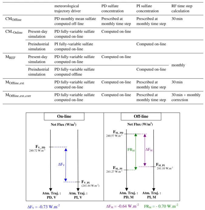
Table 1. Description of the experiments presented in this paper. The first column specifies which sulfate fields are used to drive the
mete-orological trajectory of the simulation; the 2nd and 3rd columns describe the type of aerosol used to calculate net fluxes at the top of the atmosphere and radiative forcing. The last column specifies the time step at which the radiative forcing is computed from radiative net fluxes. PD refers to present-day, PI to preindustrial.
meteorological PD sulfate PI sulfate RF time step trajectory driver concentration concentration calculation CMOffline PD monthly mean sulfate Prescribed at Prescribed at 30 min
computed off-line monthly time step monthly time step CM-Online Present-day PD fully-variable sulfate Computed on-line
simulation computed on-line
Preindustrial PI fully-variable sulfate Computed on-line simulation computed on-line
MREF Present-day PD fully-variable sulfate Computed on-line
monthly simulation computed on-line
Preindustrial PD fully-variable sulfate Computed on-line simulation computed offline
MOffline ext PD fully-variable sulfate Computed on-line Prescribed at 30 min
computed on-line monthly time step
MOffline ext corr PD fully-variable sulfate Computed on-line Prescribed at 30 min + monthly
computed on-line monthly time step correction
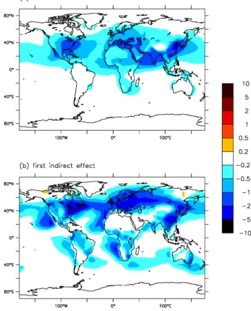
FM_PI 241.10 W.m-2 FM,_PD 240.57 W.m-2 FV_PI (241.44 W.m-2 ) ∆FV = -0.73 W.m-2 Net Flux (W/m2) ∆FM FRM FM,_PI 241.27 W.m-2 FV,_PD 240.72 W.m-2 Atm. Traj. : PD, V Atm. Traj. : PI, V ∆FV Atm. Traj. : PD, M Atm. Traj. : PI, M Net Flux (W/m2) FRM = - 0.70 W.m -2 ∆FM = -0.64 W.m-2 On-line Off-line
Fig. 2. Representation of the radiative perturbation (1F ) and radiative forcing (RF) calculated from simulations performed with the on-line
and off-line model configuration. For each case, both axes indicate that the fluxes are obtained for two different atmospheric model trajectories depending on the sulfate concentration: present-day or preindustrial ones. For the on-line configuration, the “V” annotation indicates that variable sulfate concentrations are used; as the “M” annotation referred to monthly mean concentration for the off-line configuration.
Values of FV PD, FV PI and 1FV are indicated in Fig. 2.
The global annual mean value of the radiative perturbation is −0.73 W m−2.
If we focus now on the geographical distribution of this ra-diative perturbation, the pattern that one may expect from the aerosol geographical distribution is not discernable and the
figure shows a noisy pattern (Fig. 3). This signal is due to nat-ural variability. The mean cloud distributions of the two sim-ulations are slightly different due to internal variability and this difference strongly impacts the radiative fluxes at the top of the atmosphere. The signal/noise ratio could be improved with long simulations of a hundred years, but the computing
Fig. 3. Difference between the short wave top-of-atmosphere net
fluxes (in W m−2)computed with present day and with preindus-trial sulfate emissions. The on-line configuration of the model is used.
time for the chemistry-aerosol module is prohibitive for such long runs.
3.2 Aerosol computed off-line
The same two simulations have been performed using the off-line configuration of the model. The prescribed aerosol concentrations are kept constant during each month and are set to the monthly mean value of the aerosol concentra-tions previously obtained with the on-line simulaconcentra-tions. This ensures that in both on-line and off-line simulations, the monthly mean aerosol concentrations are exactly the same. The fluxes computed with prescribed monthly mean aerosol concentration have the subscript “M”.
Figure 2 compares the shortwave net fluxes of the off-line configuration (FM PD, and FM PI)to those of the
on-line simulation (FV PD and FV PI). With this configuration,
the radiative perturbation (1FM)amounts to −0.64 W m−2.
It is 12 % higher than the value obtained when sulfate con-centration is computed on-line (−0.73 W m−2). In addition, the off-line configuration allows us to easily compute the radiative forcing of aerosols for both the direct and indi-rect effect of the aerosol (e.g. Quaas et al., 2004). The to-tal radiative forcing (sum of direct and first indirect effects) amounts to −0.70 W m−2. It is close to the radiative pertur-bation (1FM= −0.64 W m−2). This result is consistent with
Hansen et al. (2002), who obtained that the radiative pertur-bation for fixed SST is close to the instantaneous radiative forcing for non-absorbing aerosols such as sulfate.
The direct effect value is −0.31 W m−2, whereas the
in-direct effect reaches −0.39 W m−2. The simulated direct ra-diative forcing is very close to the mean value derived in the AEROCOM project of −0.35 ± 0.15 W m−2 (Schulz et al., 2006). This value also lies inside the 90 % confidence inter-val (−0.4 ± 0.2 W m−2)reported in the 4th IPCC assessment report (Forster et al., 2007). The first indirect radiative forc-ing straddles the lowest part (in absolute value) of the
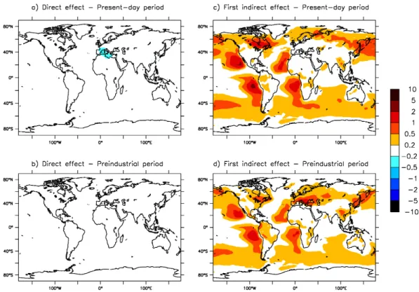
val-Fig. 4. Radiative forcings (W m−2)estimated with the off-line
con-figuration of the model for present-day, sulfate emissions: (a) direct effect (b) 1st indirect effect.
ues reported in the 4th IPCC report [−0.2 to −1.9 W m−2] (Forster et al., 2007). This low value of the first indirect effect comes mainly from the use of new constants a0 and
a1in the Boucher and Lohmann microphysics relationships
(Eq. 3). Quaas and Boucher (2005) showed that with their set of constants, simulated cloud droplet number decreases and the first indirect effect radiative forcing is divided by a factor 2. Dufresne et al. (2005) corroborate this finding in a study on climatic impact of sulfate aerosol performed with the IPSL coupled model that also shows the importance of low level clouds over continents.
Figure 4 shows the direct and first indirect aerosol radia-tive forcing. As expected, sulfate results in a cooling of the surface and displays a very heterogeneous distribution. The direct radiative forcing is strongly correlated to the emission sources. Values up to −5 W m−2can be reached in some in-dustrial regions. The patterns of the first indirect effect are correlated to both emission sources and cloud cover. Some regions in north latitudes show a positive first indirect effect. It comes from a decrease of SO2emissions by biomass
3.3 Effect of the sulfate temporal variability on the radiative fluxes
The radiative net fluxes of the on-line and off-line simula-tions may differ because of the frequency at which aerosol concentrations vary (prescribed every month in one case, computed every time step in the other case) but also because of the different meteorological trajectory between the two simulations. In the off-line method, the meteorological tra-jectory is influenced by the monthly mean sulfate concention, whereas in the on-line method, the meteorological tra-jectory responds to the effect of instantaneous concentrations (Fig. 2).
In this part of the study, the effect of the aerosol temporal variability has been isolated from the effect of the meteoro-logical trajectories and then analysed.
3.3.1 Method
The effect of the temporal variability is studied by compar-ing two simulations which only differ by the frequency at which the sulfate concentration is updated: every model time step (30 min) for the simulation is referred to as “VAR sim-ulation” and every month in the case of the simulation is re-ferred to as “MONTH simulation”. The average concentra-tions fields and the meteorological trajectory are the same for the 2 simulations; therefore the difference in the mean aerosol distribution can not be the reason of the difference between off-line and on-line runs.
For the VAR simulation, the aerosols are computed on-line as presented in Sect. 3.1. The MONTH simulation is run off-line with respect to the meteorological trajectory of the VAR simulation (temperature, pressure, wind, humidity, cloud fraction, LW path,. . . ). Then, the only difference in the MONTH simulation comes from the use of monthly sulfate concentrations that are used to compute aerosol and cloud radiative properties and radiative fluxes.
Two sets of VAR and MONTH simulations have been performed for present-day and preindustrial sulfate emis-sions. Preindustrial simulations have also been performed off-line with respect to the meteorological trajectory that is based on the present-day, fully-variable, sulfate aerosol retroaction. Then, the meteorological trajectory is exactly the same in the preindustrial and in the present-day simulations. The only difference is the anthropogenic emission of sulfate aerosols. We examine the change in net fluxes at the top-of-atmosphere between the experiments VAR and MONTH for the present day (FV PD−FM PD)and the preindustrial
peri-ods (FV PI−FM PI). Net fluxes are computed each 30 min and
monthly averaged for each simulation. Differences between the VAR and MONTH experiments are calculated from these monthly mean net flux values. The net fluxes resulting from this experiment are schematically presented in Fig. 5. The effect of the meteorological trajectory is null.
FV, PI 241. 40 W.m-2 FM,_PD 240.48 W.m-2 FV_PD – FM_PD = +0.24 W.m-2 FV_PI – FM_PI FM,_PI 241.18 W.m-2 FV,_PD 240.72 W.m-2 Atm. Traj. : PD, V FV_PD – FM_PD Net Flux (W/m2) FV_PI – FM_PI = + 0.22 W.m-2 Reference RFM RFV
Fig. 5. Representation of the difference of radiative net fluxes
cal-culated between the VAR (sulfate concentration computed each 30 min with INCA) and the MONTH (sulfate concentration pre-scribed each month) experiments. All simulations have been per-formed with the same physical forcings in order to get exactly the same meteorological trajectory: the present-day one with sulfate variability.
3.3.2 Global and regional results
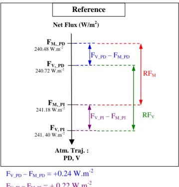
Figure 5 indicates the values of the shortwave net fluxes at the top-of-atmosphere for the two simulations VAR and MONTH and for the two periods. Globally, temporal vari-ability of sulfate concentration increases these net fluxes by +0.24 W m−2 for the present-day conditions and by +0.22 W m−2for the preindustrial ones. The regional distri-bution of this change for present day and preindustrial con-ditions is shown in Fig. 6; the impact of the direct effect (Fig. 6a and b) and the first indirect effect (Fig. 6c and d) are separated. With the exception of a few model grid points, the temporal variability leads to an increase of the total net fluxes (direct and first indirect effects) at the top of atmo-sphere for the two periods: preindustrial and present day. The changes in total net fluxes are within the interval −0.5 and +2.5 W m−2. However, as it is shown in Fig. 6a and b,
the direct effect has a negligible role, it tends to slightly de-crease net fluxes. The inde-crease of net fluxes results mainly from the first indirect effect. More precisely, this increase is linked to the shape of the relationship between the number concentration of cloud droplet Ndand the sulfate
concentra-tion ms. Consider Nd,M to be the number concentration of
Fig. 6. Difference of the top-of-atmosphere fluxes (W m−2)between the simulation in which the aerosol concentration varies at each time step (VAR experiment) and the simulation in which the concentration remains constant, prescribed to the monthly mean values (MONTH experiment) for present day sulfate emissions (top) and preindustrial sulfate emission (below). Impact of the sulfate first indirect effect (left) and the sulfate direct effect (right) are presented separately.
in the MONTH experiment. By construction, this value stays unchanged throughout the month. Let’s consider now, Nd,V,
the number concentrations obtained from the instantaneous sulfate concentrations in the VAR experiment. Because this relationship grows asymptotically when sulfate concentra-tion increases, the monthly mean of Nd,Vvalues will be less
than the Nd,Mvalue. Since net fluxes decrease when the
num-ber of cloud droplets increases, the monthly mean net fluxes computed in the experiment VAR, FVis greater than the
av-erage net fluxes FMcomputed from the monthly mean sulfate
concentration.
3.3.3 Analysis
Three main variables contribute to the radiative effect of aerosol: the fraction of low level clouds, their liquid water content, and the sulfate concentration. Figure 7 displays the cloud liquid water content and the percentage of the liquid water from low-level clouds. The presence of low clouds shows the same pattern as the changes in fluxes at the top of the atmosphere caused by the variability of sulfate con-centrations (Fig. 6c and d). In upwelling regions the change in flux at the top of the atmosphere reaches 1 to 2.5 W m−2 in present-day conditions. Coastal regions west of South and North America together with coastal regions west of Africa
are more affected than others by the variability of aerosol concentrations. In contrast, over Indonesia and India, the im-pact of the sulfate temporal variability is weak even though the liquid water content is much higher than over the other regions discussed. In these areas, clouds are situated at much higher altitudes (Fig. 7b). Finally, above dry regions without clouds, there is no indirect effect and hence no effect of the sulfate concentration’s variability.
The time average value of the sulfate concentration is shown in Fig. 8. Regions with low to intermediate sulfate concentration appear to be more sensitive to the aerosol tem-poral variability than regions with high sulfate concentra-tion. This effect can be seen over Europe, for instance. Net fluxes differ substantially in preindustrial conditions when sulfate concentrations are low (Figs. 6d and 8b), whereas the difference vanishes under present- day conditions (Figs. 6c and 8a). This effect can also be seen in South-East Asia.
The slope of the relationship between cloud droplet con-centration (Nd) and sulfate concentration (ms) of the first
indirect effect (Fig. 1) explains the difference of net fluxes between polluted and unpolluted regions. In unpolluted re-gions a small change in sulfate concentrations corresponds to a large change in cloud droplet number, whereas in pol-luted regions higher-level sulfate will result in small changes in cloud droplet number.
Fig. 7. (a) Cloud liquid water path (g m−2)for all the clouds and
(b) percentage of this liquid water path in low level clouds (P >
850 hPa).
We identified in our model a concentration threshold of 0.8 µg (SO4)m−3 above which temporal changes in sulfate
concentrations have little impact on net fluxes. The regions where this threshold is exceeded are: China, Europe and the east coast of the United States which all are areas downwind of the main industrialized regions. Other regions with high sulfate are located downwind of natural volcanic emission regions. For theses concentrations levels, the aerosol tempo-ral variability do not affect the top-of-atmosphere net fluxes. In contrast, the effect of aerosol temporal variability is large for intermediate sulfate concentrations (between about 0.1 and 0.8 µg (SO4) m−3)over remote regions.
In regions devoid of sulfate (concentration less than 0.1 µg (SO4)m−3), the first indirect effect is close to zero.
An example for such a region is South America, where the liquid water content is high, low-level clouds are abundant but sulfate levels are very small for the present day.
We chose six regions to show how different cloud and sul-fate concentrations fare affected differently by sulsul-fate tem-poral variability: the Pacific Ocean, the Atlantic Ocean, the southern part of South America, India, Indonesia and con-tinental Europe (Table 2). For each region, the liquid water content, the mean sulfate concentrations for present day and
Fig. 8. Annual mean of the sulfate load (mg (SO4) m−2)for present
day (a) and preindustrial periods (b).
preindustrial and the change in flux for present and prein-dustrial conditions are reported in Table 3. The comparison of preindustrial and present-day conditions confirms the sen-sitivity of radiative fluxes in regions of low level clouds to intermediate sulfate concentration. Vertical profiles of cloud liquid water content and preindustrial and present-day sul-fate concentrations are also displayed for these six regions (Fig. 9). Intermediate levels of sulfate concentrations are reached at the height of the low-level clouds. The maxi-mum sulfate concentration is reached above the low-level clouds’ altitude. The first indirect effect shows a marked non-linearity for these intermediate concentration levels (Fig. 1). This is one of the reasons for the strong sensitivity of the first indirect effect to the variability of sulfate in the presence of low-level clouds.
4 Calculation of the radiative forcing for on-line simulations
The estimate of radiative perturbation (defined in Sect. 3.1) needs very long simulations to reduce the noise due to natu-ral variability. Thus, this approach is not suitable for transient
Table 2. Geographical coordinates of the 6 regions that were used for the analysis shown in Fig. 7: (1) South Atlantic Ocean along the
West Coast of Africa (referred as AO-WAf), (2) North Pacific Ocean along the West Coast of North America (referred as PO-WNA); (3) the southern part of South America (South Am.); (4) India (India); (5) Indonesia Islands (InIs); (6) Europe (Eu).
R´egion WAf WNA Am. Sud Inde InIs Eu
Latitude 0–35◦S 10–40◦N 37–45◦S 6–25◦N −15◦S–0 35–60◦N Longitude 20◦W–15◦E 150–110◦W 66–72◦W 70–85◦E 130–165◦E 60–110◦E
Table 3. Cloud liquid water path (LWP in g m−2), percentage of this LWP in low-level clouds (%), sulfate load (mg (SO4)m−2)for present
and preindustrial periods, short waves top-of-atmosphere net flux difference (W m−2)between the VAR and MONTH experiments for present (1NFpr)and preindustrial (1NFpi) for the 6 regions targeted in Fig. 7: (1) South Atlantic Ocean along the West Coast of Africa (referred as AO-WAf), (2) North Pacific Ocean along the West Coast of North America (referred as PO-WNA); (3) the southern part of South America (South Am.); (4) India (India); (5) Indonesia Islands (InIs); (6) Europe (Eu).
Region LWP % LWP Present-day 1NFpr Preindustrial 1NFpi (g m−2) low-level sulfate (W m−2) sulfate (W m−2)
cloud (mg (SO4) m−2) (mg (SO4) m−2)
WAf 46.3 69.1 2.5 0.72 1.2 0.52 WNA 71.3 49.7 4.0 0.84 1.8 0.63 Am Sud 125.7 50 0.74 0.06 0.49 0.10 Inde 61.5 12.4 9.5 0.05 1.2 0.09 InIs 84.3 4.0 5.5 0.08 4.9 0.09 Eu 74.6 51.6 6.6 0.05 1.5 0.43
climate simulations. In addition, radiative forcing is a pow-erful diagnostic tool to compare the radiative impact of dif-ferent perturbations (aerosol, greenhouse gases, land use. . . ) and different aerosol types (sulfate, black carbon, organic carbon, etc). For these reasons, we propose several methods to compute aerosol radiative forcing for on-line simulations in the next section. Their relevance is discussed with respect to the computation time needed and to their precision. These methods have been developed for models using an empirical parameterization of the cloud droplet number concentration.
4.1 A direct extension of the radiative forcing computation method used for off-line simulations In the aerosols’ off-line configuration, the radiative forcing is simply computed as the difference, at each time step, be-tween the radiative fluxes computed with two aerosol con-centration fields: the actual concon-centration and a reference concentration, here chosen as the preindustrial one. These two fields are monthly mean values and remain constant dur-ing the whole month. One can directly apply this method for on-line configuration: the actual concentration is now the aerosols’ concentration calculated on-line by the INCA chemistry model and then varying at each time step. The preindustrial concentration is unchanged and still prescribed to its monthly mean value. This method is called, Moffline ext,
which stands for: extended off-line method (Table 1). The modification of the direct effect due to the change of aerosol concentration between present-day and preindustrial
conditions results in a difference of net fluxes at the top of the atmosphere that amounts to −0.32 W m−2. It is very close to the value of the direct radiative forcing obtained with the off-line method (−0.31 W m−2, Sect. 3.2). Computing sulfates interactively increases the difference of net fluxes at the top of the atmosphere by 3 % relative to the off-line method when these concentrations are read in. The geographical distribu-tion of these two fields is also very similar (Fig. 10a and c). Industrial regions where SO2emissions sources are located
are more sensitive to the temporal variability of aerosol. The non-linearity due to the variation with time of the sulfate con-centration is weak. It is consistent with the direct net flux changes analysed in Sect. 3.3
The modification of the first indirect effect due to the change of aerosol concentration between present-day and preinsustrial conditions results in a difference of net fluxes at the top of the atmosphere estimated at −0.17 W m−2. This value differs by 60 % compared to the radiative forcing ob-tained with the off-line method (−0.39 W m−2, Sect. 3.2). The geographical difference of these two fields (Fig. 10b) is positive almost everywhere, the highest values being in re-gions where low-level clouds are abundant (Fig. 10d). It is worth noticing that these regions are generally remote from the main SO2source regions and therefore are found where
the sulfate atmospheric load is small.
A sensitivity test has been performed in which 30 min preindustrial sulfate fields have been prescribed instead of monthly mean values. Results are very close to those of the initial extended off-line method showing that this difference
Fig. 9. Annual mean vertical profile of the cloud liquid water content (mg m−3), and of the sulfate content (in µg (SO4)m−3)for present day (SO4-PR) and preindustrial emissions (SO4-PI). 6 regions are considered, from top to bottom: (1) South Atlantic Ocean along the West Coast of Africa; (2) North Pacific Ocean along the West Coast of North America; (3) the southern part of South America; (4) India; (5) Indonesia Islands; (6) Europe.
Fig. 10. Radiative forcing calculated from the extended off-line method for: (a) sulfate direct effect (W m−2), (b) sulfate 1st indirect effect (W m−2). Difference of radiative forcings between the off-line extended method and the off-line method: (c) sulfate direct effect (W m−2),
(d) sulfate 1st indirect effect (W m−2). The statistical signifiance of the difference was tested at the 95 % confidence level using a bootstrap
method. Regions where the difference is statistically significant are indicated with dots. The scales of the top row maps are in the range [−10; +10 W m−2], whereas the values for the bottom row maps (that represent differences in radiative forcings) vary between [−2:+2] or [−5:+5] W m−2.
does not come from the use of monthly versus instantaneous aerosol concentrations.
Nevertheless, this simple method presents a major incon-sistency: the sulfate concentration field for the present day is computed on-line in the model, varies at each time step, and is linked to the meteorology of the simulation. In contrast, the preindustrial field does not vary with time and has no link with the actual meteorology. It has been obtained off-line from a previous simulation with different transport fields, dif-ferent timing for precipitation and clouds, and hence differ-ent timing for the scavenging of aerosols by clouds. This may have an important impact as the first indirect effect is strongly non-linear and the radiative forcing computed at each time step. At any given time, present day sulfate concentrations can be lower than preindustrial values, causing a positive first indirect effect estimate. These positive values of the first in-direct effect would not appear if the radiative forcing was computed from month mean net fluxes instead of from the instantaneous ones.
In this simple method, the aerosol concentration difference between the preindustrial and present periods has two distinct origins: the sulfate emissions and the variability of the atmo-sphere. The first effect is the one that we want to estimate. The second effect is unwanted and may have a large ampli-tude To avoid this inconsistency, both aerosol fields need to vary with time in a consistent manner, and therefore need to be computed with the same meteorological fields.
4.2 A reference method to compute the first indirect radiative forcing
In order to have a reference estimate of the indirect radiative forcing for on-line simulation, we compute the aerosol con-centration for present-day and preindustrial emissions with two very same meteorological trajectories. For both periods, the aerosol temporal variability is accounted for, the mete-orological trajectories are the same, hence the only differ-ence is the aerosol emission and the impact of the respective aerosol concentration fields on the radiative fluxes (Table 1). The approach is the same as the one described in Sect. 3.3.1. The simulations used here are the “VAR” experiments with
Fig. 11. (a) Reference method (MREF)radiative forcing of the first indirect effect (W m−2); (b) difference of radiative forcing between the reference method (MREF)and the off-line method (CMOffline). The statistical signifiance of the difference was tested at the 95 % confidence level using a bootstrap method. Regions where the dif-ference is statistically significant are indicated with dots.
present-day and preindustrial sulfate emissions. The prein-dustrial simulation is performed off-line with respect to the meteorological trajectory that is based on the present-day, fully-variable aerosol retroaction.
The instantaneous radiative forcing (RFV)is directly the
difference between the net flux at the top of the atmosphere with present-day emissions (FV PD) and with preindustrial
emissions (FV PI):
RFV=FV PD−FV PI (5)
The first indirect radiative forcing computed using this method is −0.36 W m−2, a little less than using the off-line
method (−0.39 W m−2) where averaged sulfate
concentra-tion fields are used. The first indirect effect (Fig. 11a) shows a very similar spatial distribution than the one obtained with the off-line method (Fig. 4b). The first indirect effect is more negative over Europe, the United-States and East Asia, and less negative over the boreal forests and in the eastern part of the ocean basins (Fig. 11b). The difference (estimated with a non-parametric bootstrap test) is statistically significant at
Fig. 12. Impact on surface temperature of coupling chemistry and
climate: difference of temperature anomaly (1T = TPD−TPI) be-tween on-line (1TV)and off-line configuration (1TM). The statis-tical signifiance of the difference was tested at the 95 % confidence level using a student test. Regions where the difference is statisti-cally significant are indicated with dots.
the 95 % confidence level in most regions. These changes are only due to the frequency at which aerosols vary (monthly in the off-line case and 30 min in the reference case). The dif-ference of meteorological trajectory between the redif-ference method and the off-line one does not affect the result (not shown).
Given that the largest differences of radiative forcing be-tween the two methods are over continents (Europe and North America), one could expect that although the SSTs are fixed, these differences of radiative forcing will have an impact on surface temperature over these regions. To distin-guish the real effect of temporal variability on temperature from the noise due to natural variability of climate, 50-yr simulations have been performed with off-line and on-line model configurations and for present-day and preindustrial periods. The difference of temperature over continents be-tween the two periods has been estimated for both config-urations of the models (1TV=TV PD−TV PI and 1TM=
TM PD−TM PI)and then compared. Globally, the difference
(1TV−1TM)amounts to −0.07◦C. Regionally, the signal is
within the interval [−0.9, 0.8]◦C and is not well correlated with radiative forcing (Fig. 12). We conclude from this test that the temporal variability of aerosol does not affect surface temperature fields.
With this method, we get a reference estimate of the first indirect radiative forcing including sulfate temporal variabil-ity. However, the multiple calls needed that use a lot of CPU make it impractical to use for routine simulations. Thus, we now propose two alternatives to compute aerosol radiative forcing in on-line simulations. They rely on the results of Sect. 4.1 that showed that the same meteorological fields are needed to compute both present-day and preindustrial con-centrations.
Table 4. Monthly mean (M), standard deviation of daily values (STD) and ratio (M/STD) of the factor FV PI−FM PIused to correct the radiative forcing of the “extended off-line method”.
JAN FEB MAR APR MAY JUN JUL AUG SEP OCT NOV DEC
M 0.274 0.232 0.189 0.186 0.221 0.226 0.260 0.237 0.241 0.220 0.228 0.251 STD 0.038 0.061 0.028 0.032 0.030 0.041 0.035 0.031 0.041 0.060 0.087 0.041 M/STD 0.13 0.26 0.15 0.17 0.13 0.15 0.13 0.13 0.17 0.27 0.38 0.16 RFM-Offline-ext= - 0.17 W.m-2 RFOffline-ext Net Flux (W/m2) FV, PD (240.72 W.m-2 ) FM,_PI (240.89 W.m-2 ) RFCORR = - 0.40 W.m-2 FM,PI - FV,PI= - 0.23 W.m-2 Net Flux (W/m2) FM,PI-FV,PI FM,_PI’ (240.78 W.m-2) FV,_PI’ (241.02 W.m-2 ) Atm. Traj. : (PD, V) Atm. Traj. : (PD, V)’ FV,_PI (241.02 W.m-2) RFCORR
Fig. 13. Schematical representation of the error in the radiative
forc-ing estimation computed from 2 sulfate fields which do not satisfy the criteria of having consistent meteorological fields. Correction with the “FM,PI−FV,PI” term estimated in the Sect. 5.5. The fluxes do not include the impact of direct effect. Only the change due to the first indirect effect is taken into account.
In the first alternative method (Sect. 4.3), we propose to correct the error introduced on net fluxes by the use of “in-consistent” aerosol fields (one constant during the whole month; one varying at each time step). The correction is based on the difference between net fluxes calculated using pre-calculated monthly preindustrial concentrations and us-ing 30 min preindustrial concentrations. Both preindustrial simulations are performed with the same meteorological tra-jectory. In the second alternative case (Sect. 4.4), we propose to estimate preindustrial sulfate concentration from present-day values. This ensures that both present and preindustrial sulfate concentrations are consistent with the meteorological trajectory of the simulation.
4.3 Correction of off-line/on-line biaisis
Computing preindustrial and present-day aerosol concentra-tions with two different meteorological trajectory results in an underestimation of 60 % of the first indirect radiative forc-ing (see Sect. 4.1). This “off-line/on-line” error corresponds to the term “FM,PI−FV,PI” (Fig. 13). This difference of net
Fig. 14. Difference of the radiative forcing of the 1st indirect
ef-fect calculated from the extended off-line method corrected with the 1NFPI term and that one calculated in the reference method (experiment VAR) in W m−2. The statistical signifiance of the dif-ference was tested at the 95 % confidence level using a bootstrap method. Regions where the difference is statistically significant are indicated with dots. Color bar of the first map varies from −10 and +10 W m−2, whereas values of the second map (difference) vary from −2 and +2 W m−2.
fluxes is due to the use of monthly vs. varying aerosol con-centrations. It amounts to −0.23 W m−2. Its geographical
distribution is displayed in Fig. 6b.
This error has a low day to day variability (Table 4). Then, we propose to assess monthly mean values of the error and use them to correct the monthly mean radiative forcings com-puted with the extended off-line simulation. Finally, the cor-rection consists in summing up the term “FM,PI−FV,PI” and
the biased radiative forcing RFoffline ext(Fig. 13):
RFoffline ext corr=RFoffline ext+FM,PI−FV,PI (6)
The direct radiative forcing remains unchanged compared to the estimation of the extended method off-line as any correc-tion are applied for this effect. For the first indirect effect, the corrected radiative forcing amounts to −0.41 W m−2. It
is 13 % less than the value calculated in our reference sim-ulation. The difference of radiative forcing calculated with this method and with the reference method is presented in Fig. 14. A slight overestimation of the first indirect effect (more negative) concerns a major part of the globe: only a few grid points in the North of Europe, the East of the United States, and in South Africa present an underestimation. This
Fig. 15. Correlation between the present-day sulfate concentration and the preindustrial one for 2 grid points (Paris and Tunisia) and 2 months
(January and July). The blue line represents the expected values of the actual by the preindustrial instantaneous ratio, considering it is the same as the ratio of monthly mean concentrations. Slopes indicate the values of the monthly mean ratio.
overestimation is statistically significant at the 95 % confi-dence level (bootstrap test).
Compared to the reference method (Sect. 4.1), the global error (−0.05 W m−2, 13 %) is slightly higher that the one computed from monthly averaged concentration fields (−0.03 W m−2, 8 %) with the off-line methods and MONTH
experiment. However, these values are low, and this method largely improves regional patterns (Fig. 14 versus Fig. 11b). The residual error is mainly due to a residual difference of meteorological trajectories: the inconsistence related to the calculation of sulfate concentration has been corrected, but the terms RFonline ext and “FM,PI−FV,PI” have been
es-timated from two different meteorological trajectories (see Fig. 13). Secondly, the hypothesis for this case is not per-fectly matched as the “FM,PI−FV,PI” term presents a small
variability.
Finally, this method is valid for aerosol studies but not for more complex cases in which several forcings are simultane-ously modified (climate simulation).
4.4 Approximation of the on-line aerosol preindustrial concentration
For this method, we expect that at a given time, for a sim-ilar meteorology, the ratio of preindustrial by actual instan-taneous concentrations is the same that the ratio of monthly mean concentrations:
At a given time t of a given month:
[SO4]pi,t
[SO4]pr,t
= [SO4]pi,month [SO4]pr,month
=preindustrial aerosol fraction (7)
Figure 15 shows that the variability of the instantaneous sul-fate concentration ratio is not completely caught by this ap-proach. However, one can get a rough estimate using this hy-pothesis.
In this method, the on-line configuration of the model is used. The preindustrial concentration field is calculated in multiplying the present-day aerosol concentration field (computed interactively in INCA) by the “preindustrial aerosol fraction”. The fraction is prescribed monthly. It is ob-tained from preindustrial and present sulfate fields that have been computed in previous simulations using the chemical-transport version of LMDZ-INCA.
Fig. 16. (a) Difference of radiative forcing between the method
using an approximation of the on-line preindustrial concentration and the extended off-line method for the direct effect (in W m−2);
(b) difference of radiative forcing between the method using an
ap-proximation of the on-line preindustrial concentration and the refer-ence method for the first indirect effect (in W m−2). The statistical signifiance of the difference was tested at the 95 % confidence level using a bootstrap method. Regions where the difference is statisti-cally significant are indicated with dots.
The direct radiative forcing amounts to −0.31 W m−2. It is very close to the values obtained with the off-line method (Sect. 3.2) and the extended off-line method (Sect. 4.1). The geographical distribution of the direct effect displays the same patterns that those obtained in the two other methods (see Fig. 16a for the difference with the extended off-line method). Only the regions of high sulfate concentrations are impacted.
The first indirect effect amounts to −0.36 W m−2
that matches up to the value of the reference method (−0.36 W m−2). Figure 16b shows the remaining differences in the geographical distribution. As for the other tested meth-ods, this difference is statistically significant (bootstrap test at the 95 % confidence level) in most regions. The differ-ence of patterns obtained between this method and the ref-erence method is close to the one obtained between the off-line method and the reference method (Fig. 11b). Using this
Fig. 17. Zonal mean of the difference of first indirect radiative
forc-ing (W m−2)of the off-line method (black) and the preindustrial sulfate concentration approximation method (red) compared to the reference method.
last method improves spatial patterns (Fig. 17), especially in regions of northern high latitude.
The remaining error in the estimate of the first indirect ef-fect radiative forcing is caused by how we approximate the preindustrial aerosol concentration fields.
4.5 Comparison of the results
All tested methods give very similar estimates of the direct radiative forcing but significative differences for the first in-direct effect. Figure 18 compares the performance of the tested methods to compute the first indirect radiative forc-ing (mean bias and error on the spatial pattern). Estimates of the root mean squared error and feasibility of each method are also summarised in Table 5.
Even though the method based on the approximation of the preindustrial sulfate concentration leads to the best re-sult regarding the mean bias, the extended off-line method with correction represents best the spatial pattern of the first indirect effect (comparison to the reference method). This method presents also the lowest root mean squared error. Re-garding the technical feasibility and ability to perform cli-mate studies, the method based on the approximation of the preindustrial sulfate concentration is by far the best method since it is simple to implement, relatively cheap computation-ally (even though preliminar chemistry-transport simulations are needed to compute the monthly mean aerosol fraction), and enables us to analyze several perturbations simultane-ously.
This last method has been implemented in the Earth Sys-tem Model of the Institut Pierre Simon Laplace (IPSL) and will be used for climate simulations including aerosols stud-ies.
Fig. 18. Comparison of biases on the estimation of the first indirect radiative forcing computed with the four tested methods and relative
to the reference method: off-line method (red), extended off-line method (green); corrected extended off-line method (cyan) preindustrial sulfate concentration approximation method (blue). Taylor diagram (left) presents the performance of methods to represent the spatial pattern of the first indirect effect (including standard deviation, correlation and centered root mean squared error). Right: scatter plot compares the mean bias and the standard deviation of the error for each method.
Table 5. Estimation of the error on the root mean squared error (RMSE) of the first indirect radiative forcing for the different methods
presented in this paper. The REF method is used as reference. “No RF” indicates that the method does not enable radiative forcing assessment. The second row “feasibility” is related to the technical feasibility of the method.
MREF CMOffline CM-Online MOffline ext MOffline ext-corr MSulf-PI-approx
RMSE 0 0.18 No RF 0.27 0.09 0.16
feasibility no yes yes yes yes yes
5 Conclusions
The impact of coupling a climate model to a chem-istry/aerosol model has been addressed using the LMDz general circulation model and the chemistry-aerosol mod-ule INCA. This coupling is in agreement with the actual trend of a more integrated Earth System Model for study-ing climate. With this model configuration, simulations in-clude a complete feedback between climate and aerosols. The cloud/aerosol interaction is computed in LMDZ using an empirical parameterization and considers sulfate as the only aerosol type in this study. The conclusion would be similar for a more complex representation of aerosol. Ab-sorbing aerosols would introduce additional non-linearities through the semi direct effect (modification of the meteoro-logical conditions of the atmosphere). However, they have no effects on the CDNC/Na relationship that is the main source of non-linearities for this study. This conclusion could differ for models using a mechanistic activation scheme.
We restricted this study to the direct and first indirect ef-fects. The impact of this coupling on the 2nd indirect effect is beyond the scope of the paper.
Temporal variability results in an increase of net fluxes that is mainly due to the non-linearity of the first indirect effect. The temporal variability has a negligible role on the direct ef-fect. The changes are mainly controlled by two factors: low-level clouds and the magnitude of the aerosol mass concen-trations. The larger the amount of low-level clouds, the larger is the effect on radiative fluxes. The uncertainties associated to the parameterisation of low-level clouds in LMDz (Rio, 2007) have likely repercussions on our estimates of net flux changes.
The level of sulfate concentration has two opposite ef-fects: (1) the non-linearity of the first indirect effect dimin-ishes as the sulfate concentrations increase; (2) the sulfate temporal variability increases with increasing sulfate concen-trations. The detailed analysis of several regions around the globe results in the differentiation of three ranges of con-centration. Regions of low sulfate concentration (less than 0.1 µg (SO4)m−3), for which the non-linearity effect of the
relationship is dominant but the sulfate variability is very low. Regions of intermediate concentrations (between 0.1 and 0.8 µg (SO4)m−3)for which the effect of temporal
(above 0.8 µg (SO4)m−3)for which the relationship Nd−ms
is almost linear and the effect on the radiative fluxes is neg-ligible. The threshold concentrations indicated here are only indicative as they would vary depending on the formulation of the first indirect effect and on the GCM used.
Computing sulfate direct radiative forcing with the on-line configuration of the model is quite easy. Global mean (−0.32 W m−2)and regional patterns are very close to those obtained with the off-line configuration (−0.31 W m−2).
On the other hand, coupling climate and aerosols in a model makes it difficult to compute the forcing from the first indirect radiative effect. Technical solutions have been pro-posed to tackle this difficulty. First, a reference method has been developed to compute the first indirect radiative forc-ing with the on-line configuration. Though globally, the ra-diative forcing is very close to the one computed with the off-line configuration; the climate/aerosols coupling greatly influences the regional patterns. However, this method is not suited to run long climate simulations because of its diffi-cult implementation and high CPU cost (chemistry module should be run 3 times to get radiative forcing).
Then, alternatives to the reference method have been elab-orated to compute radiative forcing in on-line configuration. The alternative methods will need further development to be used with a prognostic cloud number concentration. Making a direct extension of the off-line classical configuration (the present-day concentration is calculated on-line as the prein-dustrial one is prescribed) results in an error of more than 60 % on the first indirect radiative forcing. We show that it is mainly due to the non-linearity of this effect. This method must be avoided.
Two other alternatives give satisfactory results. The first one consists in making a correction of the bias as described above. This could be achieved via two additional simulations for unperturbed conditions (the first one with the off-line con-figuration and the second one with the on-line concon-figuration). With this correction, the global mean estimate of the first in-direct radiative forcing is overestimated but spatial patterns are improved compared to the results with the offline method. In the second alternative, the preindustrial sulfate concen-tration is approximated using the ratio of unperturbed to per-turbed sulfate concentration. In spite of an underestimation of the variability of this ratio, this method gives very good global results and improves regional patterns compared to the off-line configuration.
Both of these alternatives would imply running additional simulations (including chemistry module) that would in-crease significantly the total CPU time. Thus the “lower CPU” method remains still to run additional simulations with the off-line configuration of the model for time-slices of in-terest.
Acknowledgements. This work was financed as part of the doctoral Thesis of Celine Deandreis by the “Comissariat `a l’Energie Atom-ique” (CEA). Computer time was provided by the CCRT/GENCI computer center of the CEA. We would like to thank Johannes Quaas and two anonymous referees for their useful comments on previous versions of this paper.
Edited by: J. Quaas
The publication of this article is financed by CNRS-INSU.
References
Abdul-Razzak, H. and Ghan, S. J.: A parameterization of aerosol ac-tivation: 3. Sectional representation, J. Geophys. Res., 107, 4026, doi:10.1029/2001JD000483, 2002.
Boer, G. J., Flato, G. M., and Ramsden, D.: A transient climate change simulation with greenhouse gas and aerosol forcing: pro-jected climate to the 21st century, Clim. Dynam., 16, 427–450, 2000.
Bony, S., and Emmanuel, K. A.: A parameterization of the cloudiness associated with cumulus convection; evaluation using TOGA COARE data, J. Atmos. Sci., 58, 3158–3183, 2001. Boucher, O. and Lohmann, U.: The sulfate-CCN-cloud albedo
ef-fect: A sensitivity study with two general circulation models, Tel-lus B, 47, 281–300, 1995.
Boucher, O., Pham, M., and Venkataraman, C.: Simulation of the atmospheric sulfur cycle in the Laboratoire de Meteorologie Dy-namique General Circulation Model. Model description, model evaluation, and global and European budgets, Note Technique de l’IPSL no 23, 2002.
Chen, Y. and Penner, J. E.: Uncertainty analysis for estimates of the first indirect aerosol effect, Atmos. Chem. Phys., 5, 2935—2948, doi:10.5194/acp-5-2935-2005, 2005.
Chuang, C. C., Penner, J. E., Taylor, K. E., Grossman, A. S., and Walton, J. J.: An assessment of the radiative effects of anthro-pogenic sulfate, J. Geophys. Res., 102, 3761–3778, 1997. Dai, A., Wigley, T. M. L., Boville, B. A., Kiehl, J. T., and Buja,
L. E.: Climates of the 20th and 21st centuries simulated by the NCAR climate system model, J. Climate, 14, 485–519, 2001. Dentener, F., Kinne, S., Bond, T., Boucher, O., Cofala, J., Generoso,
S., Ginoux, P., Gong, S., Hoelzemann, J. J., Ito, A., Marelli, L., Penner, J. E., Putaud, J.-P., Textor, C., Schulz, M., van der Werf, G. R., and Wilson, J.: Emissions of primary aerosol and precur-sor gases in the years 2000 and 1750 prescribed data-sets for Ae-roCom, Atmos. Chem. Phys., 6, 4321–4344, doi:10.5194/acp-6-4321-2006, 2006.
Dufresne, J.-L., Quaas, J., Boucher, O., Denvil, S., and Fairhead, L.: Contrasts in the effects on climate of anthropogenic sulfate aerosols between the 20th and the 21st century, Geophys. Res. Lett., 32, L21703, doi:10.1029/2005GL023619, 2005.