HAL Id: hal-01712760
https://hal.archives-ouvertes.fr/hal-01712760
Submitted on 24 Jun 2019
HAL is a multi-disciplinary open access
archive for the deposit and dissemination of
sci-entific research documents, whether they are
pub-lished or not. The documents may come from
teaching and research institutions in France or
abroad, or from public or private research centers.
L’archive ouverte pluridisciplinaire HAL, est
destinée au dépôt et à la diffusion de documents
scientifiques de niveau recherche, publiés ou non,
émanant des établissements d’enseignement et de
recherche français ou étrangers, des laboratoires
publics ou privés.
Omid Faizy Namarvar, Ghassen Dridi, Christian Joachim. Parallel Quantum Circuit in a Tunnel
Junc-tion. Scientific Reports, Nature Publishing Group, 2016, 6 (1), �10.1038/srep30198�. �hal-01712760�
www.nature.com/scientificreports
Parallel Quantum Circuit in a Tunnel
Junction
Omid Faizy Namarvar
1, Ghassen Dridi
1& Christian Joachim
1,2Spectral analysis of 1 and 2-states per line quantum bus are normally sufficient to determine the effective Vab(N) electronic coupling between the emitter and receiver states through the bus as a
function of the number N of parallel lines. When Vab(N) is difficult to determine, an Heisenberg-Rabi
time dependent quantum exchange process must be triggered through the bus to capture the secular oscillation frequency Ωab(N) between those states. Two different linear and N regimes are
demonstrated for Ωab(N) as a function of N. When the initial preparation is replaced by coupling of the
quantum bus to semi-infinite electrodes, the resulting quantum transduction process is not faithfully following the Ωab(N) variations. Because of the electronic transparency normalisation to unity and of the
low pass filter character of this transduction, large Ωab(N) cannot be captured by the tunnel junction.
The broadly used concept of electrical contact between a metallic nanopad and a molecular device must be better described as a quantum transduction process. At small coupling and when N is small enough not to compensate for this small coupling, an N2 power law is preserved for Ω
ab(N) and for Vab(N).
Connecting two identical A and B quantum systems using a quantum transfer line opens the possibility to trans-fer one electron from A to B because of the electronic coupling introduced between A and B by this line1,2. To
increase the chance for this transfer, to speed it up or to minimize the energy required, N identical lines can be added in parallel forming a quantum bus between A and B2. In absence of mutual electronic coupling between
the lines, the Vab(N) coupling between state |φa〉 (the electron on A) and state |φb〉 (the electron on B) must
intu-itively increase. Quantifying the Vab(N) power law increase as a function of N and measuring it experimentally
are long standing problems1,2. A possible measure (i) is to perform a spectroscopy characterization of the A–N–B
quantum system to follow how the degeneracy between |φa〉 and |φb〉 in absence of the bus is then lifted up by
the progressive insertion of N lines in parallel between A and B. Measure (ii) protocol is to follow in real time the electron transfer process between A and B and to measure how N is changing the Ωab(N) Heisenberg-Rabi secular
oscillation frequency of this process before any relaxation (for example the electron being trapped on A (on B) or ejected from A–N–B). Measure (iii) protocol is to connect A and B to conductive nanopads MA and MB
interact-ing electronically respectively with |φa〉 and |φb〉, to low bias voltage the corresponding MA-A-N-B-MB junction
and to follow the variations of the I(N) current intensity through this junction as a function of N.
Since the first electron transfer experiments through a molecular wire3, measure (i) had long been performed.
More recently, it had been used for mesoscopic qubit systems4 and to measure the electronic coupling between 2
metallic nano-cubes stabilized together by a small number N of short molecular wires self-assembled in parallel5.
But for large Vab(N), |φa〉 and |φb〉 are quite difficult to identify in the overall spectrum because they are both very
diluted on the A–N–B electronic eigenstates.
Measure (ii) is depending on the technical possibility to follow in real time very fast phenomena since even for
Vab(N) of the order of a few μeV, Ωab(N) = 2Vab(N)/ħ6 can already reach the GHz regime4,7. In the case of
quan-tum decoherence along the bus (for example |φb〉 not fully reconstructed in time on B after the initial preparation
of |φa〉 on A), it is very difficult to sort out Ωab(N) because in this case, the evolution of the |φb〉 population will
only be almost-periodic in time8.
Measure (iii) is intermediate between (i) and (ii) because as demonstrated in this paper, I(N) is the long time average (low pass filtered) transduction of the |φb〉 time evolution population amplitude normally tracked by (ii).
Furthermore, (iii) is not a static characterization of the A–N–B spectrum like in protocol (i) which is searching for the |φa〉 to |φb〉 energy splitting among the A–N–B eigenstates.
For low Vab(N) and after the generalization of the Bardeen perturbation approach of tunneling9, it was long
demonstrated that in the tunneling regime I(N) = N2J where J is the elementary tunneling current intensity 1CEMES-CNRS, 29 rue J. Marvig, 31055 Toulouse Cedex, France. 2WPI-MANA, National Institute for Material
Sciences, 1-1 Namiki, Tsukuba, Ibaraki, Japan. Correspondence and requests for materials should be addressed to O.F.N. (email: [email protected])
received: 21 April 2016 accepted: 29 June 2016 Published: 25 July 2016
passing through a single transfer line of the quantum bus10,11. This simple N2 power law was recently questioned
because for some specific molecular quantum bus, I(N) was found to be lower than elementary J12 while in other
experiments, it was proven to be valid13. To clarify the situation, a complete demonstration of the I(N)
varia-tions as a function of N is proposed in this paper. The exact quantum transduction function is introduced in a way to pass from the |φb〉 time dependent population amplitude to the T(Ef, N) electronic transparency of the
MA-A-N-B-MB tunneling junction (nano-pads Fermi energy Ef). This transduction process is frequency limited
explaining why for large Vab(N), the N2 power law was recently questioned. At low bias voltage and according to
the Landauer formula, I(N) is proportional to T(Ef, N). But T(Ef, N) is necessary limited from above by quantum
normalization. As a consequence, large Vab(N) values cannot be measured using (iii).
In section 2, the spectral analysis of the corresponding A–N–B quantum Hamiltonians and of the time dependent quantum evolution after preparing A–N–B in the non stationary initial state |φa〉 are provided in a way
to determine the Vab(N) variations as a function of N and of the bus control parameters. Two types of quantum
bus are used for this demonstration, with one or two quantum states per line. In Section 3, the exact transforma-tion between the |φb〉 time dependent population amplitude and T(Ef, N) is presented showing how this
transfor-mation is a quantum to classical low pass filter transduction between a quantum time dependent phenomenon and the tunneling junction conductance. In section 4, this transformation is used to determine the validity of (iii) i.e. when the N2 law is applicable and what is measured if not. In conclusion, the consequences of the limitations
of the quantum transduction at work in a tunneling junction are discussed in the perspective of improving the contact conductance between a molecular wire and its metallic nanopads.
Spectral analysis and time dependent Heisenberg-Rabi oscillations
To interconnect A and B with a quantum bus, two type of multipath quantum systems are considered in the fol-lowing with 1-state and then 2-states per transfer line to be able to use analytical solutions to determine Vab(N). A
number N of those lines are interacting in parallel, equally and independently with states |φa〉 and |φb〉. A
quan-tum bus with N 1-state per line is the first member of a family having an odd number of states per line i.e. with always one eigenstate of the corresponding bus Hamiltonian located in the middle of its spectrum. A quantum bus with 2-states per line is the second member of a family having an even number of states per line i.e. having no state in the middle of its spectrum14. The first member of this second family is simply the direct through space
coupling between A and B. For a quantum bus, having or not an eigenstate located in the middle of its electronic spectrum has profound consequences on the measurability of large Vab(N) values through this bus.
N transfer lines in parallel with 1-state per line.
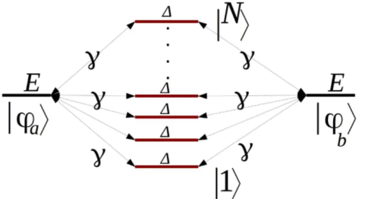
Using the A–N–B canonical basis set |φa〉, |j〉 (j = 1, N)and |φb〉, Fig. 1 is presenting the complete N + 2 quantum states graph of a quantum bus with N 1-state per
trans-fer line interacting with the emitter state |φa〉 and the receiver state |φb〉. Each 1-state line is γ interacting equally
with |φa〉 and |φb〉 and there is a non zero energy difference Δ between the quantum bus states |φa〉 and |φb〉. This
defines two quantum γ, Δ and one classical N control parameters for the A–N–B system.
The quantum properties of the Fig. 1 system have already been studied in detail for the purpose of engineer-ing a bistable switch after playengineer-ing with the electronic couplengineer-ing of one transfer line1. We recall in this section the
essential characteristics of this system not for switching but to focus on another aspect of its quantum contro-lability: the speed up of the electron transfer between A and B as a function of N. On its canonical basis set, the mono-electronic Hamiltonian of the Fig. 1 system is given by1:
Figure 1. The quantum graph of an N 1-state per line bus interconnecting A and B with |φa〉 for the
electron on A, |φb〉 the electron on B and |j〉 for the electron on the bus states. This determines the valence
bond like canonical basis set of the system. The N parallel states have the same electronic energy Δ relative to |φa〉 and |φb〉 and are interacting with |φa〉 and |φb〉 via the electronic coupling γ.
www.nature.com/scientificreports/
γ γ γ γ γ γ γ γ γ γ γ γ γ ∆ = ∆ ∆ ∆ . H N( , , ) 0 0 0 0 0 0 0 0 0 0 0 0 (1)Its spectrum has N + 2 eigenvalues, N − 1 degenerated of value Δ and one λ3 = 0. The two remaining ones λ1 and
λ2 are given by:
λ = 1 ∆ ± ∆ + Nγ
2[ 8 ] (2)
1,2 2 2
For γ∆, only two of those eigenvalues have their corresponding eigenvector very close to |φa〉 and |φb〉. In this
case, the effective through bus coupling Vab(N) is simply 1/2 the energy splitting between λ2 and λ3 leading to
γ
∆
V Nab( ) N
2
which is increasing linearly with N. For γ > Δ or for Δ = 0, the search for those two eigenvectors in the H(N, Δ, γ) spectrum is more difficult that in the previous case. For example for Δ = 0, the λ3 corresponding
eigenvector has still the highest weight on |φa〉 and |φb〉. But at the same time, λ1 and λ2 have exactly the same
weight. In the intermediate regime where γ and Δ are of the same order of magnitude, λ2 is still the second lead-ing one and V Nab( )=(λ2−λ3)/2= 14[∆ − ∆ +2 8Nγ2] i.e. an N law for Vab(N).
Following protocol (ii), one way to determine Vab(N) for all the γ and Δ cases is to prepare the Fig. 1 system at
t = 0 in the non-stationary state |φa〉 to trigger a spontaneous response of the complete A–N–B system in time and
to determine the effective Ωab(N) oscillation frequency of the transfer process. As compared to the above spectral
analysis for tracking Vab(N), the advantage of this preparation is that |φa〉 is now specified and therefore by
sym-metry |φb〉. After this preparation, the time response is given by the solution of the i ∂∂t −H N( , , )∆ γ Ψ( )t =0
time dependent Schrödinger Equation leading after a projection on the canonical basis set used in Fig. 1 to the 3 coupled equations: γ γ γ γ = ∆ . i C t C t C t N N N N C t C t C t ( ) ( ) ( ) 0 0 0 0 ( ) ( ) ( ) (3) a b a b
This system was obtained after calculating the |Ψ(t)〉, Ca(t), Cb(t), C1(t), …CN(t) coordinates on the canonical
basis set, after taking into account the symmetry of the A–N–B system i.e. C1(t) = C2(t) = … = CN(t) = C(t) and
finally after performing the transformation C t( )= NC t( ) as implemented in ref. 2. After solving (3) analyti-cally, the variation in time of the |φb〉 population amplitude is given by:
∑
γ = λ = C t( ) N A e , (4) b m m i t 2 1 3 / mwhere Am = ∏2k m≠ (λm−λk)−1 with λi for i = 1, 2, 3 the eigenvalues of 3. The population of the target state |φb〉
is given by:
∑
γ λ λ = − = C t( ) N A A cos t (5) b i j i j i j 2 2 4 , 1 3 This almost periodic function leads to resonant and anti-resonant time dependent evolutions for well defined
γ and Δ values. For Δ = 0, |Cb(t)|2 is always periodic for all N. For Δ ≠ 0 such a resonant regime is reached only
when γΔ−1 takes the values1:
γ∆ = − − − − N p p m 1 8 2 1 1 , (6) 1 1/2 2 1/2
for integer p and m, and for p m⩾ +1 and p ≠ 2m + 1. As a consequence and whatever γΔ−1, a 1-state per line
bus always permits to reach |φb〉 from |φa〉 in time with no attenuation in average of the |Cb(t)|2 maximum
ampli-tude over time as a function of N.
Since there is one zero eigenvalue for the reduced Hamiltonian (3), Cb(t) is the sum of two power 2 sinusoidals
of frequency
λ1 and λ2
. This is a generic property of a quantum bus with an odd number of states per line. Then,
the Ωab(N) effective oscillation frequency between |φb〉 and |φa〉 is given by the largest component in (5). For non zero
γ and Δ, the largest component is A3A1 and the secular frequency is given by:
γ Ω ( )N = − ∆ + ∆ + N . 2 1 2 8 (7) ab 2 2
According to (7) and for γ∆, Ωab( )N =2∆γ N
2
is linearly dependent on N as already demonstrated in the
spectral analysis above. For γ∆, Ωab(N) is following a N moderate increase with N. For resonant Δ = 0,
Ωab( )N = γ 2N because here the eigenvalues of the 2 eigenstates involved in the transfer process are
λ = ±1,2 γ 2N. Those 3 last cases were not accessible in the above spectral analysis and are leading to an
effec-tive Vab(N) proportional to N.
N transfer lines in parallel with 2-states per line.
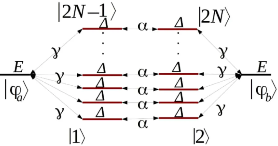
Using the A–N–B canonical basis set |φa〉, |j〉 (j = 1, …,2N) and |φb〉, Fig. 2 is presenting the complete 2N + 2 quantum states graph of the second quantum bus
consid-ered in this work with N 2-state per transfer lines interacting with the emitter state |φa〉 and the receiver state
|φb〉. Each 2-states line is γ interacting equally with |φa〉 and |φb〉 and there is also a non zero energy difference
Δ between the quantum bus states and |φa〉, |φb〉. This defines three quantum α, γ, Δ and one classical N control
parameters for this second A–N–B system.
On its canonical basis, the mono-electronic Hamiltonian of the Fig. (2) system reads:
α γ γ γ γ γ γ γ γ α γ α γ α γ α γ α γ α ∆ = ∆ ∆ ∆ ∆ ∆ ∆ H( , , , )N 0 0 0 0 0 0 0 0 0 0 0 0 0 0 0 0 0 0 0 0 0 0 0 0 0 0 0 0 0 0 0 0 0 0 0 0 0 0 0 0 (8)
Its spectrum has 2N + 2 eigenvalues, N − 1 are degenerated of value Δ − α, N − 1 degenerated of value Δ + α and the 4 last ones are given by:
λ = ∆ −α± (∆ −α) +4Nγ λ = ∆ +α± ∆ +α + Nγ . 2 , ( ) 4 2 (9) 1,2 2 2 3,4 2 2
For γ∆, two cases are observed. For α γ⩽ , two of those eigenvalues, λ2 and λ4, have their corresponding
eigen-vector very close to |φa〉 and |φb〉. This leads to V Nab( ) ∆ −∆Nγα
2
2 2, which is increasing linearly with N as for a 1-state per
line bus case. For α > γ, the two concerned eigenstates are now the ones with their respective eigenvalues λ4 and λ1
leading to α ∆ + + γ α ∆ ∆ − V Nab( ) 21 N 2
2 2 also linearly depending on N. For γ∆ down to γ = Δ, two cases are also
observed. For α γ⩽ , V Nab( )=(λ2−λ4)/2= − −α2 41[ (∆ −α)2+4Nγ2 − (∆ +α)2+4Nγ2]. For
α > γ, the two eigenvalues corresponding with their respective eigenvectors closed to |φa〉 and |φb〉 are now λ1 and λ4
leading to V Nab( )=(λ1−λ4)/2= − +2α 41[ (∆ −α)2+4Nγ2 + (∆ +α)2+4Nγ2] leading finally to an
N law for Vab(N). This is also obtained for Δ = 0 leading to V Nab( )=(λ1−λ4)/2= − +α2 21 α2+4Nγ2.
Finally, there are cases where this spectral analysis does not allow to determine the effective coupling Vab(N). For
exam-ple, when α = γ = Δ, the λ4 eigenvector has still the highest weight on |φa〉 and |φa〉. But at the same time, λ1 and λ2 have
exactly the same weight, which makes the selection of only two eigenstates difficult in this case.
Figure 2. The quantum graph of the N 2-states per line bus interconnecting A and B with |φa〉 for the
electron on A, |φb〉 the electron on B and the 2N |j〉 states for the electron on a given state on the bus. Those
2N states of the bus have the same electronic energy Δ relative to |φa〉 and |φb〉. They are interacting with |φa〉
www.nature.com/scientificreports/
Following protocol (ii), Ωab(N) and therefore Vab(N) can be determined in all cases by preparing the Fig. 2
system at t = 0 in the non stationary state |φa〉 triggering a spontaneous response of the complete A–N–B system
in time. As compared to the spectral determination of Vab(N), the advantage of this preparation is here again that
|φa〉 is now specified and therefore |φb〉 by symmetry. After this preparation, the time response is given by the
solution of the γ
− ∆ Ψ =
∂ ∂
i t H N( , , ) ( )t 0 time dependent Schrödinger Equation leading after a projection on the canonical basis set used in Fig. 2 to the 4 coupled equations:
γ γ γ α γ α = ∆ ∆ . − − i C t C t C t C t N N N N C t C t C t C t ( ) ( ) ( ) ( ) 0 0 0 0 0 0 0 0 ( ) ( ) ( ) ( ) (10) a b N N a b N N 2 1 2 2 1 2
Following the section 2.1 approach, this system was obtained after calculating the |Ψ(t)〉. Ca(t), Cb(t), C1(t), …,
C2N(t) coordinates on the canonical basis set, after taking into account the symmetry of the A–N–B system i.e.
C1(t) = C3(t) = …C2N−1(t), C2(t) = C4(t) = …C2N(t) and finally after performing the transformation
=
− −
C2N 1 NC2N 1 and C2N= NC2N. After solving (10) analytically, the variation in time of the |φb〉
popula-tion amplitude is given for this quantum bus by:
∑
αγ = λ = C t( ) N B e (11) b m m i t 2 1 4 / m where B = ∏ ≠ (λ −λ)−m k m3 m k 1. The population of the target state is then simply given by
∑
α γ λ λ = − = C t( ) N B B cos t (12) b i j i j i j 2 2 2 4 , 1 4Contrary to the 1-state per line case, the maximum |Cb(t)|2 population over time in not unity for all the N
values. But as compared to (6), there is no analytical determination possible of the resonant and anti-resonant
α, γ and Δ values as a function of N. We have not pushed further this analysis to concentrate on the dominant Heisenberg-Rabi oscillation frequency of the quantum oscillation process through this 2-states per line bus.
Since there is no zero eigenvalue for the reduced Hamiltonian (10) and since its spectrum is symmetric, Cb(t)
is the sum of 4 simple sinusoidal terms. This is a generic property of quantum bus with an even number of states per line. As a consequence, there are six different oscillation frequencies in (12): Ωij = (λi − λj)/ħ for i, = j 1 4
with i ≠ j weighted by BiBj.
For α < Δ, the largest coefficient in (12) is B2B4 with the corresponding Heisenberg-Rabi oscillation frequency
Ωab(N) = Ω24 given by: α α γ α γ Ω ( )N = − − 1 ∆ − + N + ∆ + + N 2 ( ) 4 ( ) 4 , (13) ab 2 2 2 2 leading for ∆γ to Ω α γ α ∆ − N ( ) ab (2 N ) 2 2 2
which is linearly dependent on N. But for ∆γ or Δ = γ, Ωab(N) is
following a N moderate increase with N.
For α > Δ, the largest coefficent in (12) is now B1B4 with the corresponding Heisenberg-Rabi oscillation
fre-quency Ωab(N) = Ω14 given by:
α α γ α γ
Ω ( )N = − + 1 ∆ − + N + ∆ + + N
2 [ ( ) 4 ( ) 4 ] (14)
ab 2 2 2 2
leading also for ∆γ to Ω α γ α ∆ − N ( ) ab (2N ) 2 2 2
which is linearly dependent on N. For ∆γ or Δ = γ, Ωab(N) is
again following a N law. Notice that the variation of Ωab(N) as a function of α is not a continuous function with
an effective frequency jump for α = Δ. This explains the above change of the largest coefficient in (12) between
B2B4 and B1B4.
For the resonant case Δ = 0, the largest coefficient in (12) is also B1B4 leading to the corresponding Ωab(N):
α α γ
Ωab( )N = Ω = −14 + 1 2+4N 2 (15)
which is linearly dependant on N for αγ and is following a N law for α ≤ γ.
Finally and in the very peculiar case α = γ = Δ, the two coefficients B1B4 and B2B4 in (12) are equal. This
makes the analytical calculation of the corresponding Heisenberg-Rabi oscillation frequency very cumbersome and for N 1, the Heisenberg-Rabi frequency becomes Ωab( )N = γ21N.
Discussion
The above detail analysis was necessary to appreciate the richness of the time dependant quantum behaviour of 1-state and 2-states per line quantum bus. For γ∆ and for the 2 types of bus, Ωab(N) and therefore Vab(N) is
When γ ≥ Δ or when Δ = 0, the spectral analysis (i) is not able to capture the richness of the quantum mixing between |φa〉, |φb〉 and all the other states of the canonical basis set. In this case, the interest of preparing a non
stationary initial state like |φa〉 is to ease for the determination of Vab(N) via Ωab(N) when the control parameters
are not permitting a clear spectral identification of the eigenstate participating the most in the construction of |φa〉 and of |φb〉 by symmetry. Starting from |φa〉, the determination of the Heisenberg-Rabi secular oscillation
frequency is a good way to pick up over time the two pertinent eigenstates. By practicing this protocol (ii) prepa-ration, the Ωab(N) variations with N are generally showing a N variation which is not the intuitive superposition
law mentioned in the introduction.
Measuring Ω
ab(N) using a tunnel junction
Following now protocol (iii), the measurement of Vab(N) using Ωab(N) requires that A and B interact
electroni-cally with two metallic nano-pads MA and MB respectively using states |φa〉 and |φb〉 as the two pointer states of
the electron transfer process from MA to MB through A–N–B. With no bias voltage applied to the MA-A-N-B-MB
junction, MA will sometime and randomly transfer one electron to A (or MB to B). In this case, no potential
dif-ferent results between MA and MB and the required A–N–B elementary charging energy is coming from thermal
fluctuations since MA and MB are necessarily in interactions with some thermal reservoirs, for example the surface
supporting the MA-A-N-B-MB junction15. When a low bias voltage difference V is applied between MA and MB, a
net current flows through the junction and its intensity I(N) is given by the Landauer formula16:
= I N e h T E N V ( ) 2 ( , )f (16) 2 where e h
22 is the quantum of conductance.
Averaged in time, I(N) results from a large number of electrons transferred events per second occurring from
MA to MA through A–N–B15. From A to B through the quantum bus, each individual electron transfer event is
described by an Heisenberg-Rabi time dependent quantum oscillations as discussed in section 2. At low bias volt-age, we model the quantum measurement at work on this process and performed by the MA-A-N-B-MB junction
by the transformation:
∫
µ= ∞
T E N( , )f 0 C t db( ) h( , )E tf (17)
2
where Cb(t) is the population amplitude of state |φb〉 defined in section 2 for the two types of bus. With (17), the
intrinsic quantum time evolution running in the junction is not eliminated but filtered and transduced to give rise to T(Ef, N). For a low electronic coupling between |φa〉 and |φb〉 through the bus, different μh(Ef, t) transduction
functions have already been proposed in the past and even a μh(E, t) for large V. It is generally a time dependent
damping exponential to avoid the divergence when calculating (17)17–19 or to reproduce the low pass filtering
effect of a tunnel junction20. This is also what was anticipated by Lipmann and Schwinger21 to eliminate the fast
time variations near and on the scattering center from their model of quantum scattering and to be able to work only with asymptotic states far away from this scattering center.
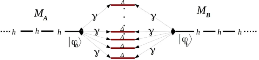
To determine μh(Ef, t), we have applied (17) to the Fig. 1 A–N–B system. Here, each line of this 1-state per line
bus is now interacting with 2 semi-infinite chains to model the MA and MB nano pads, each with a single
conduc-tion band and a 4 h bandwidth as presented in Fig. 3. For simplicity, |φa〉 and |φb〉 are supposed to have the same
energy than the on-site energy of an electron propagating site by site along the MA or the MB chains. Cb(t) and
T(Ef, N) can be both calculated analytically with Cb(t) given by (4) and T(Ef, N) given in ref. 1:
γ γ = + ∆ . T E N N N h ( , ) 4 4 (18) f 2 4 2 4 2 2
After some calculations to obtain (18) from (17) and after the introduction of (4) in (17), the μh(Ef, t)
meas-urement function reads:
Figure 3. The schematic model of two semi-infinite quantum chains to model the MA and MA nano-pads
interacting with the simple Fig. 1 A–N–B quantum system. h is the interstate coupling along those chains and Δ is the energy difference between those chains states and the central A–N–B system.
www.nature.com/scientificreports/
µ = = − . ∆ ∆ −(
∆ − ∆ −∆)
E t h ( 0, ) 2 / 1 e (19) h f ih i i h t , 4 2 4 / 2 At Ef, (19) can in fact be applied to any quantum system introduced in the tunnel junction if it is interacting with
the nano-pads only via the pointer states |φa〉 and |φb〉. In particular when there are no quantum states in the
junction, a small Ω through space electronic coupling can remain between MA and MB. This is exactly the
condi-tions used by J. Bardeen9 to get the low bias voltage V tunneling current intensity I∝ Ω ρ ρ V
M M
2
A B through a
simple MA–Ω–MB tunneling junction where ρM
A and ρMB are the MA and MB electronic density of states. For the
simple Fig. 3 MA and MB conducting chains ρM =ρM = 4π1h
A B leading to: ∝ Ω I h V (20) 2 2
For this simple case, the corresponding μh(Ef, t) measurement function is given for Ef = 0 by:
µ = − .
d h( )t 2 / eh ht/dt (21)
In this case and disconnecting now the two MA and MB measurement chains to return to the measurement
protocol (ii), it remains a 2 states isolated quantum system |φa〉 and |φb〉 with a through space electronic coupling
Ω between them. As described in section 2 and preparing this simple system in the non-stationary state |φa〉,
the time variations of the |φb〉 population amplitude during the Heisenberg-Rabi oscillation process is simply
Cb(t) = sin Ωt/ħ. Then, using (20) and inserting this Cb(t) in (17) leads to:
= Ω + Ω . T E h h ( ) 4 ( ) (22) f 2 2 2 2 2 2 2
which is the exact T(Ef) one can calculate analytically applying a simple scattering approach on a valence bond
like canonical mono-electronic basis set22. Interestingly, (22) reduces to (20) for Ω h confirming that at low
coupling and for this very simple MA–Ω–MB quantum system T(Ef) is proportional to the square of the Cb(t)
oscillation frequency15. This indicates that μ
h(Ef, t) is rather universal. Its extension for the complete energy range
of the MA and MB measurement bandwidth is now under exploration.
As exemplified with (16) and also for the simple MA–Ω–MB Bardeen tunnel junction, (17) with (19) is able to
pick up at low coupling the secular oscillation frequency of Cb(t) leading to T(Ef, N) ∝ Ωab(N)2. There is a limit
for the functionning of this transduction because T(Ef, N) is bond from above to unity and as demonstrated in
section 2, Vab(N) and then Ωab(N) are monotonically increasing with N. This limit manifests itself by the peculiar
variation of T(Ef, N) as a function of Ωab(N) when Ωab(N) is increasing so much that T(Ef, N) is saturating to unity.
According to (4) and (14), Cb(t) is a linear superposition of sinusoidal terms with different oscillation
frequen-cies. To understand the functioning of (17) and since under its modulus, (17) is a linear transformation, one can choose for Cb(t) simply a sin(Ωt/ħ) or a sin2(Ωt/ħ) depending respectively of the odd or even number of state in
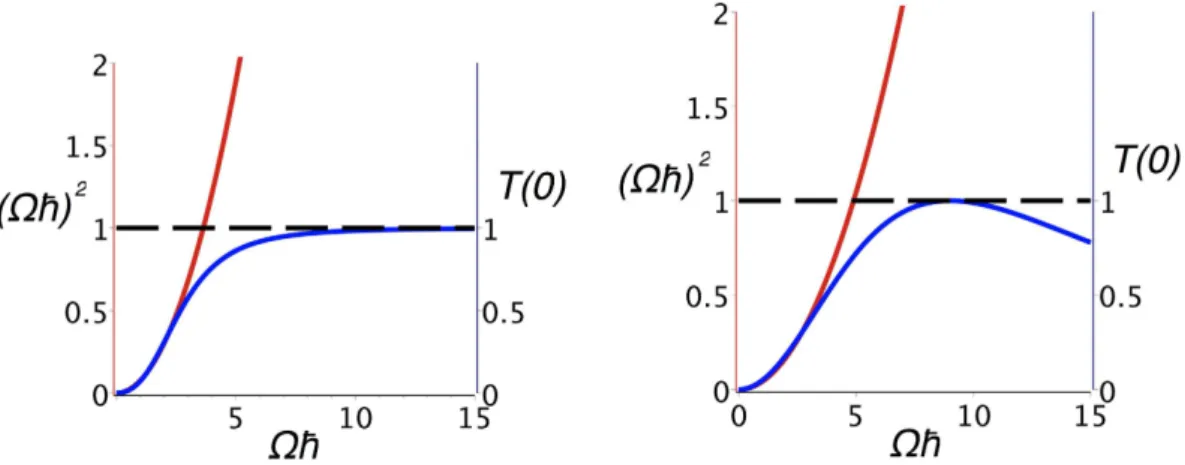
the bus lines. The unique property of (17) is that for Cb(t) = sin(Ωt/ħ), T(Ef) will decrease for large Ω after
reach-ing T(Ef) = 1 while for Cb(t) = sin2(Ωt/ħ), T(Ef) will simply saturate to unity for large Ω (Fig. 4). This behaviour
is at the origin of the debate in the literature about the validity of the I(N) = N2. J superposition law refs 1 and 12.
The second property of (17) is its low pass filtering character on any Cb(t) due to the μh(Ef, t) exponential time
dependant term. As already noticed in ref. 20, this implies that the large Cb(t) frequency components will not be
capture in T(Ef) because for Ω > h/ħ, T(Ef) is first saturating to unity. Therefore, (17) permits the determination of
the secular Cb(t) oscillation frequency using in (17) a well tuned μh(Ef, t) function that is with a good selection of
the electronic bandwidth of the MA and MB nano-electrodes around Ef.
The parallel quantum circuit law
Knowing the general properties of the linear transformation (17) to pass from Cb(t) to its corresponding T(Ef), we
can now discuss how the richness of the time dependent quantum behaviours of 1-state and 2-states per line bus discussed in section 2 are preserved or not through the (17) transduction effect corresponding to protocol (iii). For a 1-state per line bus, starting from (4) and using (17), the T(Ef, N) analytical expression is given by:
γ γ = + ∆ . T E N N N h ( , ) 4 4 (23) f 1 2 4 2 4 2 2
and for a 2-states per line bus using now (14) in (17):
γ α γ α γ α = + ∆ − + . T E N N h N h N h ( , ) 4 [ ( ) ] 4 (24) f 2 2 4 2 2 2 4 2 2 2 2 2 4 2 2
Both expressions can also be directly obtained using the Elastic Scattering Quantum Chemistry (ESQC) method starting from a mono-electronic Hamiltonian and calculating directly the corresponding scattering matrix22. By doing so, the time dependent Heisenberg-Rabi oscillations are not showing up explicitly since such
electrodes. This is not a problem for γ∆ because in this case Ωab(N) and therefore Vab(N) are not large enough
to saturate (17) to unity assuming that N is small enough not to compensate for this small coupling through the bus. This becomes a problem for non tunneling regime or when the number N of lines in the bus is compensating for the initial low coupling through a single line. In this case, there is generally no more relation between T(Ef, N)
and the increasing Ωab(N) as a function of N. In effect, for γ∆ and for moderate N values, (23) and (24) are
leading to a N2 variations for both T(E
f, N)1 and T(Ef, N)2 as a function of N up to the point where the increase in N
is compensating for the initial small γ value. In this case, the N2 law is no more valid with a saturation of T(E
f, N)1
whatever N and a decreasing of T(Ef, N)2 for large N after its saturation to unity.
In Fig. (5), the range of the N2 law validity is presented by plotting the
= T E N T E N ( , ) ( , 1) f f 2 2
ratio for a 2-states per line bus. For small γ (Fig. 5 right panel), the N2 law is valid at least for N going from 1 to 5. But for large γ, this is no
more the case. As discussed in section 3 and illustrated in Fig. 4, this is caused by the property of the transforma-tion (17). Notice that this N2 law is valid for any odd and even number of states per line in the bus as soon as the
increase in N is not compensating the γ∆ tunneling condition. Notice that for γ∆, this N2 superposition
law is a generalisation for the case of N quantum conductance connected in parallel of the =G G1+G2+2 G G1 2
superposition law known in a tunnel regime for 2 quantum conductances G1 and G2 connected in parallel via a
quantum node11 since for this peculiar N = 2 case, it comes G = 4g for G
1 = G2 = g.
More interesting are now the cases where γ is closed or larger than Δ or when Δ = 0. Here, the value of h rel-ative to Δ must also be considered because h is determining the energy range of the (17) transduction function. Furthermore and according to (23) and (24), h is playing the same role than α, γ and Δ in controlling this trans-duction. In this case and as discussed in section 2, there are many quantum control parameters values where Ωab(N) is only proportional to N.
Figure 4. Illustration of the transduction process saturation at work in a tunneling junction. Cb(t) in (17) is
here simulated by sin(Ωt/ħ) for an odd number of state per line case (left) and by sin2(Ωt/ħ) for an even number
of states per line (right). In both cases, the red curve is indicating the Ω2 variation expected at low coupling for
T(Ef). Due to the T(Ef) normalisation to unity and also to the low pass filter character of the μh(Ef, t)
transduction function in (17), T(Ef) is either saturating (left) or even decaying (right) when Ω is increasing
indicating the quantum limitation of this transduction process which can be tuned by changing the value of h in
μh(Eh, t).
Figure 5. The ratio between T(Ef, N)2 and T(Ef, N = 1)2 for a bus with N 2-states transfer lines mounted in
parallel for Δ = 0.0 eV (left) and Δ = 10.0 eV (right) with h = 4.0 eV and = N 1 5 calculated at Fermi energy.
www.nature.com/scientificreports/
The case raised up by C. Lambert and co-workers and underlined in the introduction is corresponding exactly to N = 2 for a 2-states per line bus with Δ = 0 and α = γ = h12. For this case, section 2.2 is giving
Ωab( )N = γ1+ 44NN+1 which is following a N increase with N. But using now (24) for this C. Lambert case, =
+
( )
T E N( , )f 2 N2N1
2
2 leading for N = 2 to T E N( , )f 2= 1625. There is here a notable decrease in electronic
trans-parency in passing from N = 1 to N = 2 since for N = 1, T(Ef, N)2 = 1. This clarifies the literature debate
concern-ing the N2 power law. It turns out that the case raised up in ref. 12 is not a tunneling case. Already for N = 2 and
since Δ = 0 and α = γ = h, T(Ef, N)2 is already in its decaying regime for an N increase due to the properties of the
transduction function (17).
To push further the discussion using (23) and (24), it is important to notice that for a 1-state per line bus, N2 is
appearing both at the numerator and the denominator of (23). Therefore and after a T(Ef, N)1 saturation to unity
for large N, it is impossible to follow the richness of any quantum behaviour observed in section 2 using the trans-duction (17). This is for example the case of the N variations of Ωab(N) for large N. For a 2-states per line bus and
aside from the C. Lambert case Δ = 0, there are many interesting Heisenberg-Rabi time-dependent quantum behaviours which can be capture by (24) since now there is an N4 term in the T(E
f, N)2 denominator and only an
N2 in its numerator. In (24), the (Δ2 − α2) term is also playing a important role. For example for the case
α = Δ = h = γ i.e. where according to section 2.2, Ωab( )N = γ21N, the decreasing of Ωab(N) with a N increase is
well captured by (17) leading to T E N( , )f 2= 1 ( / 2)+ N1 2. This indicates how important is the h tuning to follow the
Ωab(N) variations with N i.e. to optimize the transduction process at work in a tunnel junction.
Conclusions
We have started by analysing the quantum spectral properties of 1-state per line and 2-states per line bus with the objective to determine how the Vab(N) effective electronic coupling through such bus between an emitter and a
receiver states varied as a function of the number N of lines connected in parallel to form this bus. For cases where it was spectrally difficult to determine Vab(N), we have re-enforced this analysis by triggering an Heisenberg-Rabi
time dependent through bus quantum exchange process with an effective secular oscillation frequency Ωab(N).
For this purpose, we have prepared a specific initial non-stationary pointer state and used its symmetric target pointer state to determine Ωab(N). This leads to two different Ωab(N) (and therefore Vab(N)) regimes of variations
as a function of N: a linear one following the intuitive superposition of electronic couplings and a N moderate increase as a function of N. In a way to substitute the initial pointer state preparation by electronically coupling the quantum bus with semi-infinite electrodes, we have discussed how the quantum transduction measurement process at work in such a tunneling junction can or not faithfully follow the variation with N of the through bus
Vab(N) effective electronic coupling. Due to the normalisation to unity of the electronic transparency of any
quan-tum bus and to the low pass filter like character of the transduction process at work in a tunnel junction, large
Vab(N) increase due to an N increase cannot be detected by a tunneling junction. The N2 superposition law is
preserved for Ωab(N) (and therefore Vab(N)) for low coupling as soon as N is small enough not to compensate for
this small through bus coupling per line. The limitations of the quantum transduction at work in a tunneling junction is also pointing out how the broadly used concept of electrical contact between a metallic nanopad and a molecular wire may be better described in term of a quantum transduction process. This is opening the way for a better optimisation of this transduction process at work in a tunneling junction for example by engineering the electronic band structure of the conducting nanopads in charge of this transduction to optimize the so-called contact conductance.
References
1. Joachim, C. Control of the quantum path-target state distance: bistable-like characteristic in a small tight-binding system. J. Physics
A: Mathematical and General L1149, 20 (1987).
2. Chen, B. et al. Multipath adiabatic quantum state transfer. Phys. Rev. A. 88, 022323 (2013).
3. Launay, Jean-Pierre. Long-distance intervalence electron transfer. Chem. Soc. Rev. 30, 386–397 (2001).
4. Nakamura, Y., Pashkin, Y. A. & Tsai, J. S. Coherent control of macroscopic quantum states in a single-Cooper-pair box. Nature 398, 786–788 (1999).
5. Tan, S. F. et al. Quantum plasmon resonances controlled by molecular tunnel junctions. Science 343, 1496–1499 (2014).
6. Joachim, C. Ligand-length dependence of the intramolecular electron transfer through-bond coupling parameter. Chem. Phys. 116, 339 (1987).
7. Felker, P. M. & Zewail, A. H. Dynamics of intramolecular vibrational-energy redistribution (IVR). II. Excess energy dependence. J.
Chem. Phys. 82, 2975 (1985).
8. Sautet, P. & Joachim, C. The switching ability of a three-level tight-binding system: the isolated and embedded case. Journal of
Physics C: Solid State Physics 21, 3939–3957 (1988).
9. Bardeen, J. Tunnelling from a Many-Particle Point of View. Phys. Rev. Lett. 6, 57 (1961).
10. Joachim, C. Molecular electronics: Probing intramolecular circuit laws. Nature Nano. 7, 620 (2012).
11. Magoga, M. & Joachim, C. Conductance of molecular wires connected or bonded in parallel. Phys. Rev. B. 59, 16011 (1999). 12. Sadeghi, H. et al. Conductance enlargement in picoscale electroburnt graphene nanojunctions. PNAS. 112(9), 2658–2663 (2015). 13. Vazquez, H. et al. Probing the conductance superposition law in single-molecule circuits with parallel paths. Nature Nanotechnology
7, 663–667 (2012)
14. Lang, N. D. & Avouris, P. Oscillatory Conductance of Carbon-Atom Wires. Phys. Rev. Lett. 81, 3515 (1998).
15. Joachim, C. & Ratner, M. A. Molecular electronics: Some views on transport junctions and beyond. PNAS 102, 8801 (2005). 16. Büttiker, M., Imry, Y., Landauer, R. & Pinhas, S. Generalized many-channel conductance formula with application to small rings.
Phys. Rev. B. 31, 6207 (1985)
17. Ness, H. & Fisher, A. Nonperturbative evaluation of STM tunneling probabilities from ab initio calculations. Phys. Rev. B. 56, 12469 (1997).
18. Sanchez, C., Stamenova, M., Sanvito, S., Bowler, D. R., Horsfield, A. P. & Todorov, T. N. Molecular conduction: do time-dependent simulations tell you more than the Landauer approach? J. Chem. Phys. 124, 214708 (2006).
The authors like to thank the PAMS integrated FET european project for financial support during this work.
Author Contributions
C.J. designed the research project. O.F.N. and G.D. performed the demonstration and computer simulations. C.J. and O.F.N. provided the interpretations. O.F.N. and C.J. wrote the manuscript. All authors reviewed the manuscript.
Additional Information
Competing financial interests: The authors declare no competing financial interests.
How to cite this article: Namarvar, O. F. et al. Parallel Quantum Circuit in a Tunnel Junction. Sci. Rep. 6, 30198; doi: 10.1038/srep30198 (2016).
This work is licensed under a Creative Commons Attribution 4.0 International License. The images or other third party material in this article are included in the article’s Creative Commons license, unless indicated otherwise in the credit line; if the material is not included under the Creative Commons license, users will need to obtain permission from the license holder to reproduce the material. To view a copy of this license, visit http://creativecommons.org/licenses/by/4.0/