β-delayed charged particle decays of neutron-deficient nuclei $^{20}$Mg and $^{22.23}$Si

HAL Id: tel-01461303

http://hal.in2p3.fr/tel-01461303

HAL is a multi-disciplinary open access

archive for the deposit and dissemination of sci-entific research documents, whether they are pub-lished or not. The documents may come from teaching and research institutions in France or abroad, or from public or private research centers.

L’archive ouverte pluridisciplinaire HAL, est destinée au dépôt et à la diffusion de documents scientifiques de niveau recherche, publiés ou non, émanant des établissements d’enseignement et de recherche français ou étrangers, des laboratoires publics ou privés.

nuclei

Mg and

Si

M. Babo

To cite this version:

M. Babo. β-delayed charged particle decays of neutron-deficient nuclei 20_{Mg and} 22.23_{Si. Nuclear}

! !

THESE

Pour obtenir le diplôme de doctorat

Spécialité

Physique

!

Préparée au sein de l’Université Caen - Normandie

β-delayed charged particle decays of

neutron-deficient nuclei

Mg,

Si and

Si

Présentée et soutenue par

Mathieu BABO

Thèse dirigée par Olivier SORLIN, GANIL

! ! ! !

!

Thèse soutenue publiquement le 16 Septembre 2016 devant le jury composé de

Dr Olivier SORLIN Directeur de Recherche, GANIL, Caen Directeur de thèse Dr Bertram BLANK Directeur de Recherche, CENBG, Gradignan Rapporteur Dr Daniel BAZIN Professeur, NSCL, East Lansing Rapporteur Dr Riccardo RAABE Professeur, KU Leuven, Leuven Examinateur Dr Etienne LIENARD Professeur, Université de Caen / LPC, Caen Examinateur

U.F.R. de Sciences

´

ECOLE DOCTORALE SIMEM

Th`

ese de doctorat

pr´esent´ee et soutenue le : 16 Septembre 2016

par

M. Mathieu Babo

pour obtenir le

DOCTORAT de l’UNIVERSIT´

E de CAEN

Sp´ecialit´e : Constituants ´el´ementaires et physique th´eorique

β-delayed charged particle decays of the

neutron-deficient nuclei

20

Mg,

23

Si and

22

Si.

MEMBRES du JURY :

Dr. Olivier Sorlin Directeur de recherche, GANIL, Caen (Directeur de th`ese) Dr. Bertram Blank Directeur de recherche, CENBG, Gradignan (Rapporteur )

Dr. Daniel Bazin Professeur, NSCL, East Lansing (Rapporteur ) Dr. Riccardo Raabe Professeur, KU Leuven, Leuven

au laboratoire NSCL, `a MSU (USA), puis implant´es dans un dispositif compos´e de 3 d´etecteurs Si `

a pistes (DSSD) entour´e de 16 d´etecteurs HPGe. Cet ensemble a permis la d´etection des particules charg´ees ´emises depuis les ´etats non li´es, en coincidence avec les rayons γ ´emis par la d´esexcitation des noyaux fils. La d´ecroissance βp du 20_{Mg, particuli`erement bien connue, a ´et´e ´etudi´ee afin de tester et}

d’optimiser l’analyse. En particulier, les voies de d´ecroissance βp peuplant les 3 premiers ´etats excit´es du

19

Ne ont pu ˆetre identifi´ees. Le temps de demi-vie, les rapports d’embranchement des transitions et les ´energies d’excitation des ´etats, y compris l’´etat isobarique analogue (IAS), ont ´et´e mesur´es. L’´etude de la d´ecroissance β du23_{Si a permis l’identification de 14 ´etats dans l’}23_{Al. L’´emission de deux protons depuis}

l’IAS dans l’23_{Al a pu ˆetre mise en ´evidence avec certitude. La mesure de l’´energie de l’IAS a permis}

une d´etermination plus pr´ecise de la masse de l’´etat fondamental du23

Si, `a 23.27 (7) MeV. Une possible transition β3p a ´egalement ´et´e observ´ee. La plupart des pr´edictions th´eoriques de la masse du22_{Si sont}

en accord avec une radioactivit´e 2-protons (2p). Les d´ecroissances β2p vers le premier ´etat excit´e et l’´etat fondamental du 20_{Na ont ´et´e identifi´ees. Le rapport d’embranchement vers l’IAS est de 2.05 (44) %, et}

son ´energie d’excitation a ´et´e mesur´ee `a 9040 (54) keV. La mesure suppl´ementaire du temps de demi-vie, T1/2= 30.38 (45) ms, a permis de calculer le temps de vie partiel de cette transition. Dans cette ´etude,

nous proposons une param´etrisation de la fonction statistique de Fermi f pour les d´ecroissances de Fermi super-permises, permettant la premi`ere mesure indirecte de l’exc`es de masse de l’´etat fondamental du

22_{Si, `a 31.49 (14) MeV. L’´energie seuil correspondante est alors S}

2p= 645 (100) keV, et ne permet pas

une radioactivit´e 2p depuis l’´etat fondamental.

Abstract

The neutron-deficient nuclei 20_Mg, 23_{Si and} 22_{Si were produced by fragmentation at NSCL, at MSU}

(USA), and implanted into an array of 3 double sided stripped Si detectors, surrounded by 16 high-purity Ge detectors. This novel arrangement allowed the detection of the charged particles emitted by the unbound excited states in coincidence with the γ rays emitted by the de-excitation of the daughter. The βp decay of20_{Mg is very well-known and therefore was used to test and optimize the analysis programm.}

The β-delayed proton transitions to the first 3 excited states in 19_{Ne were identified and compared to}

previous measurements. The half-life, the branching ratio of the transitions and the excitation energies, including the IAS, were measured and are in good agreement with the adopted values. The study of the β+_{decay of}23_{Si allowed the identification of 14 excited states in}23_{Al. The emission of 2 protons from the}

IAS was unambiguously identified. The measurement of the IAS energy allowed a better determination of the mass excess of 23_{Si, giving 23.27 (7) MeV. A possible β3p decay channel was also tentitavely}

identified. Most of the theoritical predictions are in favor of a 2-proton radioactive22_{Si. The β2p decays}

to the first excited state and the ground state of20_{Na were identified. The branching ratio of the decay to}

the IAS is 2.05 (44) %, and the IAS excitation energy was measured to be 9040 (54) keV. The additional measurement of the half-life gives T1/2 = 30.38 (45) ms, and allowed the determination of the partial

half-life. In this study, we propose a parametrization of the statistical rate function f for the superallowed Fermi β decays. This allow the first indirect mass measurement of 22_{Si ground state, 31.49 (14) MeV.}

1 Introduction 7

1.1 Nuclear β-decay . . . 9

1.1.1 Fermi Theory of β Decay . . . 10

1.1.2 Classification and selection rules . . . 13

1.1.3 The f t value . . . 14

1.1.4 Superallowed Fermi β Decays . . . 16

1.2 β-delayed charged particle decays . . . 18

1.2.1 The Isobaric Mass Multiplet Equation . . . 20

1.2.2 β-delayed multiple charged particle decays . . . 22

1.3 One-Proton and Two-Proton radioactivity . . . 24

1.3.1 Two-proton radioactivity . . . 24

1.3.2 Discovery of Two-Proton Radioactivity . . . 27

1.3.3 Summary and Motivation . . . 31

2 Beam Production and Experimental Setup 35 2.1 Isotope Production . . . 35

2.1.1 Secondary Beam Production . . . 35

2.1.2 The Radio Frequency Fragment Separator . . . 37

2.2 Implantation and Decay Detection Station . . . 41

2.2.1 The Beta Counting System . . . 41

2.2.2 The Segmented Germanium Array . . . 54

2.3 Conclusion . . . 62

3 β-delayed proton decay of 20_{Mg 63} 3.1 20_{Mg: a well known βp emitter . . . 64}

3.2 γ-ray spectra from20_{Mg decay . . . 69}

3.3 γ-ray gated proton spectra . . . 70

3.3.1 Eγ = 275 keV . . . 73

3.3.2 Eγ = 1298 keV . . . 74

3.3.3 Eγ = 238 keV . . . 75

3.5 Relative decay branching ratios . . . 78

3.6 Half-life measurement . . . 82

3.6.1 γ-ray gated decay curves . . . 82

3.6.2 Proton-gated decay curves . . . 85

3.6.3 Ungated decay curve . . . 87

3.6.4 Discussion on the half-life . . . 90

3.7 Conclusion . . . 90

4 β-delayed charged particle decays of 23_{Si 93} 4.1 Previous measurements . . . 94

4.2 Experiment analysis . . . 95

4.2.1 20_{Na contamination . . . 97}

4.3 γ-ray spectrum from 23_{Si decay . . . 103}

4.3.1 βp decay channel in coincidence with γ rays. . . 105

4.3.2 β2p decay channel in coincidence with Eγ = 332 keV . . . 117

4.3.3 β3p decay channel in coincidence with Eγ = 1633 keV . . . 120

4.4 The ungated charged particle spectrum . . . 122

4.5 Discussion on the excitation energies . . . 125

4.6 The IMME for T = 5/2 and the mass of 23_{Si . . . 133}

4.7 Half-life measurement . . . 134

4.7.1 Using γ-ray gates . . . 134

4.7.2 Using proton gates . . . 137

4.7.3 Conclusion on the half-life . . . 139

4.8 Conclusion . . . 139

5 β-delayed charged particle decays of 22_{Si 141} 5.1 Discussion on the particle thresholds . . . 141

5.2 Previous study of22_{Si decay . . . 144}

5.3 Present experiment . . . 145

5.4 γ-ray spectrum from 22_{Si decay . . . 147}

5.5 βp decay channel with γ-ray coincidence . . . 150

5.5.1 γ-ray at E = 880 keV . . . 151

5.5.2 γ-ray at E = 204 keV . . . 151

5.6 β2p decay channel with γ-ray coincidence . . . 154

5.7 Ungated proton spectrum with γ-ray subtraction . . . 156

5.8 Decay level scheme of22_{Si . . . 161}

5.8.1 Discussion on E∗ level = 2181 (44) keV . . . 161

5.9 Half-life measurement of22_{Si . . . 170}

5.9.1 Using proton gates . . . 170

5.9.2 Using γ-ray gates . . . 172

5.9.3 Final result: the half-life of 22_{Si . . . 173}

5.10 Mass excess of 22_{Si ground state . . . 175}

5.10.1 Statistical rate function for T = 3 . . . 175

5.10.2 Mass excess of 22_{Si ground state . . . 185}

5.11 Conclusion . . . 186

6 Conclusion and Future work 189 6.1 Conclusion . . . 190

6.2 Future Work . . . 192

6.2.1 New measurement of20_{Mg decay . . . 192}

6.2.2 Observing the β3p channel in23_{Si . . . 192}

Il est int´eressant de se pencher, une fois l′

´epreuve de la r´edaction du manuscrit touchant `a sa fin, sur l′

enchaˆınement d′

´ev`enements qui me mena en cet instant pr´ecis. Nul n’est besoin de s’attarder sur ces d´etails, mais il convient de remettre dans son contexte la naissance de cette th`ese. Et c’est ainsi que, plutˆot que d′

entamer les remerciements par le cˆot´e hi´erarchique, je vais vous les ´enoncer par ordre chronologique.

Les exp´eriences de physique nucl´eaire ne sont pas sans rappeler ces kits de petit physicien en herbe que l′

on m′

offrait les jours de fˆetes. Les nombreux shifts de nuit qui les accompagnent ressemblent d′

ailleurs fortement `a ces nuits pass´ees dans le jardin familial, `a observer les ´etoiles et les plan`etes, le nez tremblant, et l′

œil appuy´e sur la lunette ou le t´elescope. Ce sont l`a mes premi`eres exp´eriences de physique, d′

astronomie et de chimie, mises en œuvre sous les yeux attentifs et protecteurs de mes parents. C’est ainsi que me vient naturellement l′

envie de les remercier. Maman, Papa, mais aussi mes fr`eres Thomas et Marc, vous avez su me porter et me soutenir malgr´e les durs efforts que cela pouvait parfois repr´esenter. Vous avez d´eclench´e en moi cette puissante envie de d´ecouverte, de compr´ehension du monde qui m′

entoure. Vous l′

avez accompagn´ee, en visitant un observatoire pendant nos vacances, ou mˆeme en parcourant quelques centaines de kilom`etres pour assister `a une ´eclipse. Et au-del`a du physicien, c’est ladulte que je suis devenu qui vous remercie.

Cet attrait pour les sciences me permet d′

effectuer un stage, en MPSI/MP, aupr`es de l′

acc´el´erateur TANDEM `a l′

IPN d′

Orsay. C’est ici que se joue l′

´ev`enement le plus d´eroutant de ma vie, dans le sens o`u il me m`enera, non sans embˆuche et contre toute attente, `a mon doctorat. Je me dois, en me rappelant cette semaine de faisceau qui m′

´etait enti`erement d´edi´ee pour mettre en ´evidence ce qu’´etait la magicit´e d′

un noyau, de remercier Tonton Fadi. Grˆace `a toi, j’ai goˆut´e `a la physique nucl´eaire (et au Coca Cola cherry), et je n’ai pas r´eussi `a m′

en d´efaire. Je te remercie de m′

avoir accompagn´e et de m′

avoir soutenu, dans les moments de doute et de faiblesse, mais aussi dans ceux o`u je n’avais plus assez de batterie. Tu as vu en moi cette ´etincelle de chercheur que je n’avais pas mˆeme souponn´ee. Assez naturellement et sans honte, je peux affirmer que ce doctorat, c’est `a toi que je le dois. A toi et au P`ere Fouettard, qui m′

aura pouss´e au bord de mon ignorance, et qui m′

aura appris ce qu’´etait une raie `a 511 keV. Une drˆole de transition, introuvable dans les tables, et qui me poursuit depuis lors. Il m′

est impossible d′

oublier ces autres chercheurs du groupe Nester ; les incroyables Fa¨ırouz, Nicolas, Iulian, Iolanda, Dominique et Matthieu, qui ont ´egalement apport´e leur pierre `a l′

´edifice. La cons´ecration de toutes ces ann´ees d′

´etudes vient alors que je m′

y attends le moins, avec l′

obtention d′

une bourse de doctorat au GANIL. Pour cette th`ese, je dois remercier Olivier, d′

avoir accept´e de m′

encadrer officiellement. Je ne peux que me reprocher d′

avoir si peu interagi, mais je te remercie pour ton honnˆetet´e lors de la derni`ere ligne droite, qui m′

aura permis de me recadrer. De toute l′

´equipe avec laquelle j’ai travaill´e, je dois aussi remercier Geoffrey-Fathom, qui a su me faire confiance en me confiant ce jeu de donn´ees `a analyser. La tˆache ne fut pas

empˆech davancer.

Il ne serait pas convenable de terminer ces remerciements sans parler de mes acolytes de th`ese : Pierre (avec qui je n’aurai pas pu dormir dans un lit en forme de cœur `a Venise mais avec qui j’ai partag´e une fin de th`ese digne des grandes ´epop´ees grecques), Marine (sans qui mes nerfs auraient lˆach´e depuis belle lurette), Coralie (ma copine bretonne et alcoolique), Quentin (courage p′

tit chat, le prochain c’est toi), Alex et Samantha (thank you so much for your support and your help for this last year), Guillaume (tu ne liras mˆeme pas ma th`ese, mais ton cynisme me manque), Dennis, Benoˆıt, Aldric, Adrien, Simon, Patrick, Hong Liang, Yung Hee, et j′

en oublie sˆurement ...

Ces trois ann´ees de th`ese n’auraient pas pu ˆetre un succ`es sans les interactions avec les autres chercheurs du GANIL (Fran¸cois, Anth´ea, Fanny, Carme, Julien, Beyhan, Emmanuel), de l′

IPN (Marion), du CIMAP (Yannick, Lucas, Arek) de l′

INFN (Barbara, Marco R., Marco S., Alberto), de NSCL (Daniel) et de Cologne (Mickael). J’en oublie sˆurement, mais je dois avouer que le manque de sommeil de la fin de th`ese n’arrange pas ma m´emoire.

Dans une autre sph`ere, celle du priv´ee, j’aimerais remercier plus particuli`erement Xtoulov, pour ces coups de mains gauches et ses phrases qui ne veulent rien dire. Merci aux copains Guillaume, Richard et Julien (eh non, pas de Babo bingo cette fois-ci). Merci `a J´erˆome et Francis, pour cette drˆole de famille. Merci `a Guigui, Juju, C´ecile et la d´eesse Britney. Merci `a Romain, qui m′

a aid´e `a accoucher de ce beau b´eb´e qu’est Pint of Science `a Caen. Merci aux femmes du GANIL : Myriam, Ketel, Sabrina, Virginie, Marie-Laure, Catherine, et toutes les autres.

En dernier lieu, il est de mon devoir de vous remercier, vous qui ouvrez ces quelques pages, et qui prenez le temps de parcourir mon travail accompli ces trois derni`eres ann´ees. J’ai bon espoir qu’il vous soit utile, qu’il vous inspire et qu’il vous invite `a le d´epasser.

Introduction

One of the simplest ways to describe the mass of atomic nuclei is to ignore the fact that the nucleus consists of protons, neutrons and the complex N-body forces acting between them and to instead assume that the entire system can be treated as a charged liquid drop. A semi-empirical description would require both volume and surface terms as well as a uniform Coulomb contribution that is required to describe the overall electric charge. By adding additional terms for pairing and symmetry effects, the binding energy of this liquid drop is described by the well-known Bethe-Weizsacker mass equation [Wei35]. The predictive power of this formula is shown in Figure 1.1. It is immediately apparent that this description works reasonably well for most nuclei with the exception of a select few that have a very specific number of protons and/or neutrons. These numbers were deemed magic numbers since they seemed to provide excess nuclear binding.

Today, the concept of magic numbers is well understood. They originate from the fact that nuclei exhibit shell structure in a completely analogous way to electron shell structure in atoms. The nuclear shell model was developed [May48] to explain why these magic nuclei, with proton or neutron numbers equivalent to 2, 8, 20, 28, 50, 82, or 126, are the most strongly bound and why doubly magic nuclei (nuclei with a magic number of both protons and neutrons) provide the strongest possible nuclear configuration. Although tremendously successful, it was assumed that the nuclear shell model with its fixed set of magic numbers is universal and should persist even in unstable isotopes. Following decades of research and with the recent advent of rare-isotope beam facilities, this simple picture is now known to be incorrect. The classical shell gaps and magic numbers used to describe nuclei near stability evolve towards the extremes of nuclear binding and often give rise to spectacular phenomena such as exotic structures, unique shapes, and rare modes of nuclear decay. The delicate and subtle forces that drive these dramatic structural changes challenge our understanding and demand further investigation in regions where they may be enhanced. Experimental studies of nuclear structure and decay for the most exotic nuclei are thus essential for understanding the limits of nuclear binding

Figure 1.1 –Differences between the mass measurements and the predictions of the Bethe-Weizs¨acker formula, as a function of the proton and neutron number. For discrete numbers of nucleons, the differences suddenly increase and translate more stable nuclear configurations. (Figure taken from [Hey04])

and for improving theoretical predictions in areas of the nuclear chart that cannot be accessed experimentally. The primary focus of this thesis is the study of the β decays of the neutron-deficient nuclei 22,23_{Si and} 20_{Mg that are located at the limits of nuclear stability. For these}

nuclei, the energy available for β decay is significant and this energy (or Q value) opens new decay channels. The parent can decay to excited states above the particle separation threshold and these β-delayed particle decays are a powerful spectroscopic tool to study the structure of unbound excited states in weakly-bound nuclei. On the proton rich side of the nuclear chart, where the Coulomb force is less repulsive in the β+ _{daughters, it is possible that the parent}

decays to its own isobaric analogue state (IAS). Under the assumption of that the nuclear force is isospin-independent, the IAS in the daughter (situated at high excitation energy) can be described by the exact same nuclear wave functions as the ground state of the parent nucleus. The only difference between these states is the exchanged nucleon. The difference in binding energy between these states is thus only due to the Coulomb force. The Coulomb shifts between all isobaric analogue states are well described by a quadratic function of the total isospin T and the isospin projection Tz, which is known as the Isobaric Mass Multiplet Equation (IMME).

Experimental measurements of isobaric analogue states, combined with the IMME, provides a powerful tool to deduce nuclear masses when direct mass measurements are not feasible.

In this chapter, an introduction to the theoretical framework of nuclear β decay and the origins of Fermi theory will be presented. A particular focus will be on Superallowed Fermi β decays between isobaric analogue states. The IMME, which will be used in Chapter 4 to

derive the mass excess of the (A = 23, T = −5/2) nucleus 23_{Si will also be described in detail.}

The different decay modes that can appear on the neutron deficient side of the nuclear chart will be provided in the context of delayed charged particle decays from the IAS in β-decay daughters.

1.1

Nuclear β-decay

Nuclear β-decay is the process by which an unstable nucleus with atomic number Z and neutron number N gains binding energy by transforming into a more stable nucleus with Z ± 1 and N ∓ 1 while conserving the total mass number A = Z+N. The decay is accompanied by the emission of a β particle e±

and a neutrino νe or ¯νe. The two possible β-decay processes can be

expressed as: A ZXN β+ −→ Z−1AWN+1+ e++ νe, (1.1) A ZXN β− −→ Z+1AYN−1+ e − + ¯νe (1.2)

In competition with β+ _{decay, a third weak-interaction process called electron capture (EC)}

can also occur. In this process, an electron from the internal atomic orbitals is captured by the nucleus and an electron neutrino νeis emitted in the transformation of a proton into a neutron.

This decay can be written as:

A

ZXN+ e

− EC decay

−→ Z−1AWN+1+ νe (1.3)

All of the above decays release the excess rest mass energy in the unstable parent nucleus by transforming it into the more stable daughter nucleus. The energy difference between the parent and the daughter nuclei is defined as the Q-value of the decay. The Q-value, if positive, implies that the parent is less stable than the daughter and the nucleus can spontaneously decay. On the contrary, a negative Q value means that the parent is more stable than the daughter and spontaneous decay cannot occur. The Q-values of the different β decay processes described above are given by:

Qβ− = M (A_ZX_N)c2− M(_Z+1AY_{N −1})c2, (1.4)

Qβ+ = M (A_ZX_N)c2− M(_Z−1AW_{N +1})c2− 2m_ec2, (1.5)

The Q-value for electron capture is defined as:

QEC = M (AZXN)c2− M(Z−1AWN+1)c2. (1.6)

The difference between the Q values for EC and β+ _{decays, Q}

EC − Qβ+ ≈ 2m_ec2, implies

that for nuclei in which β+ _{decay is energetically possible can also decay by EC. The reverse}

is not necessarily possible as there are situations in which the QEC value is positive while the

Qβ+ value is negative. In these cases, electron capture is the only possible decay mode. The

ratio of EC in comparison with the β+ _{process can be determined through the observation of}

the Auger electrons ad X-rays emitted by the electrons from the outter shells.

1.1.1

Fermi Theory of β Decay

In 1934, Enrico Fermi developed a successful theory of nuclear β decay that was based on an analogy with electromagnetic radiation theory. The transition rate of the β-decay process can be derived using Fermi’s Golden Rule:

λf i = 2π ! |Mf i| 2 dn dEf , (1.7)

where |Mf i| is the matrix element of the interaction Hamiltonian |⟨Ψf|Hint|Ψi⟩| that connects

the initial state Ψi (the nuclear wave function of the parent ΨP) and the final state Ψf (the

daughter ΨD, the emitted β particle Ψe and the neutrino Ψν). The matrix element can be

expressed as an integral over all nucleons as well as the β particle and neutrino coordinates:

Mf i= ! Ψ∗ DΨ ∗ eΨ ∗ νHˆintΨPd3⃗r (1.8)

In his theory, Fermi treated the weak interaction as a point interaction that leads to the following expression for the Hamiltonian:

ˆ

Hint= gδ(⃗rn− ⃗rp)δ(⃗rn− ⃗re)δ(⃗rn− ⃗rν) ˆO(n ↔ p), (1.9)

where ˆ_{O(n ↔ p) is the operator that converts a neutron into a proton (or vice versa) and g is} the interaction strength. In contrast to electromagnetic decay where a photon is exchanged between charged particles and is infinite range (mγ = 0), nuclear β decay appears to be short

range. To explain the short-range nature of nuclear β decay, it was hypothesized that a massive particle (the intermediate W±

boson) must be exchanged. In 1983, this particle was discovered at CERN with a mass of 83 ± 5 GeV, which confirmed the short-range nature of nuclear β decay (≈ 10−₁₆

In order to derive the matrix element |Mf i|, it is assumed that the neutrino wave function

can be approximated by a plane wave normalized in a volume V: Ψν = 1 √ V e −_{i⃗pν.⃗r/!} (1.10) For the electron, one has to take into account the Coulomb distortion caused by the interaction between the emitted charged β particle and the positively charged nucleus. This Coulomb distortion is described by the Fermi function [Fer34], and can be approximated as:

F (Z, pe) = 2πη 1 − e−_2πη with η = ± Ze2 4πε0!ve , (1.11)

where the positive (negative) sign describes the β−

(β+_{) processes, and v}

e is the velocity of

the β particle. Assuming, as above for the neutrino, that the β particles wave function can be approximated by plane waves and including the Fermi function for the Coulomb distortion yields: Ψe = 1 √ V |F (Z, pe)| 1 2e−i⃗pν.⃗r/!. (1.12)

Note that for small values of η, which implies small Z and large ve (and large Q-value), this

function is close to unity.

The daughter and the parent nuclear wave functions can be approximated by single-particle wave functions, in such a way that the wave functions of the A − 1 nucleons not involved in the β decay cancel each other yielding:

Mf i= g ! ψ∗ D(⃗r)Ψ ∗ e(⃗r)Ψ ∗ ν(⃗r) ˆO(n ↔ p)ψP(⃗r) d3⃗r, (1.13)

where ψD and ψP represents the wave functions of the proton (neutron) in the parent and

the neutron (proton) in the daughter that are involved in the decay process. To simplify the notation, the modified matrix element M′

f i will be used which removes all of the Coulomb

effects and the volume normalization from the transition matrix element: |Mf i|2 = g2

F (Z, pe)

V2 |M ′

f i|2. (1.14)

Substituting Eqns 1.9, 1.10 and 1.12 into Eqn. 1.8 yields: M′

f i= g

! ψ∗

D(⃗r)ei(⃗pν+⃗pe).⃗r/!O(n ↔ p)ψˆ P(⃗r) d3⃗r (1.15)

For a β particle with momentum p ∼ 1 MeV/c, the quantity ⃗p/! in the electron wave function is only ∼ 0.005 fm−₁

is small compared to the typical nuclear radius, ⃗p/! << ⃗r, the above expression can be simplified further using a Taylor expansion:

M′ f i = " ! ψ∗ D(⃗r) ˆO(n ↔ p)ψP(⃗r) d3⃗r + i (⃗pν + ⃗pe) ! ! ψ∗ D(⃗r)⃗r ˆO(n ↔ p)ψP(⃗r) d3⃗r + · · · # . (1.16) The first term of this expansion (zeroth order, L = 0) is the transformation of a proton into a neutron (or vice versa), and the integral is equal to the overlap between the parent and daugh-ter nuclear wave functions. The parity operator ˆ_{P (⃗r → ⃗r) applied to this term gives a non-zero} result only if the parity of the daughter and parent wave functions are identical. The second term (L =1) is negative under the parity operator due to the presence of the factor ⃗r in the integral. This operation creates the first selection rule for nuclear β decay: the eigenvalues from the even L terms are positive with respect to the parity operator, whereas the odd L terms are negative.

Returning to Eqn. 1.15, the term ei(⃗pν+⃗pe).⃗r/! _{can be expressed as the decomposition of a}

plane wave into two spherical harmonics ei(⃗pν+⃗pe).⃗r/!₌$

L,M

(4π)iLjL(kr)YLM(ˆk)Y ∗_M

L (ˆr), (1.17)

where ⃗k = (⃗pν + ⃗pe)/!, jL(x) are the spherical Bessel functions, and ˆk and ˆr stand for the

angular coordinates. This leads to the expression of the matrix element: M′ f i= g $ L,M 4π iLY_LM(ˆk) ! ψ∗ D(⃗r)jL(kr)Y ∗_M L (ˆr) ˆO(n ↔ p)ψP(⃗r) d3⃗r. (1.18)

In the case of protons and neutrons treated as single particles in the parent and daughter nuclei, the wave functions can be further separated into their radial and angular components:

M_{f i}′ = g 4π iLβ +Lβ $ M =−Lβ Y_LM_β(ˆk) ! Y∗MD LD (θ, φ)Y ∗_M Lβ (θ, φ)Y ∗_MP LP (θ, φ) dΩ (1.19) × ! R∗ D(r)jLβ(kr) ˆO(n ↔ p)RP(r)r 2_{d⃗r, (1.20)}

where Lβ = Le + Lν. Applying the Wigner-Eckart theorem to the first term results in a second

selection rule as the integral over the angular term is non-zero only if the following condition is satisfied:

⃗

This is the angular momentum selection rule for nuclear β decay. Substituting the spherical harmonics expression of Eqn. 1.17 into Eqn. 1.16, we can explicitly write the parity selection rule as:

πP = (−1)LβπD. (1.22)

The angular momentum and parity selection rules play a crucial role in classifying nuclear β decays.

1.1.2

Classification and selection rules

Because of the presence of the spherical Bessel functions, the relative importance of the L-terms in the Taylor expansion of the transition matrix element (Eqn. 1.16) decreases rapidly. In other words, only the lowest L terms will significantly contribute to the decay probability. This leads to the well-known classification of nuclear β-decay, in terms of angular momentum L:

Lβ = 0 “allowed” decays

Lβ = 1 “first forbidden” decays

Lβ = 2 “second forbidden” decays

...

(1.23)

It should be emphasized that the L > 1 “forbidden” decays are not strictly speaking forbidden. These decays occur in nature but they are highly suppressed compared to the allowed decays. There is approximately 3 orders of magnitude suppression in the decay rate for every additional L value.

The neutrino, the β particle and the nucleons involved in the decay are all fermions (spin 1/2 particles) and this intrinsic spin must also be included in the Hamiltonian. The β-particle and the neutrino spins can couple to either Sβ =0 or Sβ =1. This leads to the addition of a new

term in the transition matrix element: ! $ ΨD ∗ ˆ σΨPΨ ∗ βσΨˆ νd3⃗r (1.24)

where Ψ are the wave functions of the particles, including the spin and the orbital angular momentum terms, and ˆσ are the Pauli matrices. There are thus two classifications of nuclear β decays with respect to the spin angular momentum carried by the β-particle and the neutrino:

Sβ = 0 %ˆ O(n ↔ p)& Fermi β decay Sβ = 1 % ˆσ ˆO(n ↔ p) &

Gamow − Teller β decay (1.25) The β decay selection rules can thus be written as:

⃗

JP = ⃗JD + ⃗Jβ with ⃗Jβ = ⃗Lβ+ ⃗Sβ (1.26)

πP = (−1)LβπD. (1.27)

Allowed Fermi decays (Lβ = 0, Sβ = 0) occur between states with the same spin and

par-ity, i.e ∆J = 0 and πD = πP. For the case of allowed Gamow-Teller transitions (Lβ = 0,

Sβ = 1), one can have ∆J = −1, 0, +1 and the same parity πD = πP. Another special class

of decays are the 0±

→ 0±

decays which are pure Fermi decay since a Gamow-Teller compo-nent would be strictly forbidden according to the angular momentum selection rule (⃗0 ̸= ⃗0 + ⃗1). The strength of the Fermi and the Gamow-Teller contributions in the transition matrix element differ. The transition matrix element for the general case in which both components contribute can be written as:

g|Mf i′ |2 = g2F|M ′

f i(F )|2+ gGT2 |M ′

f i(GT )|2 (1.28)

where gF and gGT are the vector (Fermi) and the axial-vector (Gamow-Teller) strengths,

re-spectively. In the case of pure Fermi transitions 0±

→ 0±

, the Gamow-Teller component is zero and the total matrix element can be simplified to g|M′

f i|2 = g2F|M ′

f i(F )|2.

1.1.3

The f t value

Computing the transition rate of Eqn. 1.7 requires the density of the final states, dn

dEf. The

number of final states n for a particle of a momentum p in 3 dimensions is given by: n = 1 (2π!)3 ! d3x ! d3p (1.29) = V (2π!)3 ! d3p, (1.30)

where V is the arbitrary volume in which the particles wave function has been normalized, while the second integral is performed over a sphere in momentum space with a volume 4π

3 p 3_.

The differential form of the density of final states can then be expressed as: dn dEf = V (2π!)34πp 2dp dE. (1.31)

Using relativistic energy conservation, E2 _{= p}2_c2 _{+ m}2_c4_{, the density of final states can be} simplified further: dn dEf = V 2π2_!3_c2pE (1.32) = 1 2π2 V (!c)3E √ E2_{− m}2_c4_{. (1.33)}

In the decay process, the β particle, the neutrino and the recoil of the daughter nucleus contains the full kinematics. Energy and momentum conservation for this three-body process implies that:

⃗pe+ ⃗pνe + ⃗precoil= 0 (1.34)

Ee+ Eνe+ Erecoil= E. (1.35)

With these conservation rules, the recoil ions energy and momentum can then be expressed in terms of the electron and neutrinos energy and momenta. The resulting density of states integrated over the angles dΩe and dΩν is thus:

dn dEf = V 2 (2π!)6 d dE ! p2edpedΩep2νdpνdΩν. (1.36)

Evaluating the density of states for a β particle with an energy between Ee and Ee+ dEe

and ignoring the nuclear recoil energy yields: dn dEf ' ' ' ' (Ee,pe) = V 2 (2π!)6dpep 2 ν dpν dE ! dΩedΩν (1.37) = V 2 4π!6_c3p 2 e(E − Ee)2 " 1 − m 2 νc4 (E − Ee)2 #1/2 dpe. (1.38)

From this equation, a continuous β energy spectrum is obtained between Ee = 0 and the

maximum energy that is available for the decay (the Q-value). Assuming the neutrino mass is negligible, mν ≈ 0, substitution of Eqns. 1.28 and 1.38 into Eqn. 1.7 yields the decay rate:

λf i= g2 2π3!7_c3|M ′ f i|2 ! pemax 0 F (Z, pe)p2e(E − Ee)2dpe. (1.39)

It is customary to convert the energy and momentum into dimensionless unites using ρ = pe

mec

and W = Ee

mec2 =

Te

mec2 + 1. The relativistic energy-momentum relation thus becomes W

2 ₌

ρ2_{+ 1. The decay constant can then be expressed as,}

λf i = m5 ec4g2 2π3_!7 |M ′ f i|2 ! W0 1 F (Z, W )W√W2_{− 1(W} 0− W )2dW, (1.40)

where W0 = E

max e

mec2 ≈

Qβ

mec2 + 1. The integral in Eqn. 1.40 is referred to as the statistical rate

function f : f = ! W0 1 F (Z, W )W√W2_{− 1(W} 0− W )2dW. (1.41)

The decay constant is then:

λf i= g2 m5 ec4 2π3_!7|M ′ f i|2 f (1.42)

The decay constant can also be expressed as a function of the partial half-life for the decay to the final state of interest that is defined as t = ln 2

λf i =

T1/2

BR(1 + PEC), where BR is the

branching ratio to the final state, and PEC represents the fraction of electron capture decays

compared to positron decays (for β−

decay, PEC = 0). Combining these expressions, one can

express the f t value for nuclear β decay as: f t = 1 g2_|M′ f i|2 2π3_!7_ln2 m5 ec4 (1.43) The f t value for a nuclear β decay is a quantity that can be measured experimentally. The partial half-life t is obtained by measuring the decay half-life and the branching ratio to the particular daughter state interest. The phase space integral f is a function of the charge of the daughter nucleus and the Q-value of the β decay. Thus, if one can measure the Q-value of the β decay between the parent and daughter states, the f value can be calculated using Eqn. 1.41.

1.1.4

Superallowed Fermi β Decays

In 1932, Heinsenberg proposed to treat the neutron and the proton as the same particle (the “nucleon”) with a new quantum number t, called isospin [Hei32], and with projection numbers tz = −1₂ for the proton, and tz = +1₂ for the neutron. This is analogous to the intrinsic spin s

of the nucleons. This concept can be extended to the entire nucleus, giving the total nuclear isospin TZ = (N −Z)₂ where N is the number of neutrons and Z the number of protons.

Isospin is a relatively good quantum number since it is conserved by the strong interaction. In analogy with the algebra for the spin angular momentum, the total isospin of the nucleus can be any integer between |TZ| and (N + Z)/2. For most nuclei, the ground state has the

lowest possible isospin T = (N −Z)₂ . Continuing with the analogy to spin, for every isospin T there exists a multiplet of states with a total of 2T +1 members. For T = 1 states, for example, there exists a triplet of states with TZ = (−1, 0, +1).

Nuclear β decay, which describes the transformation of a proton into a neutron (or a neutron into a proton), can thus be considered as a simple isospin raising or lowering “ladder operator”.

The ladder operation connecting nuclei in the same isospin multiplet with the same T, but with different projections TZ, can be written as:

ˆ

T±_{|T, T}Z⟩ =((T ∓ TZ)(T ± TZ+ 1)|T, TZ± 1⟩. (1.44)

Thus, the Fermi β decay operator is simply the isospin operator T±

whereas the Gamow-Teller operator is σT±

. This implies that the selection rules for isospin in nuclear β decay are linked to those for spin and angular momentum. Fermi decays are forbidden unless the isospin of the daughter is the same as that of the parent (∆T = 0), while Gamow-Teller decays can occur for ∆T = 0,±1.

The term “superallowed” Fermi β decays refers to a specific class of decays that are allowed (Lβ = 0), pure Fermi (Sβ = 0) and are transitions between isobaric analogue states (∆T = 0)

of the same isospin multiplet. In this very special case, and assuming that isospin is an exact symmetry of the nuclear Hamiltonian, the wave functions of the parent and daughter states are identical. Using this assumption, the transition matrix element for nuclear β decay |M′

f i| can

be calculated exactly using the isospin ladder operator: |M′

f i|2 = (T ∓ TZ)(T ± TZ+ 1). (1.45)

The coupling strength for superallowed Fermi decays, as defined in Eqn. 1.28, is uniquely made of the Fermi (vector) component (g = gF). In the late 1950s, it was assumed (in analogy

to electromagnetism) that the vector part of the weak interaction was a fundamental constant that is conserved in the nuclear field. This Conserved-Current-Vector (CVC) hypothesis is one of the pillars of the Standard Model and has been tested through very precise measurements of the f t values for several superallowed Fermi β decays. These tests require several small theoretical terms to be applied to the experimental f t values to correct for radiative effects (the interaction of the β particle in the presence of the Coulomb field of the daughter nucleus) and isospin symmetry breaking (isospin symmetry is broken by Coulomb and nuclear-structure dependent effects). The corrected f t values, written as the Ft values, have been determined very precisely for fourteen T = 1 decays between 10_{C and} 74_{Rb. As shown in Fig. 1.2, the}

Ft values are clearly nucleus independent and this constancy confirms the CVC hypothesis at the level of 10−₄

[Har15]. With CVC verified, the average Ft value obtained from these 14 cases is _{Ft = 3072.7 ± 0.72 s [Har15].}

Figure 1.2 – _{Fourteen most precisely determined superallowed Fermi β decay Ft values. Their} constancy confirms the CVC hypothesis and yields an average value of Ft = 3072.7 ± 0.72 s. (Figure taken from [Har15])

1.2

β-delayed charged particle decays

At the beginning of the 1960s, Goldansky proposed several possible decay modes that can only occur very close the proton drip line including β-delayed proton and multi-proton emission as well as two-proton radioactivity [Gol60]. The first observation of these decays was at Dubna in 1962 [Kar63] but this was only after the identification of the first β-delayed proton precursor

25_{Si [Bar1963] one year later. The interest in studying these β-delayed charged particle decays}

increased and today there are now more than 150 β-delayed α and β-delayed proton emitters, called precursors, that have been discovered across the nuclear chart [Har76, Lor12].

The appearance of these decays at the proton drip line can be understood through the isobaric mass differences and the increase of the decay Q-value as one moves further from the valley of stability. In addition, the binding energy of the last nucleon, which is referred to as the “separation energy”, decreases towards the drip line and allows the β decay to feed particle-unbound resonances in the daughter nucleus. This opens the different decay channels, as shown schematically in Figure 1.3. The Q-value of these β-delayed charged particle decays are defined in a similar way as in Equation 1.5:

Qβp = M (AZXN)c2− M(A−1Z−2QN+1)c2− mp− 2mec2, (1.46)

Qβα = M (AZXN)c2− M(A−4Z−3RN−1)c2− mα− 2mec2, (1.47)

Figure 1.3 – Schematic decay scheme of the different decay channels (β, βp, β2p, and βα) that can occur near the proton drip line. (Figure taken from [Bla08]).

In the case of β-delayed proton emission, referred to simply as βp decay, the precursor A_Z

decays from its ground state to excited levels in the emitterA_{Z − 1 which are above the proton}

separation threshold Sp. The state can decay by proton emission and the decay Qβp-value is

related to β-decay Q value according to:

Qβp= Qβ− Sp(A, Z). (1.48)

The proton separation energy can be calculated from the binding energies of the parent and daughter nuclei:

Sp(A, Z) = B(A − 1, Z − 1) − B(A, Z) (1.49)

= M (A − 1, Z − 1) + mp − M(A, Z). (1.50)

As shown in Figure 1.3, the decay of the parent can also populate states in the daughter that are below the proton-separation energy. When this occurs, these states will decay by γ-ray emission. The β-delayed decay channels thus depend on the relative position of the particle separation threshold with respect to the Qβ-value.

In even more exotic nuclei, states in the β-decay daughter may be populated that are above the two-proton separation energy (S2p). These states could then decay by the emission of two

protons to states in theA−2_{Z − 3 daughter. This decay could proceed either by the direct}

emis-sion of two simultaneous protons or via a sequential decay that passes through an intermediate unbound state in the A−1_{Z − 2 daughter.}

Because the proton is a charged particle, proton emission can only occur when there is sufficient energy to penetrate the centrifugal barrier. The probability of emission depends pri-marily on this energy and on the angular momentum it carries. The intensities of the βp and β2p transitions are defined as the product of the branching ratios of the proton transition and of the β-decay transition from the ground state of the precursor to the particle-unbound lev-els. Because of the Coulomb shift between the precursor and the emitter, the most energetic level to be populated in the emitter is usually the isobaric analogue state (IAS) of the precursor.

1.2.1

The Isobaric Mass Multiplet Equation

The IAS energy is linked to the mass excess of the ground state of the precursor through the Isobaric Mass Multiplet Equation. This relation was first investigated and proposed by E.P. Wigner in 1957 [Wig57] to describe the mass excess for a set of the IAS in the same isobaric multiplet (A,TZ). This relation is a function of TZ (or Z) and the splitting of the mass

excess between each member of the multiplet is due only to the Coulomb interaction, which lowers the energy of the IAS of the lower-Z isobars in the multiplet.

The eigenstates |α, T, TZ⟩ of the charge-independent Hamiltonian Hindthat conserves isospin

T , will be completely degenerate for the IAS characterized by the same value of TZ. The addition

of a charge-violating Coulomb interaction lifts this degeneracy and the result can be described as a perturbation to the nuclear force. The total binding energy is given by:

B(α, T, TZ) = ⟨α, T, TZ|(Hind+ HCoulomb)|α, T, TZ⟩. (1.51)

Considering only two-body forces, the eigenvalues of the Coulomb perturbation are defined by: ∆B(α, T, TZ) = ⟨α, T, TZ|

2

$

i=0

H_Coulomb(k) _{|α, T, T}Z⟩. (1.52)

Applying the Wigner-Eckart theorem, the TZ dependence of the energy splitting for the

multi-plet can be extracted:

∆B(α, T, TZ) = 2 $ i=0 (−)T −TZ ) T k T −TZ 0 TZ * ⟨α, T ||HCoulomb(k) ||α, T ⟩. (1.53)

The 3-j coefficients have a simple analytical form for the three values of k, and the binding energy can be expressed as:

∆B(α, T, TZ) = 1 √ 2T + 1 " M(0)+ TZ (T (T + 1)M (1)₊ 3TZ2 − T (T + 1) (T (T + 1)(2T + 3)(2T − 1)M (2) # , (1.54)

where M(k) _{are the three sets of reduced matrix elements ⟨α, T ||H}(k)

Coulomb||α, T ⟩, which depend

on T and α. This result can be rewritten to highlight the familiar quadratic form of the IMME: ∆B(α, T, TZ) = a + bTZ+ cTZ2 (1.55)

This splitting can be observed in the case of two mirror nuclei that have the same isospin T but with opposite isospin projections TZ. It is also useful to compare three nuclei from the

same multiplet to highlight the quadratic form of the IMME.

The isospin triplet14O (TZ = −1),14N (TZ = 0), and14C (TZ = 1) is presented in Figure 1.4.

The set of states with the same T and the same configuration Jπ _{in this triplet (for example,}

the triplet of 0+ _{states at 0.156 MeV, 2.31 MeV, and 5.15 MeV in Fig. 1.4) is a good example}

of the evolution of the IAS excitation energy with isospin. The binding energy is lowest in 14_C

(the member with the lowest Z) due to the influence of the Coulomb interaction. Because 14_N

is T = 0, while 14_{C and}14_{O have T = 1,} 14_{N has several additional states that are part of the}

singlet (A = 14, T = 0).

Systematic studies across several masses and isospin multiplets have been performed by MacCormick et al. [Mac14] to deduce the values of the quadratic coefficients a, b and c for the IMME. The b coefficient is due to the first order of the Coulomb energy and based on the as-sumption that the nucleus is a homogeneously charged sphere, one expects b to be proportional to (A − 1)/A1/3_{. The function, fitted on the average of the current measurements of the IMME}

for multiplet from T = 1/2 to T = 3 gives:

b = ∆nH − Sb× (A − 1)/A1/3+ Cb in MeV, (1.56)

where ∆nH is the neutron-proton mass difference, and Sb and Cb are coefficients obtained by

the fit and are a function of the multiplet. In a similar way, the c coefficient can defined by: c ≃ 3 × (260 × Sc/A1/3+ Cc) in MeV (1.57)

where Sc and Cc are the fitting coefficients. With these considerations, an approximate

esti-mation of the ratio |b/c| can be made:

|b/c| = 0.96 × (A − 1) − 2.8 (1.58) The improvement in the precision of experimentally determined IAS energies in several multiplets have indicated that there are some small contributions that require the inclusion of a cubic term into the IMME. Up to now, five non-zero d coefficients have been deduced but additional experimental investigations are needed to assess the importance and significance of the cubic term in the IMME mass prediction formula.

Figure 1.4 –Level schemes of14_{O (T}

Z = −1),14N (TZ = 0), and14C (TZ = 1). Based on the

charge-independence of the nuclear force, the three level schemes would be identical with the exception of the Coulomb interaction. The energies are normalized to the ground state mass of14N. Several additional states present only in 14_{N are those belonging to the (A = 14, T = 0) singlet and are not labelled in}

this figure. (Figure taken from [Val09]).

1.2.2

β-delayed multiple charged particle decays

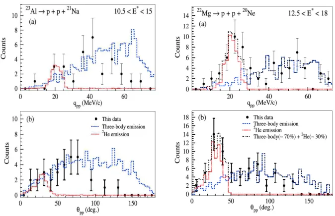
β-delayed emission of two protons (β2p decay) was first discovered in the TZ = −2 nucleus 22_{Al by Cable et al. in 1984 [Cab84]. The βp decay of this proton-rich Al isotope was already}

established as were several proton-unbound levels in the β-decay daughter 22_{Mg. The results}

by Cable et al. included a measurement of the energies of the individual proton groups. These energies were identified as one-proton transitions to and from unbound levels in the daughter

21_{Na, while the sum corresponded to the energy expected for a two-proton decay from the IAS}

to both the ground state and the first excited state in 20_{Ne. Figure 1.5 shows the energy-sum}

and the individual proton spectra. The order of the individual proton transitions was deduced from the Doppler-shift induced by the kinetic energy of the recoil ion after the first proton emission. This was the first identification of a β-delayed sequential two-proton emission from an IAS. As explained above, one of the main interest in the β2p is to be able to determine if the decay proceeds by a sequential emission of single protons or a direct and simultaneous emission of two protons. New experimental techniques have since been developed to identify the decay sequence that will be described in detail below.

Figure 1.5 – (a) The total charged-particle energy detected in ∆E-E telescopes were measured and matches the expected values for a decay from the IAS in 22Mg to the ground state and the first excited state in 20_{Ne. The individual proton energies (x}

i, g′i) and (gi, g′i)were mesured and allowed

to determine the order of the one-proton decay paths to the excited state (b) and the ground state (c).

In Figure 1.6, predictions for many different β-delayed decay modes which have been, or could be, observed are presented. Most of β-delayed one-proton emitters with A < 60 have been observed (filled symbols in Fig. 1.6) and their decay Q-values and partial half-lives have

been measured. Based on the estimated Q-value of these decays, the lightest β2p and β3p candidates are 22_{Si and}23_{Si, respectively.}

As shown in Fig. 1.6, the β-delayed three-proton emitters are extremely rare and are even more difficult to observe because of the competition with other decay channels that involve less protons. Even if this process is less interesting from a nuclear-structure point of view, this decay channel could help to identify and measure the excitation energy of the isobaric analogue state. For now, β3p has been observed in only three nuclei : 31_{Ar [Kol14],} 45_{Fe [Mie07] and} 43_{Cr [Pom11a, Aud12] with decay branching ratios ranging from 0.1 to a few %. Figure 1.7}

presents the particle trajectories observed in a time projection chamber for these three decay paths (βp, β2p and β3p) following the decays of 45_Fe.

From the systematics in Figure 1.6, the Q3p-value for 23Si suggests a possibly observable

β3p decay branch. However, when several β-delayed decays are in competition, the more exotic branch is also the less probable. In Chapter 4, an experimental search for the β3p decay from

23_{Si will be presented in detail.}

1.3

One-Proton and Two-Proton radioactivity

In addition to β-delayed proton and multi-proton decays, direct single-proton emission from the ground state of nuclei were predicted in the early 1960’s [Zel60]. These decays occur when the Sp value is negative, and are referred to as proton radioactivity provided that the half-life

is sufficiently long enough. First cases of proton radioactivity were observed from an isomeric state in53_{Co, and from the ground states of}147_{Tm [Sch82],} 109_{I and}113_{Cs [Fae84]. Today, there}

are now more than 25 proton emitters that have been discovered. Based on the similarities with the Barrier-Penetration model already used to describe α-particle emission from ground states, it was found that the partial half-life for proton radioactivity depends primarily on the decay Q-value (Qp) and the angular momentum carried by the emitted proton. This

momentum is directly related to the single-particle orbit of the emitted proton. In addition, a nuclear-structure component that describes the wave-function overlap between the parent and the daughter must be applied. Because of the Coulomb barrier, which is determined by the charge of the nucleus, it becomes evident that single-proton radioactivity is more common in medium mass and heavier nuclei.

1.3.1

Two-proton radioactivity

Very quickly after his prediction of β delayed charged particle decays, Goldanksy [Gol61] pro-posed the existence of an even more exotic type of decay called two-proton radioactivity. This decay mode was predicted to occur from the ground states of even-Z nuclei close to the drip

Figure 1.6 – Survey of β-delayed particle decays from proton-rich nuclei through their IAS. the y-axis is the proton energy assuming an equal sharing of the available energy. Known emitters are indicated with filled squares while the open squares are those nuclei that have a favourable decay Q-value, but which have not (yet) been observed. In green, the lightest precursors and subject of the present thesis work 23Si and 22Si are highlighted. The solid blue lines indicate the limit where the competition between γ-decay and particle emission is expected to be significant. (Figure taken from Ref. [Bla08]).

Figure 1.7 – First observation of β-delayed three proton emission (c) from the ground state of45_Fe.

This rare decay mode is in competition with β+, βp (a) and β2p (b) decay channels. The branching ratio for β3p decay was measured to be 3.30% from 125 total decays. (Figure taken from [Pf¨u12]).

line, for which the pairing energy creates a unique situation where the Sp separation energy

is positive while the S2p value is negative. Decay by the emission of two protons is therefore

possible while the emission of a single proton is energetically forbidden. This is shown schemat-ically in Fig. 1.8. In this case, two-proton radioactivity cannot be a sequential decay through the one-proton daughter unless (as in light nuclei) the ground state of (A-1, Z-1) daughter is a very broad resonance. Sequential decay of two protons in this case could then occur through its low-energy tail.

Figure 1.8 – Schematic view of the two-proton radioactivity: the single-proton channel is forbidden because of the negative Qp-value, while the direct two-proton decay channel is open with respect to

the binding energies.

For direct two-proton emission, the partial half-life is determined by the height of the Coulomb and centrifugal barriers, and is therefore expected to be more probable in

medium-mass nuclei. The two-proton decay rate can be calculated using the same tunnelling model as used for α decay. The product of the two barrier-permeability exponentials, which translates into the probability that the charged particle will tunnel through the barrier can be written as:

ω = exp + −2π(Z − 2)e2√_m p !(E_pp " 1 ((ε) + 1 ((1 − ε) #, , (1.59)

where Epp is the total decay energy, and ε and 1 − ε correspond to the fractions of this total

energy that is available to each of the protons. The charge of the parent nucleus Z and the mass of the proton mp are also required. This distribution reaches a maximum when there

is an equal sharing of the proton energy (ε = 0.5). From this observation, two scenario were proposed to describe the nature of two-proton emission:

• the two emitted protons are correlated because of the pairing and nuclear interaction and form a l = 0 proton resonance. This system is not bound because of the Coulomb force and decays by emitting the two individual protons simultaneously.

• the process is a three-body decay where only energy and angular momentum conservation have to be respected. In this case, the angular distribution between the two protons is isotropic and the energy sharing distribution uniform.

One has to keep in mind that in addition to this simple kinematic aspect, the theoretical models must also take into account the structure of the parent and daughter nuclei, which tends to suppress the decay and increase the half-life. To be competitive with β+ _{decay, the proton}

emission half-life has to be faster. Known 2p emitters have half-lives that range from tens to hundreds milliseconds.

1.3.2

Discovery of Two-Proton Radioactivity

Ground-state two-proton radioactivity was discovered in 2002 in experiments performed simul-taneously at GANIL [Gio07] and at GSI [Pf03] following decays of45_{Fe. The secondary beams}

of 45_{Fe were implanted into a position-sensitive Si-strip detector that were surrounded by}

scin-tillators for the detection of β-particles. The experimental measurements used spatial and time correlations between implantation events and decay events in the Si detector to study and dis-criminate between the different decay modes. In these experiments, the 2 low-energy protons emitted following the 2p decay are stopped in the vicinity of the implantation and the energy recorded by the Si detector is always equal to their sum. One therefore expects to observe a peak in the charged-particle spectrum with a characteristic energy. Contrary to all β-delayed charged particle decays, a β-particle is not emitted following a true 2p decay. The width of a 2p peak is expected to be narrower than a βp peak since the latter is degraded by the summing of

the proton with some fraction of the energy deposited in the Si by the outgoing β particle. The experiments clearly showed that the 2p candidate peak was narrower than the widths observed for the βp peaks. By taking an anti-coincidence with the β-particle detectors that surrounded the Si, they also showed that this peak is not accompanied by a β particle. The β-particle anti-coincident proton energy spectrum obtained in the GANIL experiment [Gio07] is shown in Figure 1.9. The energy and the partial half-life of this transition were in good agreement with the various theoretical predictions as shown in the same Figure 1.9. All of these evidences were convincing enough to claim the discovery of this rare decay mode in 45_{Fe nearly 50 years}

after it was predicted to exist. Today, there are now 4 known 2p emitters: 45_{Fe (discovered in}

2002) [Gio07], 48_{Ni (2005, confirmed in 2011) [Dos05, Pom11b],} 54_{Zn (2004) [Bla05] and} 67_Kr

(2016) [Goi16].

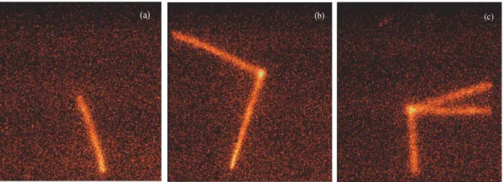
Following these discovery experiments that were not able to measure the individual proton energies and search for possible p-p angular correlations, experimental research in this field turned towards the development of a time projection chamber (TPC). After implanting the 2p precursor into a gas volume, the emitted protons will ionize the atoms or molecules of the gas all along their trajectories. The ionization electrons can be collected in an applied electric field onto a position-sensitive pad plane in order to provide a two-dimensional charge projection. The third dimension can be deduced using the time it takes the electrons to reach the pad plane. This method provides the means to create a full 3-dimensional image, on an event-by-event basis, which allows the decay channel to be clearly identified. In addition, the full kinematic reconstruction of each event can be used to deduce the individual energies of the emitted protons and measure the angle of emission between them.

The first direct observation of two-proton radioactivity from 45_{Fe in a TPC took place at}

GANIL in 2007 where a total of 10 implant-decay correlated events were identified [Gio07]. In a subsequent experiment at GANIL on 54_{Zn using the same device, 7 fully reconstructed,}

correlated implant-and-decay events were identified that allowed a measurement of the half-life and branching ratio that were in good agreement with a previous experiment using a Si detec-tor [Asc11]. Figure 1.10 presents a single event that was reconstructed in 3 dimensions. The TPC provided additional information on the energy and angular correlations between the emit-ted protons that was used to study the nature of the decay mode (sequential or simultaneous). Figure 1.11 (left) shows that the energy is equally shared between the two protons, which is in good agreement with the three-body model of Ref. [Gri00]. Figure 1.11 (right) compares the angular distribution between the two protons to the three-body model in order to estimate the nuclear shell orbital where the protons originated. The shell model was then added to include nuclear structure effects into the dynamics of the decay. By comparing the partial half-lives, they were able to conclude that nearly all of the 2p decay strength in 54_{Zn goes through the}

(0p)2 _{configuration.}

Figure 1.9 –The top figure presents the energy spectrum of the decay events recorded in a Si detector that were identified as two-proton decay from45Fe (taken from [Bla08]). The bottom figure compares the partial half-life deduced for the two-proton decay branch with different theoretical models (taken from Ref. [Gio07]).

but this decay mode can also occur from unbound excited states. These states can be populated from the β decay of a precursor (this is β2p decay that was described above) or from a nuclear reaction. Once the state is populated, and the 2p emission identified, the experimental goals are identical to the studies described above for ground-state 2p radioactivity. Measurements of the individual energies of the protons and the search for possible angular correlations between them provides unique insight as to the nature of this rare decay mode. The benefit to using a reaction to populate a 2p emitting state, as opposed to studying ground-state 2p decay, is the overall statistical yield. There are very few ground-state emitters known and their production cross sections are extremely small. One is often limited to overall yields of only ∼ 10 to 100 events

Figure 1.10 – The two-dimensionnal projection of the two proton trajectories (a) observed in the TPC after implantation of54Zn. The colors are here to indicate the energy loss detected in the strips. (b) The third dimension is obtained using the drift time of the electrons, allowing the measurement of the full kinematic. (Figure taken from [Asc11])

Figure 1.11 – The energy sharing bewteen the two charged particles is in good agreement with the three-body model of two-proton radioactivity. The angular distribution allows the identification of the two-proton initial orbitals. (Figures taken from [Asc11])

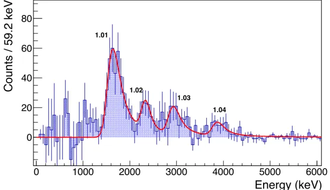
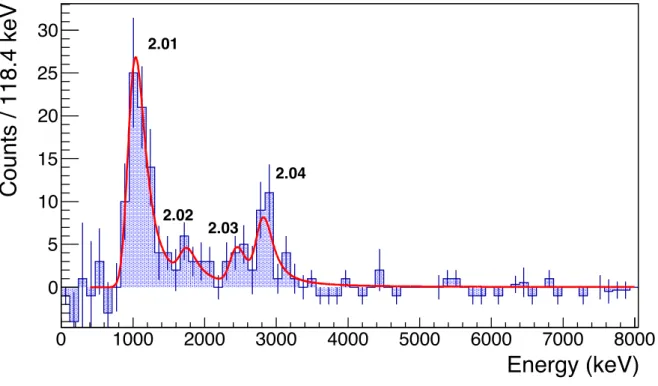
maximum after an experiment lasting several days. Depending on the β2p decay branching ratio or the reaction cross sections for populating these states, yields could be significantly higher. The other advantage, is that the energies of the protons emitted from excited states are much larger than the typical energies for ground-state decays (∼ 500 keV per proton) and thus their detection is conceptually simpler. An example of a reaction study to populate 2p emitting states in22_{Mg and}23_{Al was recently performed at RIKEN [Ma15]. Beams of}22_{Mg and}23_{Al were}

produced using the RIPS fragment separator and were sent to a12_{C reaction target. Following}

breakup reactions on the target, heavy fragments (20_{Ne and} 21_{Na, respectively) were identified}

using the Bρ − ∆E−TOF method, while the position and energy of the protons emitted from the excited states were measured using position-sensitive Si telescopes. Figure 1.12 shows the angular and energy correlations between the two protons that were obtained. The data were fitted using a Monte-Carlo simulation to identify whether the decays were two sequential single proton decays or the direct emission of two protons decay. The wide and isotropic energy and angular distributions that were measured for 23_{Al is in agreement with a sequential emission}

of two protons. However, the narrow angular distribution centered at 30◦

in22_{Mg is in better}

agreement with a simultaneous correlated process.

1.3.3

Summary and Motivation

Nuclei that are situated at, or close to, the proton drip line often exhibit several rare decay channels that are not open to nuclei closer to stability. These decay modes appear naturally from the combination of the increasing decay Q-values with the decreasing particle separation thresholds. Following the β decays of these near drip-line nuclei, branching ratios to particle unbound states give rise to β-delayed particle emission. Depending on the separation energies several different β-delayed decay channels may be open and can compete with each other. Delayed decays including βp, β2p, β3p, βα and βαp have all been observed experimentally. Delayed decay spectroscopy is an extremely useful experimental tool to study the structure of the unbound excited states in the daughter nuclei as they are populated with a reasonably high yield and these states can be inaccessible using other techniques such as transfer and scattering reactions or in-beam γ-ray spectroscopy. Studies of β2p decay can provide additional insight on the nature of the 2p-decay mechanism with higher statistical yield than ground-state 2p radioactivity that is produced with very limited intensities.

As described in this Chapter, the Coulomb force on the neutron-deficient side of the nuclear chart splits the degeneracy of an isospin multiplet of isobaric analogue states giving the highest energy to the lowest TZ member of the multiplet. It is then possible that the isobaric analogue

state decays to the ground state of the lowest TZ member is accessible through nuclear β+decay.

The use of β-delayed proton decay is also of crucial importance as the energy of this isobaric analogue state can be deduced via proton-decay spectroscopy. Once this key state is identified and its energy deduced, the isobaric mass multiplet equation (IMME) can be used to deduce

Figure 1.12 –Angular and energy correlations between the two protons emitted from the IAS in both

23_{Al and} 22_{Mg show two different decay mechanisms. An isotropic angular and energy distribution is}

observed for23Al which can be explained from a sequential decay of two protons. The peak observed in the case of22_{Mg suggests a strongly correlated simultaneous emission of 2 protons. (Figures taken}

from [Ma15]).

the masses for other unknown states of the multiplet. Measuring the energy of an IAS through its proton decay can thus be used to deduce the mass of the parent nucleus. Nuclear masses are essential and fundamental quantities in nuclear physics whose trends can be used to study the evolution of nuclear shell structure in unexplored regions of the nuclear chart, deduce the limits of nuclear binding and delineate the location of the drip lines, predict the onset of rapid shape changes and deformation effects and explore new and exotic decay modes.

As the single-particle separation energy gets even closer to zero, pairing effects can create situations where the nucleus is bound with respect to single proton emission but is unbound to the emission of two protons. Ground-state 2p radioactivity has now been experimentally observed in 4 cases (45_Fe,48_Ni, 54_{Zn and} 67_{Kr) and 2p emission from excited states populated}

either through the β2p decay channel or via nuclear reactions is a rapidly accelerating field. The big question surrounds the nature of the 2p decay mechanism and whether the protons are emitted sequentially or simultaneously. Recent technical developments in nuclear physics

include time projection chambers that have been extremely successful despite the difficulty associated with the overall statistical yield since the production cross sections for these exotic nuclei are very limited. The emission of 2 protons from excited states could yield higher statistics and the development of next-generation active targets (a TPC where the gas is also used as a reaction target) will certainly be an extremely efficient choice to continue with these types of experimental investigations.

In his original reviews of two-proton radioactivity [Gol61, Gol60], Goldansky proposed 22_Si

as the lightest possible candidate that could decay via this rare decay mode. Presently, very little is known about this nucleus. It is the lightest bound isotope with isospin projection TZ = −3 and is the most neutron-deficient Si isotope that is bound. It is known to β decay

with a half-life of approximately 30 ms [Bla97], which is short enough to allow the possibility of an appreciable 2p decay branch. The mass, however, has never been measured and so the S2p value can only be extracted from model extrapolations. Based on the current mass

evalu-ation AME2012 [Wan12], the two-proton separevalu-ation energy is S2p = −1200 (500) keV. In the

previous evaluation of AME2003 [Aud03], a value of S2p = −16 (202) keV was proposed. The

discrepancy between these two predictions and the large uncertainties do not permit any firm conclusions to be drawn. A precision mass measurement is clearly required to assess whether or not 22_{Si could decay by ground-state 2p radioactivity}

Because Si isotopes are refractory, the production of these nuclei using the isotope separation online technique (ISOL) is not possible. Laboratories such as ISOLDE at CERN and TRIUMF-ISAC in Vancouver that have powerful precision Penning traps to measure nuclear masses simply cannot produce the Si beams required. Production of Si beams can be achieved using in-flight fragmentation reactions at facilities like LISE at GANIL and the A1900 at NSCL but the half-life of 22_{Si is too short to allow these beams to be slowed down and injected into a}

trap. The only option to measure the mass of 22_{Si directly would be using the time-of-flight}

technique at a fragmentation facility but purifying the secondary cocktail beam would constitute a significant experimental challenge.

In this thesis, an indirect mass measurement using the β-delayed charged particle emission from the decay of 22_{Si will be presented. Secondary beams of the neutron-deficient nuclei} 20_Mg, 23_{Si and}22_{Si were produced at NSCL (MSU, USA) by fragmentation. After purification,}

the nuclei of interest were implanted into the Beta Counting System to detect the β-delayed protons and α particles. Identification of the daughter nuclei and the corresponding decay paths was performed using coincident γ rays that were detected in the 16 HPGe detectors of the Segmented Germanium Array (SeGA). In the next chapter (Chapter 2), the production of the secondary beam and the implantation-and-decay station will be presented along with the calibration techniques and the analysis program that will be used throughout this thesis. Chapter 3 presents the β-delayed decay spectroscopy of 20_{Mg that is a well-known decay and}