Computation of Higher-Order Hydrodynamic
Forces on Ships and Offshore Structures in Waves
by
Yonghwan Kim
BS in Naval Architecture and Marine Engineering, Seoul National University, 1987
MS in Naval Architecture and Marine Engineering, Seoul National University, 1989
Submitted to the Department of Ocean Engineering
in partial fulfillment of the requirements for the degree of
Doctor of Philosophy in Hydrodynamics
at the
MASSACHUSETTS INSTITUTE OF TECHNOLOGY
February 1999
©
Massachusetts Institute of Technology 1999. All rights reserved.
A uthor ... .. . .
-Depament of Ocean Engineering
OctoJyr, 1998
Certified by.
,Professor of
Paul D. Sclavounos
Naval Architecture
Thesis Supervisor
Accepted by...
-J--Kim
-andive
J. Kim Vandiver
Chairman, Departmental Committee on Graduate Students.... . .
MASSACHUSESMTE
OFT
Computation of Higher-Order Hydrodynamic Forces on
Ships and Offshore Structures in Waves
by
Yonghwan Kim
Submitted to the Department of Ocean Engineering on October, 1998, in partial fulfillment of the
requirements for the degree of Doctor of Philosophy in Hydrodynamics
Abstract
This thesis concentrates on the computation of hydrodynamic forces on ships and offshore structures. The specific topic of this thesis is the higher-order forces and moment. This thesis consists of two parts.
The aim of the first part is the development of a finite-depth unified theory for ship motions and its extension to the computation of the second-order mean-drift forces and moment. The mathematical background of the finite-depth unified theory is introduced, and an associated computer program is developed to verify this theory. The accuracy is checked from the comparison with the result of a three-dimensional panel code, and the nice agreement is shown. The theory is extended to the computa-tion of the second-order quantities. The mean forces and moment are computed using the far-field formulae, and the wave drift damping matrix is obtained by Aranha's
formula. Based on the present study, slender-body theory is shown to be a useful design tool for a floating ship, like an FPSO.
The second part develops a model and a corresponding computational program for the prediction of nonlinear wave effects. The primary interest is the second-order high-frequency effect which induces flexural body responses. The Rankine panel method using the bi-quadratic B-spline basis function is adopted as a method of solution. The theoretical aspects of the numerical scheme are described to verify the consistency and stability of the method, and a thorough parametric study is carried out. The computational result includes linear and nonlinear run-up and wave loads up to the second order. Based in this numerical method, the sum-frequency wave loads are obtained for a monochromatic wave and multi-frequency waves. Good agreement is shown with existing numerical and experimental data.
Thesis Supervisor: Paul D. Sclavounos Title: Professor of Naval Architecture
Acknowledgements
I would like to gratitude to everyone who supported my studies. First of all, my
deep appreciation must be directed to Prof. Sclavounos. I am always impressed by his sharpness and professional excellence. I have been blessed by the opportunity to study under his support. I am also greatly thankful to Prof. Yue and Prof. Makris, who served on my thesis committee and gave me good advice and fresh ideas.
This thesis is dedicated to my family. During almost two decades, my wife, Soo-jeong, has been always on my side with love. She is the only woman in my life, and her unconditional support led me up to this point. Soyeon and Ryan are my future. Their existence gave me strength when I was tired. I have an unpayable debt to my mother. Her sacrifice to my life cannot be more than anyone else, and it is always in
my mind.
I wish to thank all crews of our laboratory and the faculty of department. I
cannot forget the help and friendship of Dave, Yifeng, Alex ... . I hope they and their family have good luck and happiness in their lives. I also deeply appreciate Dr. Lee, C.H., who gave me advice in many respect. Also I will not forget the time spent with Korean 'gang'.
I acknowledge the financial support provided by Amoco, Aker, Conoco, DnV, Exxon, Norsk Hydro, Saga, Statoil, and ONR.
Contents
I
SLENDER-BODY THEORY
13
1 Introduction 14
2 Boundary Value Problem 18
3 A Finite-Depth Unified Theory 21
3.1 The Far-Field Solution ... 21
3.2 The Near-Field Solution ... . 23
3.3 Matching Conditions ... ... 25
3.4 The Kernel of the Integral Equation . . . . 27
3.5 Hydrodynamic Forces . . . . 30
3.6 The Equation of Motion . . . . 31
4 Second-Order Quantities 33 4.1 The Mean Drift Forces & Moment . . . . 33
4.2 Wave Drift Damping: Deep Water . . . . 35
5 Computational Results & Discussion 38 5.1 Solution Grid and Its Dependency . . . . 39
5.2 Hydrodynamic Forces . . . . 44
5.3 M otion RAOs . . . . 51
5.4 The Second-Order Quantities . . . . 57
II LINEAR & SECOND-ORDER FREE SURFACE FLOW
AROUND OFFSHORE STRUCTURES
6
1 Introduction
2 Boundary Value Problems
3 The Numerical Method
3.1 Rankine Panel Method . . . .
3.2 Stability Analysis . . . .
3.3 Wave Absorbing Zone . . . .
3.4 Conversion to Frequency Domain .
3.5 Spatial Filtering . . . .
4 Computational Results & Discussion 4.1 Solution Grid . . . . 4.2 Wave Absorbing Zone . . . .
4.3 Linear Radiation Problem . . . .
4.4 Linear & Second-Order Diffraction Problem : Monochromatic Wave . 4.5 Wave Loads at Irregular Waves . . . .
5 Conclusions & Contributions
A Fourier Transformation of A Finite-Depth Green Function
B Singularities on the Kernel
C The Extension of NIIRID to Finite Depth
D Body-Fitted Grid on Free Surface
E Artificial Wave Absorbing Zone
F Spatial Filters for Free-Surface Wave Problems
6
7 71 75 . . . . 75 . . . . 78 . . . . 85 . . . . 87 . . . . 88 91 . . . .- - - 9 1 .... . . . 9 5 . . . . 99 103 110 134 136 140 143 147 151 159List of Figures
2-1 Coordinate System . . . . 18
3-1 Comparison of the finite and infinite depth kernel, w = 1.0 . . . . 29 5-1 Solution grid for the Series 60 hull : (a) for unified theory, (b) for
W AM IT . . .. . .. . .. .. . . . .. . . . . . .. 41
5-2 Distribution of grid nodes on the parabolic Hull . . . . 41
5-3 Grid dependency on the heave added mass and damping coefficient : different number of sections, parabolic hull, h/L = 0.2 . . . . 42 5-4 Grid dependency on the heave added mass and damping coefficient :
different number of nodes, parabolic hull, h/L = 0.2 . . . . 42
5-5 Grid dependency on the second-order mean force : parabolic hull,
h/L = 0.2, = 180 . . . . 43 5-6 The heave added mass and damping coefficient: parabolic hull, infinite
depth . . . . 46
5-7 The heave added mass and damping coefficient: parabolic hull, h/L =
0 .2 . . . . 4 6
5-8 The pitch added mass and damping coefficient : parabolic hull, h/L = 0.2 47
5-9 The heave and pitch cross-coupled added mass and damping coefficient : parabolic hull, h/L = 0.2 . . . .. . 47
5-10 Effects of water depth on the heave added mass and damping coefficient : parabolic hull . . . . 48
5-11 Effects of water depth on the pitch added mass and damping coefficient : parabolic hull . . . . 48
5-12 The sway added mass and damping coefficient: parabolic hull, h/L =
0.125, strip theory . . . . 49
5-13 The yaw added mass and damping coefficient : parabolic hull, h/L = 0.125, strip theory . . . . 49 5-14 Wave excitation heave force (magnitude and phase) : Series 60, infinite
depth,
3
= 180 . . . ..50 5-15 Wave excitation pitch moment (magnitude and phase) : Series 60,infinite depth,
3
= 180 . . . .. 50 5-16 Heave RAO (magnitude and phase) : Series 60, infinite depth, 3 = 1800 535-17 Pitch RAO (magnitude and phase) : Series 60, infinite depth,
3
= 1800 535-18 Effects of water depth on the heave and Pitch RAOs (magnitude) :
parabolic hull,
#
= 1800 . . . .. 545-19 Heave and Pitch RAOs (magnitude) : parabolic hull, h/L = 0.2,
3
= 180' 545-20 Sway RAO at oblique sea (magnitude and phase) : Series 60, h/L =
0.125,
/
= 150 . . . ..555-21 Roll and yaw RAOs at oblique sea (magnitude and phase) : Series 60, h/L = 0.2,#= 1500 . . . . 55 5-22 Effects of the equivalent viscous damping on roll motion : Series 60,
infinite depth,
#
= 900, kA = 0.05 . . . . 565-23 Comparison of Kochin function with WAMIT : parabolic hull, h/L = 0.2, # = 1800 . . . . 60
5-24 Depth effects on the second-order mean force : parabolic hull,
#
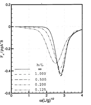
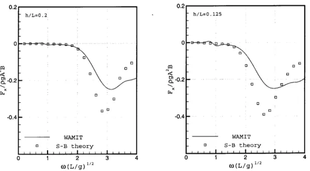
= 1804 60 5-25 Longitudinal mean drift force : parabolic hull, h/L = oc, 0.125,#
= 1800 615-26 Longitudinal mean drift force at oblique sea: Series 60, h/L = 0.2, 0.125,
/
=1500 ... ... 61 5-27 Lateral mean drift force at oblique sea: Series 60, h/L = 0.2, 0.125,
#
=5-28 Yaw mean drift moment at oblique sea: Series 60, h/L = 0.2, 0.125,
#
=1500 ... . - - . - - - - .. 62
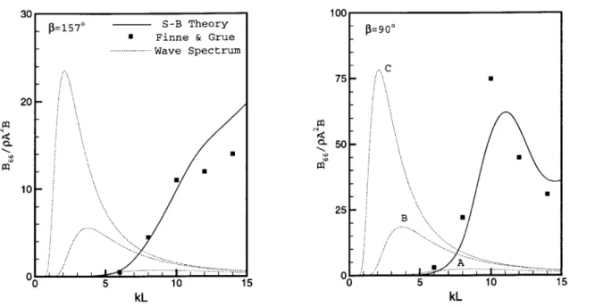
5-29 Yaw wave drift damping coefficients, B66, and ITTC wave spectrum
for L = 100m : ship1, infinite depth,
/3
= 1570(left) &/3
= 900(right),HS/L = 0.022(A), 0.05(B), 0.089(C), Tm(g/L)1/2 - 1.35(A), 2.51(B), 3.35(C) 63
5-30 Surge wave drift damping coefficients, B11 : ship1, infinite depth,
#
=1800 ... ... . 63
2-1 Coordinate System . . . . 72
3-1 Rectangular panels on free surface for stability analysis . . . . 79 3-2 Comparison of dispersion relation for the different order of basis
func-tion, a = 1.0,
#
= 1.0 . . . -. - . . . . 83 3-3 Contour plot of SO/4#2 and stability zone, a = 1.0, u = v . . . . 84 3-4 Application of the artificial wave absorbing beach . . . . 86 4-1 Solution grids : (a) a single bottom-mounted cylinder, (b) 4 truncatedcylinder . . . . 93 4-2 Solution grids for random waves near a bottom-mounted cylinder (half)
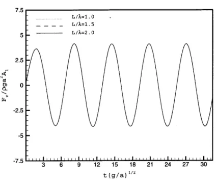
: (a) computational domain, (b) grids near the body . . . . 94 4-3 Linear horizontal force acting on a single truncated cylinder: w(a/g)1/2
1.0, L/A = 1.0, different damping strength . . . . 97
4-4 Linear horizontal force acting on a single truncated cylinder: w (a/g)1/2
1.0, po/w = 2.0, different zone size . . . . 97 4-5 Instantaneous second-order wave profiles for different damping strength
: w(a/g)1/2 = 1.0, L/A = 1.0, t(g/a)1/2 = 25.133 . . . . 98
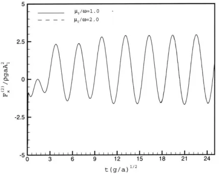
4-6 Second-order horizontal force acting on a single truncated cylinder :
4-7 Wave profile near a 4-cylinder array under forced surge motion : a/d =
1.0 for each cylinder, (x/D, y/D) = (1.5, 1.5), (1.5, -1.5), (-1.5, -1.5), (-1.5, 1.5),
w (D
/g)
= 2.0 -/2 . . . . 1004-8 Surge added mass and damping coefficient of a 4-cylinder array : the same array with Figure 4-7 . . . . 101
4-9 Heave added mass and damping coefficient of a 4-cylinder array : the same array with Figure 4-7 . . . . 101
4-10 Time-history of vertical force on a single cylinder in force heave motion with multi frequencies : a/d = 1.0, to/a = 0.05 . . . . 102
4-11 Added mass and damping coefficient for surge and heave motion : the same cylinder with Figure 4-10 . . . . 102 4-12 Wave profile near a bottom-mounted cylinder : diffraction problem,
a/d = 0.25, k1a = 2.0, A1/a = 0.2 . . . . 105 4-13 Contour profile of the diffraction potential near a bottom-mounted
cylinder : the same case with 4-13 . . . . 106 4-14 Time-history of horizontal force on a bottom-mounted cylinder:
diffrac-tion problem, the same cylinder with Figure 4-12 . . . . 107 4-15 Linear wave excitation force and moment on a bottom-mounted
cylin-der : the same cylincylin-der with Figure 4-12 . . . . 107 4-16 Module of surge QTF on a bottom-mounted cylinder : the same
cylin-der with Figure 4-12 . . . . 108 4-17 Wave run-up on (experiment) /near(computation) a bottom-mounted
cylinder : d/a = 2.768, k1a = 0.271, (a) A1/a = 0.244, (b)Aa/a = 0.397 108 4-18 Time-history of the vertical forces on a single truncated cylinder :
d/a = 2.075, k1a = 0.6, A1/a = 0.2 . . . . 109 4-19 Module of heave QTF on a single truncated cylinder: the same cylinder
4-20 Time-history of the second-order surge force on the cylinder at
bichro-matic waves : a bottom-mounted cylinder, h/a = 4, k1a = 1.0, k2a =
1.2, Ai,2/a = 0.1,
#1,2
= 180 . . . .. . . 1114-21 Time-history of the second-order surge force on the cylinder at
bichro-matic waves : a bottom-mounted cylinder, h/a = 4, k1a = 1.0, k2a =
1.6, Ai,2/a = 0.1, 11,2 = 1800 . . . ..111 4-22 Surge QTF obtained from the force signal of bichromatic waves : the
same cylinder with Figure 4-20, k1a = 1.0, 1.2(fixed), A1,2/a = 0.1,
#1,2
=1800 ... ... .. -. - .. 112
4-23 Time-history of the wave elevation, the linear and second-order surge force on the cylinder at multi waves: k1a = 1.0, 1.2, 1.4, 1.6, Ai,2,3,4/a =
0.1, 01,2,3,4 = 1800, no phase difference . . . . 114
4-24 Comparison of the diagonal sum-frequency surge QTF between
monochro-matic wave and multi waves : the same cylinder with Figure 4-23 . . 115
4-25 Four by four surge QTF matrix obtained from a single time history at multi waves : the same cylinder with Figure 4-23, different computa-tional domain, (a) sum-frequency (b) difference-frequency . . . . 116 4-26 Four by four surge QTF matrix obtained from a single time history at
multi waves : the same cylinder with Figure 4-23, different numbers of panels, (a) sum-frequency (b) difference-frequency . . . . 118 4-27 Four by four surge QTF matrix obtained from a single time history
at multi waves : the same cylinder with Figure 4-23, different time segments, (a) sum-frequency (b) difference-frequency . . . . 119
4-28 Four by four sum-frequency surge QTF matrix obtained from a single time history at multi waves : the same cylinder with Figure 4-23, different sampling time for the Fourier transform, above;TFT= Tmax,
4-29 Four by four difference-frequency surge QTF matrix obtained from a single time history at multi waves : the same cylinder with Figure 4-23, different sampling time for the Fourier transform, above;TFT = Tmax,
below;TFT= 2, 3, 4 XTmax . . . .. . . . 122
4-30 Four by four sum-frequency surge QTF matrix obtained from a sin-gle time history at multi waves : the same cylinder with Figure
4-23, different size of the artificial damping zone, (a) sum-frequency (b)
difference-frequency . . . . 123 4-31 Discretization of ITTC spectrum at sea state 5 in the North Atlantic
Sea : H, = 3.25m, Tm = 9.7sec, 20 components . . . . 125
4-32 Discretization of ITTC spectrum at sea state 6 in the North Atlantic
Sea : H, = 5.0m, Tm = 12.4sec, 20 components . . . . 125
4-33 The instantaneous linear and second-order wave profiles near a trun-cated cylinder : ITTC spectrum at sea state 5, d/a = 4.0 . . . . 126 4-34 Time signals of the linear wave elevation, linear and second-order forces
ITTC spectrum in Figure 4-31, from top ; wave elevation, the linear
surge and heave forces, the second-order surge and heave forces . . . 128
4-35 Time signals of the linear wave elevation, linear and second-order forces
: ITTC spectrum in Figure 4-32, from top ; wave elevation, the linear
surge and heave forces, the second-order surge and heave forces . . . 131
A-1 Line source along x axis at z = z . . . .. 137
C-1 Local coordinate system for a two-dimensional segment . . . . 144 D-1 Coordinate transformation for grid generation . . . . 149 D-2 The effect of forcing terms, (a) P(() < 0, (b) P( ) = 0, (c) P(s) > 0 150
E-1 A pulsating pressure patch problem . . . . 153 E-2 Evolution of free surface near a pulsating pressure patch : p,/w, = 27r,
E-3 Evolution of free surface near a pulsating pressure patch : quadratic
variation without P2 term (a) p10/wp = 27r, L/D = 1, (b) po/w, =
47r, L/D = 1, (c) p,/wp = 27r, L/D = 2, (d) pt/w, = 47r, L/D = 2 . . . 155
E-4 Evolution of free surface near a pulsating pressure patch : quadratic
variation, (a) p,/w, = 27r, L/D = 1, (b) p/w, = 47r, L/D = 1, (c)
pO/wp = 27r, L/D = 2, (d) po/Wp = 47r, L/D = 2 . . . . 157
E-5 Evolution of free surface near a pulsating pressure patch quadratic
variation with p2 term (a) puo/wp= 1, L/D = 0.5, (b) po/wp = 2, L/D =
PART I
Chapter 1
Introduction
During the last decade, most studies in marine hydrodynamics are based on nu-merical methods and the complete three-dimensional problems have been of interest. From today's point of view, slender-body theory may be too simplified or too mathe-matical to be used as a design tool. However, it cannot be overlooked that strip theory has been the most popular tool for the analysis of seakeeping performance over past two decades. The reason of this popularity is partly its reasonable accuracy. In spite of the fact that strip theory is a low-order theory, its accuracy is quite reasonable for the linear seakeeping analysis. Furthermore unified theory provides better accuracy comparable with three-dimensional method. More significant merit is its computing effort. A unified theory code supplies almost instant answer using very little memory. An another important but hidden reason is the simplicity of input data, in particular the treatment of the hull form. Slender-body theory requires the offset data on ship sections, so called, stations.
Recently second-order quantities have become important in the design of FPSO (floating production, storage, offloading ship) or shuttle tanker. One of the important issues in the design of these vessels is the slow drift motion, which is related to the design of a dynamic positioning system and/or mooring lines. Strip theory has been used to compute the added resistance which is a second-order quantity, but it doesn't provide accurate results for such quantities. Since the second-order quantities are very
sensitive to the accuracy of the linear solution, a method more accurate than strip theory is required even for the linear problem. In this sense, the three-dimensional panel code, like WAMIT or SWAN, is desirable for the computation of second-order quantities.
Unified theory bridges the gap between strip theory and a three-dimensional panel method. Unified theory has an advantage that sectional offset data are sufficient for the representation of the hull geometry. Furthermore the accuracy of unified theory is comparable with that of the dimensional method since it introduces a three-dimensional correction to strip theory. In addition the computation code requires much less CPU time than any three-dimensional panel code. Therefore unified theory may be an effective design tool which has all the advantages of strip theory and of a three-dimensional panel code.
The most pioneering work for ship motion using slender-body theory was done by Korvin-Kroukovsky and Jacobs [40]. Their method is based on the assumption of a long slender body and short waves, not taking into account the interaction between sections. Correcting Timman-Newman relation in their method, many refinements were introduced. The most popular strip theory may be the method used by Faltinsen, Tuck and Salvesen in 1970. A further development from strip theory was done by Newman [54] and Sclavounos [64] who gave an excellent exposition of the state of the art in this field. They presented a theoretical foundation perturbing from the strip theory approach, to extend the region of whole frequencies.
There are not many studies of the finite-depth seakeeping problem. Even though the shallow-depth effect on two-dimensional sections has been studied many times, few applications of the finite-depth strip theory exist. Kim [26] has shown the result of the finite-depth strip theory, and Tuck [75] introduced a theory which assumes that the depth is shallow and the wavelength is comparable with the ship length. Borresen
[6] has tried to extend unified theory to finite depth when the ship has forward speed.
He derived the far- and near-field solutions of the velocity potential, and an integral equation was proposed. However, he didn't show any meaningful results since the
kernel of his integral equation involves double-integral terms which are difficult to compute.
The present study is on the line of Borresen's work, in particular for a zero-speed case. When there is no forward zero-speed, the kernel of the integral equation can be simplified using a contour integral, and it can be written as a series form that makes the integral equation easy to solve. Unified theory is based on the matched asymptotic expansion method, and an integral equation is derived from matching the inner expansion of the far-field solution with the outer expansion of the near-field solution. Solving the integral equation, both the far- and near-field solutions can be completed. The present work introduces the far- and near-field behavior of the velocity potential around a slender ship in finite depth, and a new kernel is derived for the motion of the body with no forward speed.
Based on the present theory, a computer code has been developed for the heave and pitch motion of a slender ship. Since the solution of strip theory is necessary for unified theory, a strip theory code must be developed first. In the present study, NIIRID [68], a computer code developed for two-dimensional sections, was used for the strip theory code, and it was extended to the finite-depth problem. The series form is used for the two-dimensional finite-depth Green function. The unified theory code for the heave and pitch motions is extended from this strip theory code. Using the strip theory solution, the three-dimensional corrections are computed by solving the integral equations of unified theory. Numerical computations were carried out for a few typical slender ships. The hydrodynamic coefficients and motion RAOs are compared with WAMIT for validation.
The present study is extended to the computation of the second-order quantities. Since the accuracy of unified theory is comparable with that of three-dimensional panel method, the computation of the second-order mean forces and moment was carried out using the linear solution in unified theory. The accuracy of these quantities depends on the accuracy of Kochin function, i.e. the velocity potential and the motion RAOs. For the deep water problem, Kim & Sclavounos [33] applied the deep-water
unified theory (heave, pitch) and strip theory(sway, roll, yaw) to the computation of second-order quantities, and they showed a favorable agreement with WAMIT. The present study introduces the results for finite depth.
This study includes the wave drift damping for infinite depth. Aranha [2] sug-gested a formula for the wave drift damping coefficients in surge and sway. More recently he extended his formula to the yaw-motion component [3]. Although there is some doubt about its accuracy, particularly in the radiation problem, his formula has an advantage that it requires just the drift forces at zero speed. Computations were carried out for a mathematical hull, Ship1, which Finne and Grue [19] considered. The damping coefficients with Aranha's formula are compared with the result of the three-dimensional panel method obtained by Finne and Grue.
This part consists of five chapters including this introduction. In chapter 2 the boundary value problem is formulated with the fundamental assumptions. The theo-retical approach of the boundary value problem is described in chapter 3. In the far field, the velocity potential is written as the line distribution of a three-dimensional wave sources, while the near-field solution can be obtained by solving the two-dimensional boundary value problem formulated using the slender-body assumption. From matching two solutions, a new integral equation is derived. In chapter 4, the formulae for the second-order quantities are summarized. Using the linear solutions, the mean-drift forces and moment can be obtained using far-field formulae. The wave drift damping coefficients are also computed using the mean forces and moment at zero speed, and Aranha's formula is applied. The computational results based on the present theory are introduced in chapter 5. The hydrodynamic forces, motion RAOs and second-order quantities are computed for a few typical slender ships and the results are compared with WAMIT and other existing data.
Chapter 2
Boundary Value Problem
Consider a Cartesian coordinate system fixed in space with the free surface taken at z = 0. As shown in Figure 2-1, the center-plane of the ship is at y = 0 and
the positive x axis points towards the bow. Assume that the ship undergoes small harmonic oscillatory motions in a monochromatic linear wave with frequency w.
Figure 2-1: Coordinate System
the linear velocity potential, <b, is defined by <D(x, y, z, t) = R{#(x, y, z)e iW} (2.1) where 6 #(x, y, z) = RJ{# + #7 + E j#(x, y, Z)}. (2.2) j=1
The subscript
j
means the direction of motion, and (j is the complex motion am-plitude.j
= 1, 2, 3 andj
= 4, 5, 6 correspond to the translational and rotational motions.#7
denotes the diffraction potential and#,
is the incident wave potential given byigA cosh{k(z + h)} _ik(xcos#+ysin3). (2.3)
W cosh kh
A is the wave amplitude and
#
is the angle of the incident wave, with 3 = 1800 for head waves. k is the wave number.The linearized boundary value problem for
#j(x,
y, z) can be written as follows:- Fluid domain, V2
4j
= 0 (2.4) - Free surface, SF(Z 0),a#-
w
2 o - # = 0 (2.5) Oz g - Body surface, SB, fi j=1jinj... 6 (2.6) ion .jI
j =7- Bottom surface, Sh(z = -h),
a = 0
(2.7)
Oz
n = (ni, n2, n3) is the unit normal vector pointing inside the body surface with
n5= -xn + zni. This boundary value problem requires an additional radiation
condition to become well posed.
Chapter 3
A Finite-Depth Unified Theory
Unified theory is based on the matched asymptotic expansion method. Two dis-tinct solutions at the far and near field around a ship are described in the following sections. Their inner and outer expansions are major interests in order to match two solutions in the overlapping zone. The two leading terms are considered in the inner and outer expansions. The first term is a strip theory contribution, and the other term is a three-dimensional correction. The matching conditions produce an integral equation, which is a key of unified theory. In order to develop the present theory, the ship is assumed slender so that the longitudinal flow gradient near the ship hull can be assumed to be much smaller than the transverse flow gradients.
3.1
The Far-Field Solution
The velocity potential doesn't feel the detailed body shape in the far field, located at a radial distance comparable to or greater than the ship length. If a body is slender, the velocity potential can be expressed as a line distribution of three-dimensional finite-depth wave sources,
where q3(() is the strength of the Green function, G(x, y, z). Using the convolution
theorem,
#j
(x, y, z), can be rewritten in the Fourier domain as1 oc
# (x, y, z) = du eiuxq*(u)G*(u; y, z). (3.2)
27r -oo
The superscript * denotes the Fourier transformation.
G*(u; y, z) can be obtained by solving the boundary value problem for a line
distribution of wave Green functions, and the details are described in Appendix A.
G*(u; y, z) is written as follows :
1 00 G*(u; y, z) = o drJ dve" x 1 cosh{ u2 + v2(z+ h)} (3.3) cosh{ u2 + v2h} [ u2 + v2 tanh{ u2 + v2h} - v] where v = w2/g.
Equation (3.3) recovers the result of Ogilvie and Tuck [58] when h -+ oc,
1 ivy eMo
G*(u; y, z) - dvevY . (3.4)
27r J-oo V/U2 + v2 - *
Let's define a Fourier-transformed function, f*(u; y, z), such that
f*(u; y, z) = G*(u; y, z) - G*(0; y, z) (3.5)
Notice that G*(0; y, z) = G2D(y, z) where G2D(y, z) is the two-dimensional Green
function which satisfies the linearized free-surface boundary condition and the radia-tion condiradia-tion. Then the velocity potential can be rewritten as
#5j(x,
y, z) = G2D (y, Z)qj (X) +fQj - X'yZ)<. (3.6)The adoption of f(x, y, z) leads the decomposition of the far-field solution with two terms, two-dimensional and three-dimensional contributions. As mentioned later,
the near-field solution is supposed to be written as the same form.
Now consider the inner expansion of the far-field solution. The inner expansion can be obtained using the Taylor series expansion of the integral term in equation (3.6) for small y and z. The Taylor series expansion is applicable when a function is not singular at its expansion point. In this case, the expansion is applied to the integral. The integral of
f
( - x, y, z) doesn't have a singularity at ( - x, y, z) = (0, 0, 0), andthe details are explained in Appendix B. Then, the inner expansion is written as
<j(x, y, z) = qj(x)G2D(y, Z) + )f -j( X)0,0)<
+y g j (q)f(( - x, y, z)<jy=z=0
+Z'91 qj( )f (-x, y, z)dly=z=o + O(y2, z2) (3.7)
For the heave and pitch motion, the second integral term vanishes because of sym-metry. The third integral term remains as long as z is not zero.
3.2
The Near-Field Solution
At transverse distances of the order of the ship beam, the details of the ship geometry should be considered. In particular the relative orders of the flow gradients are dictated by the relative orders of the body surface gradients. If the body is slender for the y and z coordinates to be of O(e), the gradients in the longitudinal and transverse directions can be written as
-
0(1)
<< a, 7- =O(-).
(3.8)OX Oy 19z E
Then the boundary value problem is reduced to the two-dimensional problem at a certain section of the body.
Notice that the body boundary condition is pure imaginary. If there is a term which is pure real and satisfied with other conditions, it will be a homogeneous
solution. Then the general solution of the near field consists of a particular solution
#p
and a homogeneous solution#H,
#j(X, y, Z) = #j,P(x, y, z) + C (x) j,H (x, y, z) (3.9)
C(x) is an arbitrary function of x which will be determined from the matching with the inner expansion of the far-field solution. The particular solution is the strip theory solution, say @kj(xI y, z) which satisfies the pure imaginary body boundary condition. The homogeneous solution can be regarded as a free wave potential which is a pure
real potential, and Oj (x, y, z) + '/ (x, y, z) can be a homogeneous solution where Oj is the complex conjugate of $j. Thus we can rewrite as
#j(X, Y, Z) = {1 + C(x)}@(x, y, z) + Cj(x) (x, y, z) (3.10)
The outer expansion of this solution is of interest in order to match with the inner expansion of the far-field solution. At a large distance from the body, the particular solution has a point-source behavior. Then it can be written as
e0i
(x, y, Z) = o-j (x)G2D (Y, Z) (3.'1where o-(x) is the strength of the two-dimensional wave source, G2D, placed at the center of the section. Therefore the outer expansion of the near-field solution is written as
#j(x,y,z) = [o(x) + Cj(x){uo-(x) +j(x)}]G 2D(y,z)
- Cj (x)&(x)(G 2D(y, z) - 02D y, z)) (3.12)
with
. cosh{mo(z + h)} moh
cosh(moh) vh + (moh )2 COS(my)
+0( 1) (3.13)
y
and m = k, such that
v = mo tanh(moh) (3.14)
G2D - G2D contains the three-dimensional effects in the near-field solution. The
physical description of this term is a free wave contribution. When y becomes large, the local waves decay exponentially. In consequence the free wave contribution is dominant in G2D - G2D. Newman [54] showed the deep water case,
G2D(y, z) - 2D(y, Z) - 2i(1 + vz) cos(vy) (3.15)
when h -+ oc. This limit case is proven using
cosh{m0(z + h)} emoZ = 1 + moz + (mOz)2 +
... (3.16) cosh(moh) 1 ) 1 (3.17) vh +( cosh(m,, h) vh and v = m.
3.3
Matching Conditions
At a transverse distance greater than the body beam but less than the body length, the inner expansion of the far-field solution should be the same with the outer expan-sion of the inner-field solution.
Both equations (3.7) and (3.12) are decomposed with two terms, and the com-parison of each term leads two matching conditions. However, unfortunately, both equations include the z-coordinate. In order to circumvent the difficulty of treating
the z-coordinate terms, consider the matching conditions at z = 0. That is to say,
matching can be carried out on z = 0 and extended to z < 0 by analytic continuation. If the far- and near-field solutions should be the same, the coefficients of the
two-dimensional Green function should be the same,
qj(x) = oj (x) + Cj (x){o 3(x) + &j (x)}. (3.18)
The same applies to the three-dimensional correction terms,
F(qj) Jgj()f ( - x 1 0)d
= -2iCj(x)&(x) . (3.19)
vh + ( m ,h (2
The unknown parameter in the far-field solution is qj (x), while C (x) is unknown in the near field. Therefore the above two equations will supply the solutions of the two unknown parameters. The elimination of C (x) from the above equations leads to the integral equation for qj(x),
vh±+
(
m~h )2 ()}q)qj(x) + cosh(m)2{1 + }F(qj) = ou (x). (3.20)
2imoh & x)
The solution of the integral equation determines the far-field solution and also the complete near-field solution in the form
uj(x) -- o(x)
<pg (x, y, Z) = @yj (X, y, z) + aj _W {@,jW v (x, y, Z) + VNy (x, y, Z)} (3.21)
Equation (3.20) has to approach the deep water case when h -+ oc,
qj (x) - (- + 1)L(qj) = og (x) (3.22)
-where
L(q) q(x) (y + i7) +
IL
{
sgn(x - ) ln(2vlx - || d- - K[v(x - ()] q()
}
(3.23)4
and
K(x) = Y(|xj) + 2iJO(|x|) + Ho(|xj) (3.24)
Here, JO(x), Y(x) are Bessel functions of zero-th order and Ho(x) is Struve function of zero-th order. Besides, -y is the Euler constant.
F(qj) must approach L(qj) as h -+ oo. Since equation (3.13) approaches equation
(3.15), the limiting case can be proved by observing the kernel.
3.4
The Kernel of the Integral Equation
The computation of the kernel is the key in unified theory since the success of solving equation (3.20) depends on the computation of kernel. Borresen obtained the kernel in the Fourier domain in which the double numerical integration has to be carried out. In consequence, the triple numerical integration should be treated to solve this integral equation.
If the ship has no forward speed, a more simple form of the kernel can be derived.
Consider the Fourier-transformed kernel,
[00 f*(u;yz) = dv eVY x 27r -oo cosh{ u2 +v2(z + h)} cosh{ u2 +v 2h}[ u2 +v 2 tanh{ u2 +v 2h} - v] cosh{lvj(z + h)} (3.25) cosh(|vlh)[|v| tanh(|v~h) - v]
there are two poles on the !R(v) axis which contribute to the free wave. The poles on the Im(v) axis contribute to the local waves near a source singularity. When
y = Z = 0, f*(u;0,0) = m 1 mh -v2h+v 0 m2 _ 20 -Zmh vh m - 1) (3.26) nh +v2h - v m2 + 'Ub2 n=1 nl n where mntan(mnh) = -v (3.27)
which is the dispersion relation of the local waves. Using
J0
du eZiUX m -FiY, 0(MX) + wrJ 0(mx) (3.28)-oo m2 _ U2
du e- i m = 2KO(mx), (3.29)
-oo
Vm
2+
u2the kernel in the physical domain is written as
1 20
f
(X, 0, )= --f
*(u; 0, 0) e'"'du 27 -oo 1 m 2 2 {-iY(mox) + Jo(mox) - -6(x)} 2m h-v 2h+v mo - " n {-Ko(mnx) (x)} (3.30) n=m h+ v2h - v ,r mnwhere Ko(x) is the modified Bessel function of zero-th order.
Now, the kernel is written in a series form. In fact, this result is consistent with the series forms of the two- and three-dimensional Green functions derived by John
[25] and rewritten by Wehausen and Laitone [79].
re-quired. When y and z approach zero, the two-dimensional Green function has a logarithmic singularity and the three-dimensional Green function has the logarithmic and 1/r singularities. However, these singularities can be integrated. Furthermore the 1/r singularity is canceled out with the two-dimensional logarithmic singularity when it is integrated. The details are described in Appendix B.
Figure 3-1 shows the Fourier-transformed kernel,
f*
(u; 0, 0), for finite and infinitedepth. When h -+ oc, the kernel has to recover the infinite depth case. f*(u; 0,0) of the infinite-depth kernel takes the form :
2v 1
lim
f*(u;
0, 0) =ln(
-)
+ Iri-h-+oo u_
- i7r + cosh-1(!)
-7r + cos-1()
if v > |lu
ifv <jul
J
The finite-depth kernel approaches the infinite depth limit as h becomes large.
4.5
3.5
2.5L*0
U
Figure 3-1: Comparison of the finite and infinite depth kernel, w = 1.0
3.5
Hydrodynamic Forces
The added mass aij and damping coefficient bij can be obtained from the inner solution by integrating the linearized pressure over the body surface.
w2aij - iwbij = -iwp ni~ds (3.32)
where p is the water density.
Since the near-field solution can be decomposed with two separate terms, it follows that
-iwp ni5jds = Hi + H2 (3.33)
where
H1 = -i p nJibds (3.34)
H2 = -iwp f niC (x)(0 + 4')ds (3.35)
H1 is the contribution from strip theory, and H2 is the three-dimensional correction due to unified theory. Hence strip theory holds only H1. In the deep water problem,
when v -s oo, Cj(x) -+ 0 so that strip theory is recovered. The same is valid for the
finite depth case.
The other quantities of interest for the evaluation of ship motions are the wave excitation force and moment. Since the radiation potential is known, the Haskind re-lation is applicable. Combining the body boundary condition, the near-field Haskind relation is written as
Based on the Green's theorem, Sclavounos [67] derived the far-field Haskind relation,
Xi ipgA qj (x) eivxcos dx (3.37)
According to the study of Kim & Sclavounos [33], the far-field formula provides a more accurate result in slender-body theory.
3.6
The Equation of Motion
Assuming that linear surge mode of motion couples weakly with heave and pitch for slender ships, the classical equations of motion follow in the form
- Coupled Heave-Pitch Equations of Motion
-w 2
(M + a3 3) + iwb3 3 + C3 3 ]3 +
S-w 2(M35 + a3 5) + iwb35 + C35 ]Es = X3 (3.38)
-w 2
(M53 + as3) + iwb5 3 + C5 3 ]3 +
[ -w2(I5 + ass) + iwb5s + C
5 5 ]s - X5 (3.39)
- Coupled Sway-Roll-Yaw Equations of Motion
-w 2(M + a
2 2) + iw b22 + C22 ] 2 + S-w 2(M 24 + a24) + iwb2 4 +C 2 4 ](4 +
-w 2(M + a4 2) + iwb 42 + C4 2 ]2 + -w 2 (144 + a44) + iwb44 + C44 ] 4 + -w 2 (M 46 + a46) + iwb46 + C46 X4 (3.41) -w 2(M + a62) + iwb62 + C62 ]2 + -w 2(M64 + a64) + iwb64 + C64
](4
+ [ -w2(I + a6 6) + iwb66 + C66 ](6 =(3.42)
M, Iij are the mass and moment of inertia of ship. Cij means the restoring term.
CD,eq is an equivalent coefficient of roll viscous damping.
The added masses and damping coefficients for sway, yaw and roll are obtained by strip theory suggested by Salvesen, Tuck and Faltinsen [62]. Also all other quantities which unified theory is not available are computed using their method.
The roll motion is greatly affected by fluid viscosity which has a nonlinear be-havior. The state of the art of roll damping mechanisms is described in the report of Himeno [22]. In the present study, the concept of equivalent drag coefficient is applied. The equivalent linear damping can be obtained by preserving the energy loss by viscous effects, and it can be written as
CD,eq = CD4W (3.43)
37
where CD is the quadratic viscous damping coefficient. Note that CD,eq is a function
of motion frequency and amplitude. Hence, at a given frequency, an iterative scheme is applied to get the amplitude of roll motion.
Chapter 4
Second-Order Quantities
4.1
The Mean Drift Forces & Moment
The slow drift forces and responses are important factors for the design of an off-shore structure and a floating ship, like an FPSO. The accurate prediction of drift force is essential to design a mooring and/or dynamic positioning system. In the sim-ulation of the slow drift motion, the mean force and moment are the most important quantities. They may be obtained using only the linear solution.
For deep water, the surge and sway mean forces can be obtained by the far-field equations suggested by Maruo [46].
2_ f27r1
P = |20 H (0)12 cos OdO + - pwA cos ,3 R{ H(r + ,3)} (4.1)
87r o0 2
fv2 21r 1 1
810
=H(6) 2 sin OdO + pwA sin 3 R{H(-r + )} (4.2)
where H(O) is the infinite-depth Kochin function defined as
H() - # v(z-icosO-iYsin 0)dS (4.3)
be rewritten in the following forms :
P= p 2 27r 2
v8 f |IrH (0)| 2(COs n + cs O)d6
Fy = V2 7 H(() |2 (sin 0 + sin O)d6
(4.4)
(4.5)
The yaw moment, MA can be obtained using the equation derived by Newman
[52].
2 =-Im 21r(O)
OH()d6
-IlpwA
Im{ O9 (7r+3)}
where R(0) means the complex conjugate of H(9).
In finite depth, the far-field momentum formula is written as (C.C.Mei [47])
, - = - pgAgA- C[ 2 Cg z = mo C42 C9 X 1 z [4Z2 1Z2
J0
27r z2 27r|Hh(0) 2 cos Od9 + Z cos 3 Im{Hh(w +
m)}
] (4.7) Hh(0)12 sin 9d9 + Z sin 3 Im{ Hh(7r +m)}
] (4.8)1Mf27rfh0 Ba (0) d~ ImH0(9 d96 1 OHh(7 + 09 (4.9) C9 C 2 2 Z - - V cosh2(moh) v2h -mh - v {1+ 2moh 2 sinh(2moh) and Hh(9) is the finite-depth Kochin function, defined as
( o - < 19) e-imo(xcos9ysino)cosh{mo(z+h)}ds. Oan n cosh(moh) (4.6) where (4.10) (4.11) Hh (0)
=I
(4.12)Particularly when there is no external work done to the ship,
x
= pgA' C9 x [ --Z2f Hh ()1 2(cos O + cos#)dO ] (4.13)mA C x 4 1 0
pgA=
- 9 - x ±[Z2 f2| Hh(O)12(sin96 + sin #d6]. (4.14)
mo C 47r o0
The diffraction velocity potential is also required to compute the Kochin function.
In the present study, the diffraction potential is replaced with the velocity potential of
an equivalent two-dimensional wave-maker problem. At first, the diffraction problem based on strip theory is solved. Then the integral equation, equation (3.20), is solved using the strip theory solution. Since equation (3.20) applies to the radiation problem, this method can be considered as the wave-maker problem of a snake-like vessel. That
is to say, the ship is set to an equivalent wave maker with a wavelength of 27r/v cos
#.
So the diffraction potential is corrected approximately based on this idea.
4.2
Wave Drift Damping: Deep Water
The wave drift damping coefficients can be computed using Aranha's formula which is based entirely upon the knowledge of the drift forces at zero speed. Aranha's formula is valid only in deep water. In the present work, a wave drift damping matrix is obtained using the mean drift forces and moment by unified theory for deep water. The wave drift damping coefficient, Bj, is defined in the drift matrix equation for a ship with small forward speed.
I
x,u (w,
3)Fx (w,30)]
y,U (w, y(w,/3)
Biu(w,
3)
- B2 1(w, #) B61(w, #) B12(w,/#) B1 6(w,3) B22(w,#) B26(w, #) B62(LO ) B66(W, )where Pu, Pyu, Mp are the drift forces and moment when the ship has a steady speed, Ux, Uy, and Qz. Aranha's formula
[2]
provides thatw OF =-cos3o: -2sin 3
g
a(.4
OFx0#
=-[sin~o I+ 2cos# 3 g au#O
= OF-g[c05/3w- -2sin/3 w OFY S [sin w O g -[cos Ow g Bo -[sin/# g 8M WOW y a/3 + 2 cos 0/ 3+
aoM
-
2 sin3 0 /or
-4cos#I
-4 sin PFx] -4cos# PY] 4 sin#
Py] + 4 cos3 RZ] + 4 sin AzMThe first differential terms consider the change of wave frequency caused by the forward speed and the second terms consider the change of wave angle. There are two differential terms in equation (4.16), and these are obtained using a central difference formula.
The third column of the drift damping matrix, Bi6, can be obtained by the recent Aranha's formula [3] which is based on the slender-body approximation.
B16(w,
/3)
B26(w,/) B66(w,/)
B2 (w,3 -1 2 ~ B62(w,#) ~ B2 2(w,/3) (4.17) UI UV QzI
(4.15) Biu(w,#) B12(w, ) B2 1(w,#) B2 2(w,3)
B6 1(w,3)
B62(w,3)
(4.16)where
fL 2{1 _ (a( 2
' = (4.18)
fL{1 __ 2
b(x) is the water-line profile of the ship.
Even though Aranha's formula is not conclusively proven to be exact, especially for the radiation problem, it has been found to provide quite accurate predictions of the drift damping coefficients for offshore structures.
Chapter 5
Computational Results &
Discussion
In order to develop a computer code of unified theory, a strip theory code is essential. For the present computation, the strip theory code developed at MIT for deep water was extended for finite depth. The infinite-depth code is based on NIIRID for the evaluation of the sectional added mass and damping coefficient. NIIRID solves the complete boundary value problem for an arbitrary two-dimensional section. In the computation of the finite-depth problem, the subroutine of NIIRID, which computes the Green function, is extended to finite depth. The finite-depth Green function was evaluated using a series form. The details about the extension are described in Appendix C.
Numerical computations were carried out for a few slender ships. A mathemat-ical hull and a Series 60 hull are considered for the linear and mean drift quan-tities. The mathematical hull is of parabolic shape, like the Wigley hull, with beam(B)/length(L)=0.15 and draft(T)/length(L)=0.1. The Series 60 hull has the block coefficient (CB) of 0.7, and a parent model is considered. For the wave drift damping coefficients, computations were performed for the mathematical ship used
by Finne and Grue [19]. This hull, called Ship1, is expressed by the 4-th order
5.1
Solution Grid and Its Dependency
Since unified theory is a slender-body theory, sectional offsets are only necessary for the description of the hull geometry. Figure 5-1 shows the stations for slender-body theory and the three-dimensional mesh for WAMIT on the Series 60 hull. Figure 5-2 shows the distribution of grid nodes on the parabolic hull.
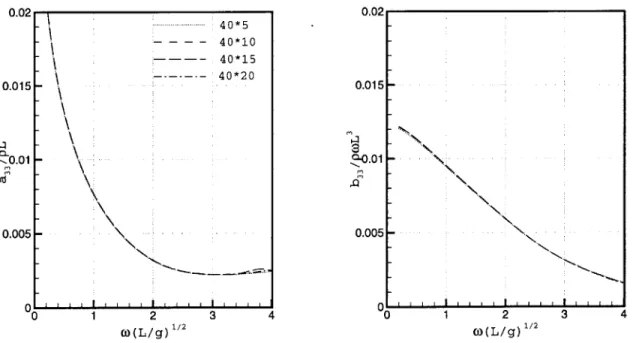
Figure 5-3 shows the dependency of section number on the heave added mass and damping coefficient for the parabolic hull. In this case, the number of nodes on each section is fixed. Figure 5-4 shows the effect of node number with the fixed number of sections. Both results show the insensitivity of solution grid for linear quantities. Table 1 compares the values for one specific case, w L/g = 2.0. It is surprising that the result with 5 stations and 3 nodes on each section is not much different with the that of 40 stations and 20 nodes. Even for a mathematical hull form, this result is quite encouraging.
Table 5.1: The heave added mass (half domain) ; parabolic hull, h/
(a33) and damping coefficient(b33)
L = 0.2, w(L/g)1/2
- 2.0
for different grids
station node a33 b33____ 3 3.1767739E-03 5.7931738E-03 5 5 3.1702337E-03 5.7432665E-03 10 3.1910257E-03 5.7664076E-03 5 3.1650849E-03 5.8484091E-03 10 10 3.1855819E-03 5.8818124E-03 15 3.1951349E-03 5.8921375E-03 5 3.1638728E-03 5.8937315E-03 20 10 3.1846275E-03 5.9162732E-03 15 3.1943801E-03 5.9264624E-03 5 3.1635107E-03 5.9003350E-03 30 10 3.1850706E-03 5.9226453E-03 15 3.1948064E-03 5.9333052E-03 10 3.1848375E-03 5.9254845E-03 40 15 3.1948953E-03 5.9358547E-03 20 3.1997717E-03 5.9412871E-03
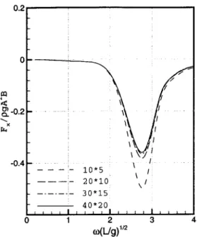
The grid dependency on the second-order quantities has to be observed since these has a shorter length scale than the linear quantities. Figure 5-5 shows the convergence of the longitudinal mean force on the parabolic hull. The results shows more sensitivity on the number of station. However, the grid dependency on the second-order quantities are not serious so that usually more than 20 stations provides a nice convergence.
(a)
(b)
Figure 5-1: Solution grid for the Series 60 hull: (a) for unified theory, (b) for WAMIT
Parabolic Hull
5 stations & 3 nodes in half body
20 stations & 10 nodes in half body
0.015 0. '0.01 0.005 0 1 2 (j)(L/g) 1/2 3 0.02, 0.015 3.01 0.005 4 0 1 2 W(L/g) 1/2
Figure 5-3: Grid dependency on the heave added mass and damping different number of sections, parabolic hull, h/L = 0.2
0.015 0.01 0.005 O 1 2 0o(L/g) 1/2 3 4 0.02 0.015 0.01 0.005 "0 1 2 0)(L/g) 1/2 3 coefficient : 3
Figure 5-4: Grid dependency on the heave added mass and damping coefficient different number of nodes, parabolic hull, h/L = 0.2
10*10 20*10 30*10 - --N N - N - N - N N K K K I ~ I, 40*5 - - - -40*10 40*15 -- -- 4 0*20 0K 20 -N N - N - N N - N - N N. - N. N N K K K K .3 I I I E.. I I I I I I I I I I I I - " 13111 t
0.2 0-2-0.2 --1 -0.4 105 20*10 -..- .- 30*15 40*20 I I I I 0 1 2 3 4 co(Ug)"2
Figure 5-5: Grid dependency on the second-order mean force: parabolic hull, h/L =
5.2
Hydrodynamic Forces
The accuracy of the hydrodynamic forces depends on that of velocity potential. Since the computation of the hydrodynamic forces requires the surface integration of the velocity potential on ship sections, the accurate velocity potential guarantees the accurate hydrodynamic forces. The accuracy of the velocity potential is also related with the second-order quantities, and it will be mentioned later.
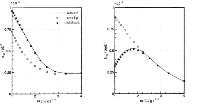
Figure 5-6 plots a33 and b33 for deep water, and these are compared with the
results of strip theory and WAMIT. It is obvious that strip theory is not suitable at low frequencies.
Figure 5-7 and 5-8 compare the heave and pitch added mass and damping coeffi-cients. It is obvious that the present unified theory provides an accuracy as good as the deep water case. In particular, at low frequency, the strip theory solution shows a large discrepancy with those of WAMIT and unified theory.
Strip theory is valid in the high frequency range. When the wave length is large compared with the ship length, the three-dimensional effect becomes more significant so that strip theory is not good as much as in the high frequency range. These results show clearly the weak point of strip theory. The same trend can be observed in Figure
5-9 for the heave-pitch cross coupling terms.
Depth effects on the heave added mass and damping coefficient are shown in Figure
5-10 and 5-11. At low frequencies, the hydrodynamic coefficients are very sensitive
to depth.
The hydrodynamic coefficients of other motions are shown in Figure 5-12 and 5-13. These results are by strip theory, and there is some discrepancies in both motions.
Figure 5-14 and 5-15 shows the wave excitation forces and moment in head waves. These results are for deep water, and the far-field Haskind formula is applied in this computation. The same accuracy is found in the finite depth problem. As expected, unified theory shows a good agreement with WAMIT. For the motions where unified
*102 0 0.5 -- 0 0.5 ---o 0 00 0.25 - 0.25 -01 2 3 4 2 3 4 O(L/g) 1/2 O(L/g)12
Figure 5-6: The heave added mass and damping coefficient : parabolic hull, infinite depth - 0 --U 0 1 2 3 4 o(L /g)1/
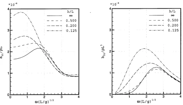
Figure 5-7: The heave added mass and damping coefficient : parabolic hull, h/L = 0.2 0.02 0.015 0.01 0.005 0.04 0.03 CO.02 0.01 0(L/g) 1/2 " *10- 2
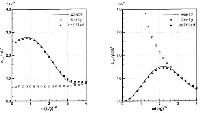
4.0. WAMIT o Strip . Unified 3.0- 2.0- 1.0-n 0 00 0 0 0 0 0 0 0 I nn[ 1 2 3 o(L/g)1"2 4 S 0. 2 (L/g)'1
Figure 5-8: The pitch added mass and damping coefficient : parabolic hull, h/L = 0.2
*10~' 4*10~4 2 0o(L/g) 1/2 S 0. 0o (L/g) 1/2
Figure 5-9: The heave and pitch cross-coupled added mass and damping coefficient: parabolic hull, h/L = 0.2
0~