HAL Id: hal-01231887
https://hal.archives-ouvertes.fr/hal-01231887
Submitted on 21 Nov 2015
HAL is a multi-disciplinary open access
archive for the deposit and dissemination of
sci-entific research documents, whether they are
pub-lished or not. The documents may come from
teaching and research institutions in France or
abroad, or from public or private research centers.
L’archive ouverte pluridisciplinaire HAL, est
destinée au dépôt et à la diffusion de documents
scientifiques de niveau recherche, publiés ou non,
émanant des établissements d’enseignement et de
recherche français ou étrangers, des laboratoires
publics ou privés.
Audio synchronisation with a tunnel matrix for time
series and dynamic programming
Jan Gorisch, Laurent Prevot
To cite this version:
Jan Gorisch, Laurent Prevot. Audio synchronisation with a tunnel matrix for time series and
dy-namic programming. 40th IEEE International Conference on Acoustics, Speech and Signal Processing
(ICASSP), 2015, Brisbane, Australia. �hal-01231887�
AUDIO SYNCHRONISATION WITH A TUNNEL MATRIX FOR TIME SERIES AND
DYNAMIC PROGRAMMING
Jan Gorisch
?†Laurent Pr´evot
??
Aix Marseille Universit´e & CNRS, Laboratoire Parole et Langage, France
†
Nanyang Technological University, Division of Linguistics and Multilingual Studies, Singapore
ABSTRACT
Precise multimodal studies require precise synchronisation between audio and video signals. However, raw audio and audio from video recordings can be out of sync for several reasons. In order to re-synchronise them, a dynamic program-ming (DP) approach is presented here. Traditionally, DP is performed on the rectangular distance matrix comparing each value in signal A with each value in signal B. Previous work limited the search space using for example the Sakoe Chiba Band (Sakoe and Chiba, 1978). However, the overall space of the distance matrix remains identical. Here, a tunnel trix and its according DP-algorithm are presented. The ma-trix contains merely the computed distance of two signals to a pre-specified bandwidth and the computational cost is equally reduced. An example implementation demonstrates the func-tionality on artificial data and on data from real audio and video recordings.
Index Terms— Audio-video Synchronisation, Image-loss Compensation, Tunnel Matrix, Tunnel DP-algorithm, Storage Requirements
1. INTRODUCTION
The number of studies that analyse audio and video signals has increased with the attempt to account for the multimodal-ity of social interaction involving amongst others speech and gestures [1, 2] and investigations into the natural habitat of speech: face-to-face interaction. Although conversation an-alysts often have to restrain themselves to low quality audio and video recordings in order to preserve the naturaleness of talk-in-interaction [3], studies in interactional phonetics [4] that combine qualitative and quantitative methods by ap-plying computation techniques on automatically extracted features, e.g. Kurtic et al. [5] Gorisch et al. [6] and Bertrand et al. [7], require high quality audio recordings from close-speaking microphones. The audio has to be synchronised
Thanks to the ANR funding the project “Conversational Feedback” (grant number ANR-12-JCJC-JSH2-006-01). This research was supported in part by the Erasmus Mundus Action 2 program MULTI of the European Union, grant agreement number 2010-5094-7. Comments from St´ephane Rauzy were very much appreciated.
with the video recordings, if the multimodality of talk should be analysed for the same data. Usually, precautions are taken to ensure high standards for audio-video synchronisation, such as by Edlund et al. [8] who enhanced their recording setup and included a rotating turntable with an LP-disk that was scratched at a certain place and a visible marker. Au-dio and video signals were then synchronised in subsequent steps in order to render the data analysable. The analysis of desynchronised audio and video signals, however, is almost impossible. One source of error can be a clocking differ-ence of two recording devices that capture the same scene. Another source of error can be the hardware equipment it-self. For example, video recordings or capturing systems that imply MiniDV technology regularly introduce errors, i.e. a loss or surplus of image frames. Both problems were en-countered with recordings of a multimodal speech corpus [9]. Previously, such problems have been tackled by inserting or deleting frames at specific places by hand, as was performed for the CID corpus [10]. A more efficient and re-usable solu-tion that does not have to involve addisolu-tional equipment, such as turntables, was envisaged for the alignment of the signals, as e.g. of the audiovisual MapTask corpus [9].
2. APPROACH
The advantage of video recordings is that the camera usually includes an audio channel that captures the same scene as the separate audio recordings do. It means that two similar sig-nals of the same quality, i.e. acoustics, exist for the computa-tion of their alignment. Thus, the aim for synchronising audio and video is to insert or delete images from the video accord-ing to the alignment of the audio signals that stem from two different devices.
Dynamic Programming (DP) and Dynamic Time Warping (DTW) are methods that can be applied here, as they are used to align time series in an optimal way. They allow to deter-mine where one signal has to be stretched in time or shrunk in time in order to match the other signal [11]. These meth-ods had their revival in speech processing in recent years, e.g. with algorithms that search for re-occurring acoustic patterns for modelling infant speech acquisition [12] and algorithms that evaluate the similarity in prosodic patterns of
conversa-tional participants performing basic social actions [13]. De-velopments have been performed by Salvador and Chan [14] who increased the time efficiency of DTW algorithms. They solved a similar problem by matching two acoustic signals in order to synchronise them with a video signal. However, a problem of limited space and computational cost remains unsolved.
2.1. Space and computational cost problem of DP Many DP problems today take large time series as underlying data. For example, an attempt to align audio recordings of the length of half an hour (1,800s), even using a relatively sparse sampling rate of 25 samples/s (as standard video frames), re-sults in a distance- or similarity matrix of (25 × 1, 800)2, that
are 2,025,000,000 value pairs. Additional to the space re-quirements of this matrix comes the computational cost of dynamic programming to evaluate the best alignment path of the two underlying vectors. The Sakoe Chiba Band [15] or the Itakura Parallelogram [16] are techniques that can help to reduce that computation by limiting the search space to a band around the diagonal of that matrix from the start point to the end point of the underlying vectors.
One problem of current matrix processing is the limited storage space that is available on e.g. personal computers. Sometimes, it is physically not possible to create the distance matrix for two time series. Fortunately, this is even not nec-essary because the majority of values are not required in the case for the audio-out-of-sync problem. If the DP algorithm that is supposed to be applied to such data is not required to look at the edges of the distance matrix, that space is used without need. A sparse matrix, as introduced by Gilbert et al. (1992) [17], could be used in order to implement such a band. However, DP has not been demonstrated on sparse matrices, yet. In order to save space and computation power to solve the desynchronisation problem at hand, a new structure for the values of the distance matrix is suggested in section 3. 2.2. Conceptual and aesthetic problem
A more conceptual and probably aesthetic problem of a rect-angular distance matrix (1) is the distribution of the axes.
a1b1 a1b2 a1b3 a1b4 a1b5 a1b6 a1b7 a1b8 a1b9 a2b1 a2b2 a2b3 a2b4 a2b5 a2b6 a2b7 a2b8 a2b9 a3b1 a3b2 a3b3 a3b4 a3b5 a3b6 a3b7 a3b8 a3b9 a4b1 a4b2 a4b3 a4b4 a4b5 a4b6 a4b7 a4b8 a4b9 a5b1 a5b2 a5b3 a5b4 a5b5 a5b6 a5b7 a5b8 a5b9 a6b1 a6b2 a6b3 a6b4 a6b5 a6b6 a6b7 a6b8 a6b9 a7b1 a7b2 a7b3 a7b4 a7b5 a7b6 a7b7 a7b8 a7b9 (1) While one time series evolves along the x-axis and the other time series evolves along the y-axis, the overall time evolves along the diagonal. This is traditionally visualised with two vectors, e.g. ~a = a1a2. . . a7and ~b = b1b2. . . b9that combine
in a distance matrix as shown in (1) with time elapsing for ~a top–down, for ~b left–right and for overall time from top– left to bottom–right. From a conceptual point of view where time elapses from left to right, or from top to bottom, the traditional matrices, as they are produced by Matlab or R,R
are not optimal in this sense. Both, the reduction of the search space and the orientation of the time axis can be realised by introducing a tunnel matrix that represents the Sakoe Chiba Band (shaded area in (1)) rotated by 45 degrees to the left for horizontal or to the right for vertical propagation of time. This paper proposes an implementation of such a distance matrix in tunnel form at the initialisation stage, i.e. already before the calculation of the alignment path.
3. IMPLEMENTATION OF A TUNNEL MATRIX The aim is to rotate the Sakoe Chiba Band from a traditional distance matrix around the diagonal by −45 degrees in order to let time elapse from left to right. As can be seen in (1), the diagonal contains the isochronous pairs a1b1, a2b2, ... a7b7.
This should be the mid row of the new matrix. It can also be seen that the values of ~a are constant for each column of and increase from row to row. For ~b it is the inverse: the values are constant for each row and increase from column to column. In order to illustrate the new tunnel arrangement, two intermediate matrices are prepared. For all values of ~a and ~b that fall into the bandwidth of the Sakoe Chiba Band, a ‘tunnel A’ (2) and a ‘tunnel B’ (3) is created.
NA NA a1 a2 a3 a4 a5 a6 a7 NA a1 a2 a3 a4 a5 a6 a7 NA a1 a2 a3 a4 a5 a6 a7 NA NA a1 a2 a3 a4 a5 a6 a7 NA NA a1 a2 a3 a4 a5 a6 a7 NA NA (2) b1 b2 b3 b4 b5 b6 b7 b8 b9 NA NA b1 b2 b3 b4 b5 b6 b7 b8 b9 NA NA b1 b2 b3 b4 b5 b6 b7 b8 b9 NA NA NA b1 b2 b3 b4 b5 b6 b7 b8 b9 NA NA NA b1 b2 b3 b4 b5 b6 b7 b8 b9 (3)
For illustration purposes, a width of three values in each di-mension was chosen. Both intermediate matrices are then merged in order to create the final AB Tunnel Matrix by cross-multiplying ‘tunnel A’ and ‘tunnel B’, as shown in (4). Note that these values represent here similarity instead of distance.
NA NA a1b3 a2b4 a3b5 a4b6 a5b7 a6b8 a7b9 NA a1b2 a2b3 a3b4 a4b5 a5b6 a6b7 a7b8 NA a1b1 a2b2 a3b3 a4b4 a5b5 a6b6 a7b7 NA NA NA a2b1 a3b2 a4b3 a5b4 a6b5 a7b6 NA NA NA NA a3b1 a4b2 a5b3 a6b4 a7b5 NA NA (4)
4. THE TUNNEL DP-ALGORITHM
For the newly created similarity matrix, the traditional DP al-gorithms are inappropriate. The start point (a1b1) and the end
point (a7b9) are no more at the same location. And therefore,
the possible directions that an alignment path might take are also different. For a traditional similarity matrix, the most common step-pattern is from a1b1to a2b2without insertion
or deletion, to a1b2by insertion in ~a or to a2b1by insertion in
~b (or deletion from ~a).
This translates into the new tunnel matrix, however it has to be adapted depending where in the matrix the algorithm is currently working. The principle is the same: it is merely possible to continue in both vectors or to stay at the same value in one vector while proceeding in the other. In the mid row of the tunnel matrix, imagine to start at a1b1 in (5), the
steps indicated by arrows are possible. In the top half of the matrix (imagine the prior step went from a1b1to a1b2),
one arrow points into a different direction. That means the possible steps are different. In the bottom half of the matrix (imagine the prior step went from a1b1to a2b1), again, arrows
point in different directions.
NA NA a1b3 a2b4 a3b5 · · · NA a1b2 a2b3 a3b4 a4b5 · · · a1b1 a2b2 a3b3 a4b4 a5b5 · · · NA a2b1 a3b2 a4b3 a5b4 · · · NA NA a3b1 a4b2 a5b3 · · · (5) In order to find the path through the whole Similarity Matrix with the highest quality (inverse of cost), DP accumulates for each point of the matrix the maximum quality path up to that point in a Quality Matrix. Therefore, at each point of that ma-trix, the previously accumulated quality is added to the cur-rent similarity. The direction from where the lowest cost path came from is memorised in order to find the way back, once the whole matrix has been passed. The algorithm for filling the Quality Matrix according to the similarity matrix is again different from the traditional procedure. It is not possible to proceed row wise and column wise from one corner of the matrix (formerly the start point) to the opposite corner (for-merly the end point), even if the step-patterns are clear for each point. Because the DP algorithm always looks back-wards from the current point in order to evaluate the high-est quality path and accumulates in the current point the new quality-to-this-point, all possible points from where the path can come from need already be evaluated. If they are not, the new evaluation would be based on both, points that include the accumulated similarities (the quality) and points that have stored the mere individual similarity. This would bias the
de-cision in favour of the latter. A solution is suggested in the following section.
4.1. Quality Tunnel Matrix and Backtrack Matrix A Quality Matrix Q stores the accumulated similarities. A Backtrack Matrix φ stores at each point the direction from where the path with the highest quality came from. In a first step, Q is filled with the values of the similarity matrix SM and surrounded on top, bottom and left column, by a line of NAs (Not Applicable). This border is necessary in order to have initial values to be compared with. Once the DP algo-rithm has finished, the end point of that matrix contains the overall quality for the alignment of the two vectors ~a and ~b. The algorithm iterates over the columns via j and over the rows via i. Q(i, j) is the point in the Quality Matrix for which the accumulated quality is to be calculated, i.e. the maximum quality that accumulates until that point. As mentioned above, it is important that each time a potentially proceeding path is evaluated for the maximum quality, the values are either part of the border, or already filled. Therefore, a specific evalua-tion pattern is established.
An overall trend from left to right is used in order to reach from the start in the first column to the end in the last column. The rows are divided into three parts. The first part is the top half of the matrix, the second part is the bottom part of the matrix and the third part is the mid row. The rows of the top and bottom part are evaluated from the outside to the middle. For the top part (6), it means that i increases from 2 to the middle − 1 (row above the mid). For the bottom part (7), it means that i decreases from the end − 1 (previous last row) to the middle + 1 (row below the mid). At the last iteration per column, the value of the mid row is evaluated (8).
The following comparisons are performed for the three parts at each point Q(i, j). NAs (Not Appliccable) are in-serted in the diagrams in order to keep the indexing function for the backtrack path constant: The horizontal step is always 1, the vertical steps are always 3 (top) and 5 (down), and the diagonal steps are always 2 and 4. The lowest value is added to the current point Q(i, j). The direction from where this highest quality path came from is added to the Back-track Matrix at point φ(i, j). Arrows with solid lines indicate valid steps; arrows with dashed lines indicate invalid steps. The top half of the matrix (row 2 to mid − 1) evaluates Q(i, j) = max(Q(i, j − 1) + 2 × SM (i, j), NA, Q(i − 1, j) + SM (i, j), Q(i + 1, j − 1) + SM (i, j), NA).
NA Q(i − 1, j) + SM (i, j) Q(i, j − 1) + 2 × SM (i, j) Q(i, j) Q(i + 1, j − 1) + SM (i, j) NA 1 2 3 4 5 (6)
The bottom half of the matrix (row end − 1 to mid + 1): Q(i, j) = max(Q(i, j − 1) + 2 × SM (i, j), Q(i − 1, j − 1) + SM (i, j), NA, NA, Q(i + 1, j) + SM (i, j)).
Q(i − 1, j − 1) + SM (i, j) NA Q(i, j − 1) + 2 × SM (i, j) Q(i, j)
NA Q(i + 1, j) + SM (i, j) 1 2 3 4 5 (7) The mid row of the matrix is analysed last per column it-eration and evaluates: Q(i, j) = max(Q(i, j − 1) + 2 × SM (i, j), NA, Q(i − 1, j) + SM (i, j), NA, Q(i + 1, j) + SM (i, j)).
NA Q(i − 1, j) + SM (i, j) Q(i, j − 1) + 2 × SM (i, j) Q(i, j)
NA Q(i + 1, j) + SM (i, j) 1 2 3 4 5 (8) 5. EVALUATION
The new tunnel DP-algorithm applied to the tunnel matrix structure is evaluated on both artificial data and real data from recordings. The artificial data (invented for demonstration purposes) contains a matrix of values between 0.1 and 0.9 that are represented on a grey scale (left of Figure 1). The
Fig. 1. Evaluation of the new DP algorithm on artificial data. Similarity Tunnel Matrix left, Quality Tunnel Matrix right. DP-algorithm found an optimal alignment path (white line) by accumulating similarity scores in a quality matrix (right of Figure 1). The path through the regions of relatively high similarity demonstrates that the algorithm works well on arti-ficial data. Similar results are achieved on real data from the MapTask corpus [9] (using spectral information) from record-ings from devices with clock differences and random image loss (Figure 2). It can be seen that after approximately 4000 frames (25/s), one signal is approximately 27 frames behind, or the other ahead respectively. The Tunnel Matrix and the Tunnel DP-algorithm achieve alignment paths (as output) that
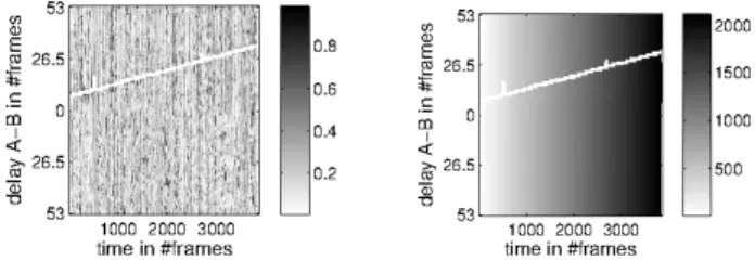
Fig. 2. Evaluation of the new DP algorithm on real data. Sim-ilarity Tunnel Matrix left, Quality Tunnel Matrix right.
follow high similarity regions as expected. The path can be used in order to align faulty video streams to intact audio be-cause the areas of image loss or surplus are well indicated. This method was successfully used to synchronise 90% of the recordings. The remaining 10% could not be recovered yet, as entire minutes of the video are lacking.
6. DISCUSSION
Matlab allows to indicate which parts of a matrix do not need to be stored in a “sparse” matrix [17], i.e. areas of numbers that are zero. However, DP on such sparse matrices has not been demonstrated yet. It means that the proposed architec-ture for optimised use of space is still lacking in programming languages such as Matlab. Even the function spdiags() does not achieve this. A functioning workaround is demon-strated here that applies a tunnel matrix with the according DP algorithm for synchronising audio signals. There are lim-itations, as for example gaps of the video spanning several minutes, that increase again the space requirements drasti-cally. But as long as the errors in the signal remain within reasonable limits (the range of several seconds), the algo-rithm can calculate an output (an alignment path) that can be used subsequently to align the video, e.g. by calling FFmpeg (http://ffmpeg.org) to copy or delete frames.
7. IMPLICATIONS AND APPLICATIONS Hardware failure of recording equipment is besides human failure a source for frustration and cost explosion for data repair. Previous work with the aim to prevent this has in-troduced even more hardware [8] that can also fail and that decreases the naturalness of social interaction additionally to the recording situation itself. Data that was recorded with less precautions should still be made available at a maximum pos-sible quality. One further step into this direction is achieved with the technique suggested in this paper. This DP-technique can also be applied in fundamental research that investigates the similarity of interacting participants on multiple parame-ters: acoustic-prosodic features investigating social alignment on a turn-by-turn basis [6] or on a larger time-scale as in en-trainment [18] or convergence [19], EEG and EMA signals or simple re-occurring patterns in the acoustics [20].
8. REFERENCES
[1] Tanya Stivers, “Stance, alignment, and affiliation dur-ing storytelldur-ing: When nodddur-ing is a token of affiliation,” Research on Language and Social Interaction, vol. 41, no. 1, pp. 31–57, 2011.
[2] Sigrid Norris, Analyzing Multimodal Interaction: A Methodological Framework, Routledge, New York, USA, 2004.
[3] Ian Hutchby and Robin Wooffitt, Conversation Analy-sis, Polity, Malden, MA, USA, 2008.
[4] John Local, “Phonetic detail and the organisation of talk-in-interaction,” in Proceedings of the Sixteenth International Congress of Phonetic Sciences (ICPhS), Saarbr¨ucken, Germany, 2007.
[5] Emina Kurtic, Guy J. Brown, and Bill Wells, “Re-sources for turn competition in overlapping talk,” Speech Communication, vol. 55, no. 5, pp. 721–743, 2013.
[6] Jan Gorisch, Bill Wells, and Guy J. Brown, “Pitch con-tour matching and interactional alignment across turns: an acoustic investigation,” Language and Speech, vol. 55, no. 1, pp. 57–76, 2012.
[7] Roxane Bertrand, Ga¨elle Ferr´e, Philippe Blache, Robert Espesser, and St´ephane Rauzy, “Backchannels re-visited from a multimodal perspective,” in Proceed-ings of the International Conference on Auditory-Visual Speech Processing (AVSP2007), Kasteel Groenendaal, Hilvarenbeek, The Netherlands, 2007.
[8] Jens Edlund, Jonas Beskow, Kjell Elenius, Kahl Hellmer, Sofia Str¨ombergsson, and David House, “Spontal: A Swedish spontaneous dialogue corpus,” in Proceedings of the Seventh International Conference on Language Resources and Evaluation (LREC’10), Malta, 2010.
[9] Jan Gorisch, Corine Ast´esano, Ellen Gurman Bard, Brigitte Bigi, and Laurent Pr´evot, “Aix Map Task corpus: the French multimodal corpus of task-oriented dialogue,” in Proceedings of the Ninth International Conference on Language Resources and Evaluation (LREC’14), Reykjavik, Iceland, 2014.
[10] Roxane Bertrand, Philippe Blache, Robert Espesser, Ga¨elle Ferr´e, Christine Meunier, B´eatrice Priego-Valverde, and St´ephane Rauzy, “Le CID – Corpus of Interactional Data – Annotation et exploitation multi-modale de parole conversationnelle,” Traitement Au-tomatique des Langues (TAL), vol. 49, no. 3, pp. 105– 134, 2008.
[11] Lawrence Rabiner and Biing-Hwang Juang, Fundamen-tals of Speech Recognition, Prentice-Hall, Inc., Engle-wood Cliffs, NJ, USA, 1993.
[12] Guillaume Aimetti, A Computational Model of Early Language Acquisition: A Data-driven Approach In-spired by the Empiricist View of Cognitive Development, Ph.D. thesis, The University of Sheffield, 2011.
[13] Jan Gorisch, Matching across Turns in Talk-in-Interaction: The Role of Prosody and Gesture, Ph.D. thesis, The University of Sheffield, 2012.
[14] Stan Salvador and Philip Chan, “FastDTW: Toward ac-curate dynamic time warping in linear time and space,” in The Third SIGKDD Workshop on Mining Temporal and Sequential Data (KDD/TDM 2004), Seattle, WA, USA, 2004, pp. 70–80.
[15] Hiroaki Sakoe and Seibi Chiba, “Dynamic program-ming algorithm optimization for spoken word recogni-tion,” IEEE Transactions on Acoustic, Speech and Sig-nal Processing, vol. 26, no. 1, pp. 43–49, 1978.
[16] Fumitada Itakura, “Minimum prediction residual prin-ciple applied to speech recognition,” IEEE Transactions on Acoustic, Speech and Signal Processing, vol. 23, no. 1, pp. 67–72, 1975.
[17] John R. Gilbert, Cleve Moler, and Robert Schreiber, “Sparse matrices in matlab: Design and implementa-tion,” SIAM Journal on Matrix Analysis and Applica-tions, vol. 13, pp. 333–356, 1992.
[18] Mathias Heldner, Jens Edlund, and Julia Hirschberg, “Pitch similarity in the vecinity of backchannels,” in Proceedings of Interspeech 2010, Makuhari, Japan, 2010.
[19] Spyros Kousidis, David Dorran, Yi Wang, Brian Vaughan, Charlie Cullen, Dermot Campbell, Ciaran McDonnell, and Eugene Coyle, “Towards measur-ing continuous acoustic feature convergence in uncon-strained spoken dialogues,” in Proceedings of Inter-speech 2008, Brisbane, Australia, 2008.
[20] Guillaume Aimetti, Roger K. Moore, and Louis ten-Bosch, “Discovering an optimal set of minimally con-trasting acoustic speech units: a point of focus for whole-word pattern matching,” in Proceedings of In-terspeech 2010, Makuhari, Japan, 2010.