Location extraction from tweets

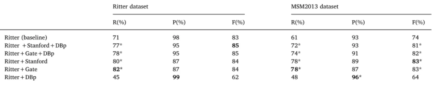
Our evaluation using the cor- pus shows that the conventional NE recognizer is insuffi- cient for understanding location phrases in chatting situa- tion, but the conventional method

This paper describes our approach on “Information Extrac- tion from Microblogs Posted during Disasters” as an attempt in the shared task of the Microblog Track at Forum for

Worth of hydraulic and water chemistry observation data in terms of the reliability of surface water-groundwater exchange flux predictions under varied flow conditions.7.

The main result of the paper is introduction of new exploiters- based knowledge extraction approach, which provides generation of a finite set of new classes of objects, based on

rules represent grammar pattern, implemented by finite state machines, typically used in both written and spoken language, thus several agents can be coordinated in a pipe and

Pérez-Pellitero, Javier; Universitat Rovira i Virgili, Departament d'Enginyeria Química Ungerer, Philippe; Institut Français du Pétrole Mackie, Allan; Universitat Rovira i

The extraction of a 3D topological map from an Oriented Boundary Graph can be needed to rene a 3D Split and Merge seg- mentation using topological information such as the

This paper proposes a P2P-based communication framework to realize geographical location oriented networks called G- LocON. An outline image of the proposed system is shown in Fig.

References

Agarwal, P., Vaithiyanathan, R., Sharma, S., & Shroff, G. (2012). Catching the long-tail: Extracting local news events from twitter. ICWSM.
Backstrom, L., Sun, E., & Marlow, C. (2010). Find me if you can: Improving geographical prediction with social and spatial proximity. Proceedings of the 19th international conference on world wide web. ACM61–70.
Bo, H., Cook, P., & Baldwin, T. (2012). Geolocation prediction in social media data byfinding location indicative words. Proceedings of COLING1045–1062.
Bontcheva, K., Derczynski, L., Funk, A., Greenwood, M. A., Maynard, D., & Aswani, N. (2013). TwitIE: An open-source information extraction pipeline for microblog text. RANLP83–90.
Cano Basave, A. E., Varga, A., Rowe, M., Stankovic, M., & Dadzie, A. S. (2013). Making sense of microposts (# msm2013) concept extraction challenge. Proceedings of the concept extraction challenge at the workshop on‘Making Sense of Microposts’ co-located with the 22nd international World Wide Web conference (WWW’13). Chandra, S., Khan, L., & Muhaya, F. B. (2011). Estimating twitter user location using social interactions-a content based approach. Privacy, security, risk and trust (PASSAT)
and 2011 IEEE third inernational conference on social computing (socialcom), 2011 IEEE Third International Conference on838–843. Etzioni, O., et al. (2005). Unsupervised named-entity extraction from the web: An experimental study. Artificial intelligence, 165(1), 91–134.
Finkel, J. R., Grenager, T., & Manning, C. (2005). Incorporating non-local information into information extraction systems by gibbs sampling. Proceedings of the 43rd annual meeting on association for computational linguistics. association for computational linguistics363–370.
Goeuriot, L., Mothe, J., Mulhem, P., Murtagh, F., & Sanjuan, E. (2016). Overview of the CLEF 2016 cultural micro-blog contextualization workshop. In experimental IR meets multilinguality, multimodality, and interaction. Proceedings of the seventh international conference of the CLEF association (CLEF 2016), Lecture Notes in Computer Science (LNCS) 9822. Springer, Heidelberg, Germany371–378.http://dx.doi.org/10.1007/978-3-319-44564-9-30.
Hall, M., Frank, E., Holmes, G., Pfahringer, B., Reutemann, P., & Witten, I. H. (2009). The WEKA data mining software: An update. ACM SIGKDD Explorations Newsletter, 10–18.
Hoang, T. B. N., & Mothe, J. (2017). Predicting information diffusion on Twitter-Analysis of predictive features. Journal of Computational Science.http://dx.doi.org/10. 1016/j.jocs.2017.10.010.
Huang, Y., Liu, Z., & Nguyen, P. (2015). Location-based event search in social texts. Computing, networking and communications (ICNC), 2015 international conference on668–672.
Ikawa, Y., Enoki, M., & Tatsubori, M. (2012). Location inference using microblog messages. Proceedings of the 21st international conference on world wide web. ACM687–690. Ji, Z., Sun, A., Cong, G., & Han, J. (2016). Joint recognition and linking offine-grained locations from tweets. Proceedings of the 25th international conference on world wide