Worth of hydraulic and water chemistry observation data in terms of the reliability of surface water-groundwater exchange flux predictions under varied flow conditions

HAL Id: insu-02935694

https://hal-insu.archives-ouvertes.fr/insu-02935694

HAL is a multi-disciplinary open access

archive for the deposit and dissemination of sci-entific research documents, whether they are pub-lished or not. The documents may come from teaching and research institutions in France or abroad, or from public or private research centers.

L’archive ouverte pluridisciplinaire HAL, est destinée au dépôt et à la diffusion de documents scientifiques de niveau recherche, publiés ou non, émanant des établissements d’enseignement et de recherche français ou étrangers, des laboratoires publics ou privés.

Worth of hydraulic and water chemistry observation

data in terms of the reliability of surface

water-groundwater exchange flux predictions under

varied flow conditions

Daniel Partington, Matthew Knowling, Craig Simmons, Peter Cook, Yueqing

Xie, Takuya Iwanaga, Camille Bouchez

To cite this version:

Daniel Partington, Matthew Knowling, Craig Simmons, Peter Cook, Yueqing Xie, et al.. Worth of hydraulic and water chemistry observation data in terms of the reliability of surface water-groundwater exchange flux predictions under varied flow conditions. Journal of Hydrology, Elsevier, 2020, 590, pp.125441. �10.1016/j.jhydrol.2020.125441�. �insu-02935694�

Journal Pre-proofs

Worth of hydraulic and water chemistry observation data in terms of the relia‐ bility of surface water-groundwater exchange flux predictions under varied flow conditions

Daniel Partington, Matthew J. Knowling, Craig T. Simmons, Peter G. Cook, Yueqing Xie, Takuya Iwanaga, Camille Bouchez

PII: S0022-1694(20)30901-X

DOI: https://doi.org/10.1016/j.jhydrol.2020.125441

Reference: HYDROL 125441

To appear in: Journal of Hydrology

Received Date: 7 November 2019 Revised Date: 19 March 2020 Accepted Date: 18 August 2020

Please cite this article as: Partington, D., Knowling, M.J., Simmons, C.T., Cook, P.G., Xie, Y., Iwanaga, T., Bouchez, C., Worth of hydraulic and water chemistry observation data in terms of the reliability of surface water-groundwater exchange flux predictions under varied flow conditions, Journal of Hydrology (2020), doi: https:// doi.org/10.1016/j.jhydrol.2020.125441

This is a PDF file of an article that has undergone enhancements after acceptance, such as the addition of a cover page and metadata, and formatting for readability, but it is not yet the definitive version of record. This version will undergo additional copyediting, typesetting and review before it is published in its final form, but we are providing this version to give early visibility of the article. Please note that, during the production process, errors may be discovered which could affect the content, and all legal disclaimers that apply to the journal pertain.

Worth of hydraulic and water chemistry observation data in terms

of the reliability of surface water-groundwater exchange flux

predictions under varied flow conditions

4

Daniel Partington1, Matthew J. Knowling2, Craig T. Simmons1, Peter G. Cook1, Yueqing

5

Xie1,3, Takuya Iwanaga4, Camille Bouchez5

6

7

1

National Centre for Groundwater Research and Training, & College of Science and 8

Engineering, Flinders University, Adelaide, Australia 9

2

GNS Science, Lower Hutt, New Zealand 10

3

School of Earth Sciences and Engineering, Nanjing University, Nanjing, China 11

4

Integrated Catchment Assessment and Management (iCAM) Centre, The Fenner School of 12

Environment and Society, The Australian National University, Canberra , Australia 13

5

Univ Rennes, CNRS, Géosciences Rennes, UMR 6118, 35000 Rennes, France 14

Corresponding author: Daniel Partington (daniel.partington@flinders.edu.au)

15

Abstract

17

This study assesses the worth of routinely collected hydraulic data (groundwater head, stream 18

stage and streamflow) and lesser collected water chemistry data (Radon-222, Carbon-14, 19

electrical conductivity (EC)) in the context of making regional-scale surface water-groundwater 20

(SW-GW) exchange flux predictions. Using integrated SW-GW flow and transport numerical 21

models, first-order, second-moment (FOSM) analyses were employed to assess the extent of the 22

uncertainty reduction or lack thereof in SW-GW exchange flux predictions following acquisition 23

of hydraulic and water chemistry observation data. With a case study of the Campaspe River in 24

the Murray-Darling Basin (Australia), we explored the apparent information content of these 25

data during low, regular and high streamflow conditions. Also, a range of spatial and temporal 26

prediction scales were considered: catchment-wide and reach-based spatial scales and annual and 27

monthly temporal scales. Generally, the data worth evaluations showed significant variability 28

across predictions that were dependent on the spatiotemporal scale of the SW-GW exchange, the 29

magnitude and direction of the SW-GW exchange flux and the prevailing streamflow conditions. 30

These dependencies serve to emphasise the importance of prediction specifity with respect to 31

SW-GW exchange. Among existing data, the most worth was found in Radon-222, groundwater 32

hydraulic head, EC,and streamflow data showing average reductions in uncertainty of 41%, 33

38%, 32%, and 23% respectively. Assessment of type and spatiotemporal locations of potential 34

data showed Radon-222 to be the next most important observation type across many predictions 35

in locations with data paucity of all data types. Hydraulic observation data types were found to 36

inform SW-GW exchange flux best under high- and regular- streamflow conditions when the 37

magnitude of exchange fluxes were largest, whereas the water chemistry data was of highest 38

value for low- and regular- streamflow conditions where groundwater is discharging to the 39

stream. 40

1 Introduction

41

Observation data underpins effective water resource management, and managers have 42

significant responsibility in decisions around data collection strategies. Conjunctive surface 43

water (SW) and groundwater (GW) resource management requires having a quantitative insight 44

into SW-GW exchange flux. Furthermore, the models that support such management are often 45

required to provide the SW-GW exchange across multiple spatiotemporal scales. 46

Numerous methods exist for SW-GW exchange flux measurement and estimation 47

(Fleckenstein et al. 2010; Kalbus et al. 2006). Means of estimating SW-GW exchange include 48

direct methods (e.g., seepage meters), aimed at measuring the actual SW-GW exchange flux in-49

stream at a point. Direct methods are limited to very small spatial scales less than a few square 50

metres and cannot be extrapolated to reach or regional scale SW-GW exchange (Cook 2015). 51

Furthermore, such methods are limited by difficulty in identifying net SW-GW exchange – as 52

opposed to hyporheic flow – and thus have limited utility at larger spatial scales (e.g. kilometre 53

scale and greater). 54

The estimation of SW-GW exchange along stream reaches, as opposed to at a point, 55

include methods based on stream water balance, hydraulic head gradient, river chemistry and 56

ground water chemistry (see review by Cook 2015). The stream’s water balance (through 57

differential gauging) can be used where the SW-GW exchange is a significant component of the 58

stream’s water balance, greater than any uncertainties associated with other components of the 59

balance. SW-GW exchange can be estimated by Darcian flux based on the average hydraulic 60

head gradient across the stream and the average hydraulic conductivity of the streambed/aquifer. 61

The exchange can also be estimated with stable and radioactive geochemical tracers (Cook 62

2013), requiring information on features such as the flow in the stream, stream geometry, and 63

hyporheic cycling. Electrical conductivity (EC) is one stable tracer that, given significant 64

differences between the GW and SW EC can be used with end-member mixing analysis to 65

estimate inflow of GW to a stream (Barthold et al. 2011). The presence of Radon-222 (222Rn) in 66

SW is indicative of GW discharge (Ellins et al. 1990), in the absence of significant hyporheic 67

flow. When the concentration of 222Rn in the GW is measured at multiple locations along a 68

stream along with adequate sampling in the SW, then areas of GW discharge at the time of 69

sampling can be pinpointed, and exchange fluxes estimated. As 222Rn is a gas with a half-life of 70

3.8 days, it will only remain in the stream for short periods of time. The conservative nature of 71

EC allows for differentiation of river water that briefly enters the streambed for a period before 72

returning to the stream, which with accumulation of 222Rn could be otherwise misinterpreted as 73

regional GW discharge. Thus it is possible that these two observation data types contain unique 74

information (i.e. uncorrelated) with respect to SW-GW exchange fluxes, which will be tested 75

herein. 76

The use of physically based numerical modelling of flow in SW-GW systems, which is 77

commonly applied to support managing water resources, allows for groundwater hydraulic head, 78

stream stage and streamflow data to be integrated (e.g., Schilling et al. 2018; Wöhling et al. 79

2018). Furthermore, coupling of transport to such a flow model affords further integration of 80

various stream chemistry and geochemical data, e.g. EC, 222Rn or 14C. Numerical models 81

simulating SW-GW exchange that support water resources management provide an important 82

basis for assessing the extent to which observations can build confidence in the prediction of 83

SW-GW exchange, i.e., data worth (Fienen et al. 2010). 84

The level of confidence in regional scale predictions of SW-GW exchange flux obtained 85

from various models is partly limited by the quality (measurement noise), quantity and types of 86

available data that inform such model predictions. Predictions of surface water-groundwater 87

exchange at a regional scale are critical to support conjunctive management of surface and 88

groundwater resources within strongly connected SW-GW systems, i.e. systems whereby change 89

to management of a river has a notable impact on the underlying aquifer and vice versa. 90

Determining the most informative observational data types and spatiotemporal quantities of such 91

data is an ever increasing need for water resource management practitioners (Kikuchi 2017). 92

The use of numerical models as a tool to formally assess the benefit of different data 93

types and optimal data acquisition/experimental design within a formal “data worth” assessment 94

framework is continually growing in popularity (Kikuchi 2017). The problem of “data worth”, in 95

the context of water resources modelling, can be defined in terms of the reduction or lack thereof 96

in the uncertainty of any key prediction of management interest that is afforded through the 97

acquisition of observation data. A popular method used is first-order, second-moment (FOSM) 98

analysis, which assumes the model behaves linearly with respect to its input parameters and 99

simulated outputs. This approach is commonly used because of its suitability to be applied in 100

combination with complex models (which are often used to support environmental management) 101

owing to its computational efficiency (e.g. Dausman et al. 2010; Fienen et al. 2010; Moore and 102

Doherty 2005). Brunner et al. (2012) used this approach to explore the worth of groundwater 103

hydraulic head, ET and soil moisture observations in informing regional scale groundwater 104

models. Wallis et al. (2014) demonstrated the utility of a FOSM-based data worth analysis of 105

bromide, temperature, methane and chloride in the context of aquifer injection trials following 106

coal seam gas-related water production. Schilling et al. (2014) investigated the utility of novel 107

tree ring data in reducing predictive uncertainty of SW-GW exchange. More recently, Zell et al. 108

(2018) used a similar approach to analyse groundwater hydraulic head, stream discharge, SF6,

CFCs and 3H in GW transport times. Finally, Knowling et al. (2019b), explored the worth of 110

tritium-derived mean-residence time data for forecasts of spring discharge. 111

In the current study, the worth of existing and potential different hydraulic and water 112

chemistry data are quantitatively investigated in the context of SW-GW exchange flux 113

predictions over monthly and annual timescales and over a range of length scales (whole of river 114

(141 km) vs reach (0.8 - 40.4 km)), for a field site in south-eastern Australia (Campaspe River 115

catchment). We specifically consider the worth of: groundwater hydraulic head, streamflow, 116

stream stage/depth, stream EC, stream 222Rn, and groundwater 14C for such predictions. To the 117

best of the authors’ knowledge, the benefit or otherwise of these tracer methods have not been 118

quantitatively evaluated compared to more traditional and routinely collected data types in the 119

context of SW-GW exchanges at the regional scale. This paper aims to answer: 120

Q1. To what degree, if at all, does the addition/omission of existing hydraulic observation

121

and/or chemical observation data reduce/increase the uncertainty of SW-GW exchange fluxes 122

and what is the spatiotemporal variability of such reductions/increases during low, regular 123

and high streamflow conditions? 124

Q2. Through consideration of potential future sampling locations and times, which hydraulic

125

and/or chemical data should be targeted in the future to yield the best reductions in 126

uncertainty of SW-GW exchange flux during low, regular and high streamflow conditions? 127

2 Case Study: Campaspe River

128

The Campaspe River, located in north-central Victoria, lies within the Murray-Darling 129

Basin, shown in Figure 1. The river runs for 220 km, beginning in the hilly terrain of the Great 130

Dividing Range and flowing down through undulating foothills to the wide flat riverine plain in 131

the north before it joins the Murray River; the river provides 0.9% of the inflow for the basin. 132

The Campaspe River overlies a series of alluvial aquifers, namely the Coonambidgal Formation, 133

Shepparton Formation, Calivil Formation and Renmark Group (the latter two also commonly 134

referred to collectively as the Deep Lead aquifer) which interact with the river along its length. 135

As shown in Figure 1, the hydrogeological units of the Lower Campaspe valley area are made up 136

of a Palaeozoic basement of fractured and faulted rocks, overlain by the Renmark Group which 137

contains a blanket of thinly bedded carbonaceous sand, silt, clay and peaty coal, then overlying 138

this is the Calivil Formation comprising coarse grained quartzose sand and gravel sheet with 139

minor kaolonite clay, and atop of the Calivil Formation the Shepparton Formation is made up of 140

fine-grained clastics and polymitic sand and gravel. Finally, incised into the Shepparton 141

Formation, the Coonambidgal Formation is made up of primarily light grey or brown silty clay, 142

with sand beds often at the base (Arad and Evans 1987). The main groundwater resource in the 143

Lower Campaspe Valley is the Deep Lead aquifer. Conjunctively managing both the Campaspe 144

River and Deep Lead aquifer necessitates estimation of SW-GW exchange flux. 145

Figure 1. Campaspe River study area (a), location of Campaspe River catchment within

146

the Murray-Darling Basin (b), and 3D model of hydrogeological units within the study area

147

(c).

148

Average annual rainfall ranges from 424 to 746 mm, with the higher rainfall occurring at 149

higher elevations above Lake Eppalock, and lower rainfall occurring in the Lower Campaspe 150

Valley. On average, the highest rainfall occurs between June and August, with the driest months 151

being January to March. As well as providing sustained flow, the Lake Eppalock dam 152

(completed in 1964) allows enhanced recharge to the Lower Campaspe Valley, due to its use in 153

providing irrigation water in the area. The focus of this study is the area downstream of Lake 154

Eppalock and all the way to where the Campaspe River joins the Murray River. Large diversions 155

from the Campaspe River until recent years were made through offtakes from the Campaspe 156

Weir (constructed in the late 1800s) in the Campaspe Irrigation District (CID). Significant 157

groundwater pumping developed in the Lower Campaspe area in the 1960’s. 158

2.1 Existing and potential observation data

159

Observation data types considered in this study include routinely collected and publicly 160

available hydraulic data, i.e., streamflow (daily), stream stage (daily) and groundwater hydraulic 161

head data (variable, usually quarterly) (Australian Bureau of Meteorology 162

(http://www.bom.gov.au), Victorian Government (http://data.water.vic.gov.au)). We also used 163

existing EC data from the Victorian Government at stream gauges (http://data.water.vic.gov.au). 164

As part of this study we collected surface (multiple times) and groundwater (once) 222Rn data 165

(spot sampling), and new groundwater 14C to supplement existing 14C data collected in previous 166

studies (Cartwright et al. 2012; Cartwright et al. 2006; Cartwright et al. 2010) (spot sampling). 167

All considered observation data sampling locations are shown in Figure 2, where it can be seen 168

that the majority of groundwater head observations are located in the north of the study area. All 169

data collected previously and part of this study is herein referred to as “existing data”, as opposed 170

to “potential data” which herein refers to as yet uncollected data. A dense network of future 171

potential observation locations (i.e. data not yet collected) was considered spanning the entire 172

study area, which includes GW sampling locations for groundwater hydraulic head and 14C and 173

SW sampling locations for stream stage, streamflow, stream 222Rn and stream EC. The potential 174

locations were chosen with the aim of filling the spatial gaps in data, e.g. hydraulic head in the 175

south of the study area. 176

Figure 2. Locations for observation data, including a) existing hydraulic (groundwater

177

hydraulic head, stream stage and streamflow) and b) chemical (stream 222Rn, 14C, stream

178

EC) data. Potential future observation data (c) collection locations considered are also

179

shown. The potential GW observations cover the extent of the aquifers, with gaps existing

180

in the south of the study area due to the presence of only bedrock. The number of locations

181

for each data type is shown in brackets in the legend.

182

3 Methodology

183

3.1 Integrated SW-GW model setup

184

The integrated SW-GW numerical models described below collectively serve as a tool for 185

quantifying regional-scale SW-GW exchange flux prediction uncertainty and its reduction (or 186

lack thereof) through the collection of various types of hydraulic and chemical data. A 187

requirement for effective model usage in this context is that the models provide a robust basis for 188

representing the primary processes and parameters on which predictions of interest may depend. 189

For example, Fienen et al. (2010) showed that spatially distributed parameterisation schemes are 190

necessary for effective predictive uncertainty estimation and to avoid corrupted data worth 191

interpretations that may arise when adopting more parsimonious parameterisation schemes. As 192

such, the numerical models employed here are physically based and highly parameterised (> 193

1500 parameters), to allow simulation of surface and subsurface hydraulics (hydraulic head, 194

stream stage and flow) and transport (222Rn, 14C and EC), and to robustly express uncertainty in 195

regional-scale SW-GW exchange flux predictions (e.g., Hunt et al. 2007; Knowling et al. 2019a), 196

respectively. 197

The integrated models considered herein comprise a series of SW-GW flow models and a 198

series of SW-GW and SW solute transport models (Figure 3). The flow modelling in this study 199

was carried out using MODFLOW-NWT (Niswonger et al. 2011). Assimilation of the hydraulic 200

data (groundwater hydraulic head, streamflow, stream stage) is achieved through the integrated 201

SW-GW flow models. The flow models simulate 3D saturated groundwater flow (ignoring 202

unsaturated flow) and 1D surface flow routing through rivers (by the kinematic wave equation; 203

SFR2 (Niswonger and Prudic 2005)). The flow model focuses representation of surface flow on 204

the Campaspe River, ignoring some of the small tributaries that feed into the main river 205

downstream of Lake Eppalock. This simplification is made as little flow arises from these 206

tributaries other than in large rainfall events. 207

The flow solutions obtained from the steady and transient MODFLOW-NWT models 208

were subsequently used to simulate transport of 14C using MT3D-USGS (Bedekar et al. 2016a; 209

Bedekar et al. 2016b). Due to existing limitations in simulating radioactive decay and 210

evapoconcentration with the stream flow transport (SFT) package of MT3D-USGS, the 211

simulation of EC and 222Rn stream concentrations was carried out with an analytical steady-state 212

transport model which accounts for evapoconcentration, decay and hyporheic exchange (similar 213

to that of Cook et al. (2006) but rearranged to solve for concentration as shown in the Appendix) 214

using the MODFLOW-simulated streamflows and SW-GW exchange fluxes as inputs. With this 215

SW transport model, GW 222Rn and EC concentrations were treated as a static boundary (see 216

Table 2). It is assumed that over the monthly time-step used in the flow model that the river is 217

completely flushed and that all inflows (and corresponding concentrations) are steady, hence the 218

use of the steady-state transport model. 219

The series of flow and transport models, shown in Figure 3, were used as a basis for 220

representing the different hydraulic and chemical data types. Firstly, groundwater hydraulic 221

head, streamflow, and stream depth/stage, are simulated under pre-clearance conditions in a 222

steady-state flow model (SS) (MODFLOW-NWT). Secondly, transient SW-GW flow (TR) is 223

simulated spanning the period 1840 to 2018. In the transient flow model, it is assumed that 224

clearance of native trees and shrubs was immediate (1840) and that irrigation was static (using 225

long term average). 14C was simulated in two models, firstly using the output from the SS flow 226

model but simulating transport for 40,000 yrs (TR1C14) with an initial concentration of 14C set to

227

0 PMC across the model domain; subsequently the final concentration of 14C in the TR1C14

228

simulation was passed as the initial conditions for the post-clearance to present day simulation of 229

14

C (TR2C14). Inflow from recharge was assigned as 100 PMC in both 14C simulations. The

230

Campaspe river flows and SW-GW exchange fluxes simulated at each stream reach in the period 231

of interest from the transient flow solution (TR) (June 2016-May 2017) were passed to the 1D 232

transport model for simulation of 222Rn (SSRn) and EC (SSEC) at each of the months within this

233

period of interest. Groundwater concentrations for 222Rn and EC were assigned as static. 234

235

Figure 3. a) The series of flow and transport models employed and the associated data

236

types simulated by each, b) a 3D model schematic, including spatial grid and boundary

237

conditions: drains (DRN), Campaspe River (SFR), general head (GHB), Murray River

238

(RIV), pumping (WEL), and recharge (RCH), which is depicted in the overlaid and

239

elevated surface with 11 time invariant recharge zones.

The numerical grid was discretised into 1 km x 1 km cells (Figure 3b) with 7 layers of 241

variable thickness covering the 6 hydrogeological units shown in Figure 1c. The mean, minimum 242

and maximum values of each unit are shown below in Table 1. 243

Table 1. Summary of hydrogeological layer thicknesses including, mean, minimum,

244

maximum thickness and percent volume. Hydrogeological units are abbreviated as

245

Coonambidgal (co), Shepparton (sh), Calivil (ca), Renmark (re), Newer Volcanics (nv),

246

Basement (ba).

247

Variable time steps are employed that are 40 yrs (1840-1880), 84 yrs (1881-1965), 20 248

yrs (1966-2005), 10 yrs (2006-2015) and then monthly from January 2015 to March 2018. SW-249

GW exchange flux predictions of interest considered herein for the purposes of the current data 250

worth analysis are made over a one year period of simulation between the start of June 2016 and 251

the end of May 2017. The exchange fluxes are considered along the entire river from Lake 252

Eppalock to the Murray River (141 km), and for reaches between river gauges along this length 253

of river (11 reaches ranging from 0.8 to 40.4 km in length). The outputs of SW-GW exchange 254

flux from the transient flow model at each reach were considered at the monthly (important for 255

river operations and ecological assessment) and yearly resolution (important for water 256

allocations). Also considered was the spatial sum of the SW-GW exchange flux along the whole 257

river at monthly and annual time scales (important for groundwater use management strategies). 258

These different spatiotemporal predictions give rise to a total of 156 predictions of interest. 259

The MODFLOW-NWT models were forced by recharge using the RCH (specified flux) 260

package, by groundwater pumping using the WEL (specified flux) package (applied from 1966 261

onwards), and by rivers and drains using the SFR (streamflow routing and head-dependent 262

exchange flux, applied to the Campaspe River, which is the focal point of this study), RIV (head-263

dependent exchange flux applied to the Murray River) and DRN (head-dependent flux) 264

packages. Stream diversions in-to and out-of the Campaspe River are also captured using the 265

SFR package. The locations of the boundary conditions are shown in Figure 3. There is no 266

pumping or artificial drainage in the pre-clearance steady-state (SS) flow model. Zonal rainfall 267

reduction parameters (11 zones) are set to 1% (i.e. assuming very low recharge at a time when 268

the land was densely covered in vegetation) and are multiplied by the spatially varying map of 269

temporal long-term average rainfall over this period for specifying the recharge boundary 270

condition. As rainfall reduction parameters were used for recharge, evapotranspiration was not 271

explicitly modelled in this study. In the post-clearance transient flow model (TR) the zonal 272

values for each of the 11 zones are modified to reflect the land use, soil type and mean annual 273

rainfall and multiplied by temporally varying spatial maps of rainfall to provide the temporal 274

recharge input maps for the model. In the post-clearance transient flow model (TR) irrigation is 275

embedded in the recharge factor for requisite zones as reflected by the land use. Temporally 276

static aquifer and stream properties were spatially parameterised using pilot points. The locations 277

of pilot points, which also correspond with the locations of potential observations, were 278

automatically generated (see SI). 279

Model history matching was performed on the basis of groundwater hydraulic head, 280

streamflow, stream stage, stream 222Rn, groundwater 14C and stream EC, at the locations shown 281

in Figure 2. Model parameters (Table 2) for stream and aquifer properties were subject to 282

estimation through history matching. History matching was carried out using the parameter 283

estimation suite PEST (Doherty 2016) using Tikhonov regularisation. 284

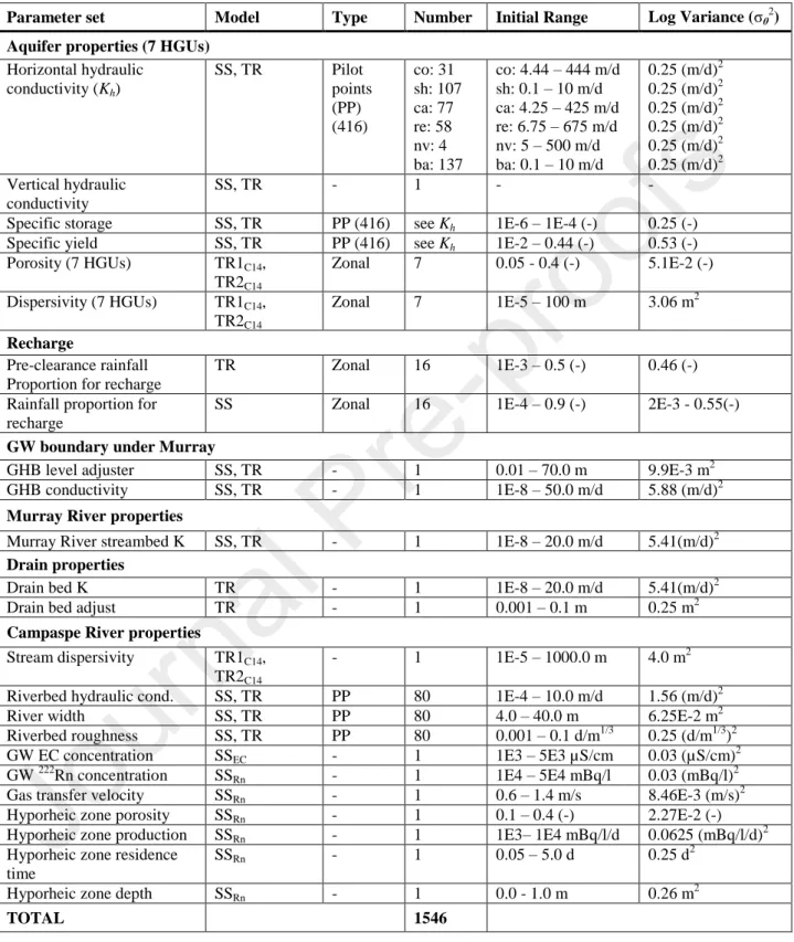
Table 2. Summary of model parameterization. For the aquifer property parameters, the

285

hydrogeological units are abbreviated as follows: Coonambidgal (co), Shepparton (sh),

286

Calivil (ca), Renmark (re), Newer Volcanics (nv), Basement (ba).

287

The flow and transport models were built utilising FloPy (Bakker et al. 2016). The in-288

stream transport model for 222Rn and EC was implemented in Python (see SI). 289

3.2 Assessment of predictive uncertainty in SW-GW exchange flux

290

The worth of data is considered herein as the reduction or lack thereof of the uncertainty 291

of the prediction of interest (SW-GW exchange) with the addition of various acquired or 292

potential observation data. A brief overview of the key theoretical aspects underlying the 293

approach adopted for the quantification of predictive uncertainty and data worth is now provided. 294

The posterior (i.e., post-history matching) parameter covariance matrix ( can be 295

estimated with Schur’s complement as (Christensen and Doherty 2008; Doherty 2015; Tarantola 296

2005; White et al. 2016): 297

(1) 298

Where, is the prior parameter covariance matrix, is the epistemic noise covariance 299

matrix (i.e. accounting for both measurement and model error), and is the Jacobian matrix of 300

partial first derivatives of model outputs (for which there are corresponding observations) with 301

respect to parameters θ. The second term on the RHS of (1) expresses the reduction in 302

uncertainty surrounding parameters as a result of conditioning the model on the information 303

contained in the observations. 304

The prior and posterior uncertainty variance for a prediction s, , respectively can be 305

estimated via uncertainty propagation: 306

(2) 307 And 308 (3) 309

Where is the sensitivity vector for prediction s with respect to the parameters θ (a row 310

extracted from the matrix). 311

This study assumes the parameter covariance matrix ( ) is a diagonal matrix (does not 312

contain non-zero off-diagonal elements). This assumption means that zero correlation exists 313

between parameters. The assumption of zero correlation between spatially distributed 314

parameters, and in particular pilot point aquifer and river property parameters was considered 315

appropriate given the limited spatial coverage of both aquifer and river property information as 316

well as the large distance separating pilot points (on average, 6 km x 6 km). The lower and upper 317

bounds of the parameter range (see Table 2) are specified based on hydrological and geological 318

expert knowledge (in this case conservative) and are assumed to represent the 5th and 95th 319

percentile of the (assumed Gaussian) parameter distribution. 320

The Jacobian matrix was populated using 1% two-point derivative increments. These 321

derivatives with respect to a parameter set were obtained following a history matching 322

undertaking that is unrelated to the implementation of the data worth analyses presented herein 323

(see SI for details). 324

The epistemic noise covariance matrix ( ) is also assumed diagonal. It is specified 325

practically by assigning observation weights (inversely proportional to the standard deviation of 326

noise) (Doherty 2015). Observation weights are specified on the basis of a subjective assessment 327

of the measurement noise standard deviation (Table 3), before being adjusted in accordance with 328

model-to-measurement residuals to account for model error. Weight adjustment is undertaken in 329

such a way that the weight of any observation cannot be increased (thereby respecting the 330

contribution to epistemic noise from measurement noise), and that the contribution of each 331

observation group to the model-to-measurement objective function is equal to the number of 332

non-zero weighted observations in that group (Doherty 2016). The use of model-to-measurement 333

residuals to approximate model error is deemed appropriate given that this quantity can never be 334

known, and that the residuals constitute the only information available for reflecting model error 335

with respect to different types of observation and simulated outputs. For potential observations, 336

i.e., where no measurements exist for which to undertake the above-described weight adjustment, 337

weights are specified based on the average (adjusted) weight assigned to existing observations of 338

the same group/type. The observation noise variance for all but stream flow was fixed as stream 339

flow measurement error is known to become larger at higher flows, particularly when 340

extrapolating the rating curve (Di Baldassarre and Montanari 2009) and an assumed 40% error 341

accounts for a worse case evaluation of this error. The posterior parameter covariance matrix and 342

ensuing data worth analysis was calculated using the Python package pyEMU (White et al. 343

2016). 344

Table 3. Assumed observation noise (used together with model-to-measurement residual

345

information to populate ).

346

The worth of different observation data is evaluated in different ways in this study. 347

Firstly, we consider the worth with observation data groups by themselves, i.e. the ability of an 348

individual observation data group to reduce uncertainty on a prediction of SW-GW exchange. To 349

do this, predictive uncertainty with that particular observation data group is estimated by 350

evaluating equation 1 and 3 twice, once where the particular observation data does not appear in 351

, which we term the ‘base’ uncertainty ( ), and again where contains the particular

352

observation data group, which gives the ‘group’ predictive uncertainty ( . The 353

calculation of reduction in uncertainty through adding the observation data type group (DWadd%)

354 is calculated as: 355 (4) 356

Secondly, to evaluate the mutually exclusive information that exists in each observation 357

data group we consider the difference between predictive uncertainty reduction using all 358

observation data groups and omitting an observation data group from all groups. To do this, we 359

again evaluate equation 1 and 3 twice, once where in all observation data groups are 360

considered together ( ), and again with all observation data groups except for the one of 361

interest considered ( ). Then we compare the two against the ‘base’ uncertainty:

362

(5)

363

Finally, in the context of the potential observations, we evaluate the next most important 364

observations (using built in functions in pyEMU; White et al. (2016)) by iterating over each of 365

the potential observations alone (for select predictions) and in groups (for all predictions within a 366

group) to find the best reduction in uncertainty, then we add that observation or group of 367

observations to the list of existing observations and repeat the process. The addition of the 368

previously identified best observation or observation group accounts for any correlation between 369

observations or groups of observations. 370

In order to answer the first question posed (Q1) regarding the degree to which water 371

chemistry data and hydraulic data reduces the uncertainty surrounding the 156 predictions of 372

SW-GW exchange, each of the observation data types (or “groups”) were first considered 373

individually for existing observation data with the “base” containing no observation data (Table 374

4). Then the potential data (Q2) were evaluated with the “base” consisting of all existing 375

observation data. The individual contribution of each potential observation to the whole of river 376

exchange at three different times covering low, regular and high streamflow conditions was 377

examined to determine the worth of particular potential data types and quantities of value. 378

Table 4. Data worth assessments employed for the range of SW-GW exchange predictions

379

from the Campaspe transient flow model (TR).

380

4 Results and Discussion

381

4.1 Simulated SW-GW exchange behaviour

382

The behaviour of SW-GW exchange flux is first examined at each of the TR model’s 122 383

stream segments on a monthly basis as a means of establishing an understanding of dynamics 384

and spatiotemporal variability of the exchanges before considering the data worth analysis. 385

Throughout the results section we adopt the convention of denoting gaining conditions in 386

a stream by negative values and losing conditions by positive values. The monthly flows are 387

herein subjectively categorised as either low (<35th percentile), regular (between 35th and 80th 388

percentile), or high (>80th percentile). Each of the flow categorisations is also associated with 389

clearly differing SW-GW exchange patterns. 390

The post-clearance transient flow simulation generally showed that SW-GW exchanges 391

along the length of the river exhibit gaining behaviour (Figure 4). The exception to this being 392

during high flow events, when the river transitions to a largely losing river (0.23 m2/d) as 393

significant inflows from Lake Eppalock raise the stream stage and reverse the hydraulic gradient 394

along the majority of the river. The exchange fluxes per unit length of stream at any point along 395

the stream during the simulation period range from losing by 9 m2/d during the October 2016 396

high flow event to gaining at -9 m2/d as the system recovers in the following month. The 397

spatially and temporally averaged SW-GW exchange along the entire river is gaining at 398

approximately -1.1 m2/d. Reach r3 shows the strongest variance in exchange flux along its length 399

through differing inflow conditions followed by r5, r6 and r8, while r10 and r11 show the least 400

variance and are always gaining. 401

402

Figure 4. Simulated SW-GW exchange fluxes per unit length of stream at each reach along

403

the Campaspe River. Coloured lines depict exchange fluxes under differing low, regular or

404

high flow conditions for each month. The black line depicts the temporally averaged

405

exchange flux. The dotted grey vertical lines indicate gauge locations with the 11

between-406

gauges-reaches annotated at the top of the graph.

407

The simulated SW-GW exchange fluxes for the whole river and for each of the 11 river 408

reaches for annual average and monthly average time scales (i.e. 156 predictions) range from -409

3.08 to 2.23 m2/d (shown in Figure 5). The strongest losing flux appears along reach 3 during the 410

high flow event in October 2016. The simulated SW-GW exchange flux was highest along reach 411

3. Reach 6 (r6) just upstream of the Campaspe weir exhibits losing conditions, while all other 412

reaches show gaining conditions. For the examined year, there is a clear link between the inflow 413

from Lake Eppalock and the pattern of exchange fluxes (Figure 5). 414

415

Figure 5. Heatmap of simulated SW-GW exchange per unit length along the whole of the

416

river and along each of the 11 reaches at annual and monthly time scales, which comprises

the 156 predictions of interest. Red cells in the heatmap indicate losing conditions and blue

418

cells indicate gaining conditions. The left panel shows the location and length of each of the

419

reaches for reference. The bottom panel indicates the annual average (mean) inflow from

420

Lake Eppalock to the system as well as the monthly inflow with the colours of the bars

421

indicating whether the flow is low, regular or high.

422

4.2 Worth of existing hydraulic and water chemistry data types (Q1)

423

Assessment of the worth of individual observational data types alone (i.e., DWadd%) for

424

the spatial and temporally aggregated whole of river annual exchange showed that hydraulic 425

head followed by EC, 222Rn and flow observation groups had sizeable worth of > 40% (the green 426

dots in Figure 6a). Similar relative trends across data types were seen for the uncertainty 427

increases without individual data groups when compared to all data groups (DWremove%). The

428

lower values in DWremove% as compared to DWadd% arise because the former yields the unique

429

information contained in an individual data group; this allows for assessment of the extent of 430

correlation and redundancy of individual data groups. It was evident from the analysis of 431

DWremove% for the spatially and temporally averaged SW-GW exchange prediction, that the head, 432

streamflow, 222Rn and EC data contain unique information. 433

Across all 156 predictions for SW-GW exchange flux predictions along the Campaspe 434

River, the median worth obtained from both DWadd% and DWremove% showed that head data were

435

significant whereas the streamflow data were less informative. Furthermore, there appears to be 436

redundancy in the flow data. Also, the median worth of 222Rn was significant whereas the EC 437

data was much lower (Figure 6a). Stream stage and 14C were both poor, with the distribution of 438

DWadd% for stream stage data close to zero. The large range in worth of head, flow, 222Rn and

439

EC data types and the degree of information redundancy across the 156 predictions highlights the 440

nature of the local information content that particular data types have for specific predictions. 441

The local information content is highlighted by the outliers in DWremove% showing unique

442

information in head, 14C and 222Rn for some predictions of SW-GW exchange. 443

Figure 6. Analysis of worth for the whole of river annual exchange (green dots) shown by a)

444

% reduction in predictive uncertainty for SW-GW exchange associated with each

445

particular observation group (DWadd%), and b) difference in reduction between using all 446

observation data types and using all except for a particular group from the combination

447

(DWremove%). Furthermore, boxplots are shown for the distributions across all 156 SW-448

GW exchange predictions.

449

The worth for the 156 SW-GW exchange predictions shows distinct patterns that are 450

associated with inflow to the Campaspe River from Lake Eppalock (Figure 7). During the large 451

flow event during October 2016, across all reaches and the whole river there was consistently 452

poorer worth for predictions within that month. The relative lack of information resident in the 453

data types continues in the following months associated predictions, while the system recovers. 454

The whole of river predictions show an expected dampened variability and higher average worth 455

due to its spatially integrated nature. At the end of the river system in reaches r10 and r11 all data 456

types are seen to have quite low worth, except 222Rn which appears to be the only data-type to 457

show value in reach r10. The poor performance at the end of system could be due to a “boundary 458

effect”, related to the fact that both the Murray River boundary condition and underlying 459

groundwater general head boundary conditions possibly influence the model to such an extent 460

that they overpower the information content of any existing observational data. Potential 461

boundary effects could be avoided by extending the northern boundary of the model past the 462

Murray River and converting the Murray River to a flow routing representation rather than the 463

fixed head representation that was implemented. 464

Figure 7. Heatmaps of percentage reduction in SW-GW exchange uncertainty obtained

465

with all data (a), and with each of the observation data types alone (b-g). The reduction is

466

shown for each SW-GW exchange flux considered, i.e. for each of the stream reaches

(r1-467

r11) and whole of river (nrf), and at each of the temporal scales of annual and monthly

468

between the start of June 2016 and end of May 2017. The inflow to the system is shown

469

under the first heatmap (a) from which the high flow event in October can be seen. The

470

locations and lengths of reaches (r1-r11) are shown to the left of the first heatmap for

471

reference.

472

The analysis of existing observation data types, firstly, identified that the temporal 473

integration in annual predictions (both whole of river and reach scale) generally led to better 474

reductions in uncertainty than in the monthly predictions. These are plausible given that the 475

annual signal is smoothed. For hydraulic head, 14C and 222Rn, there were not data available in 476

every month of the year, but particular data were at least present enough in the seemingly 477

dependent months (during large exchanges) required to inform the annual SW-GW exchange 478

prediction. 479

4.3 Worth of individual potential future hydraulic and water chemistry data points (Q2)

480

We analysed the worth from individual potential in-stream observations to explore the 481

extent to which the whole of river SW-GW exchange prediction reliability could be improved 482

through data acquisition at new sampling locations. The worth of individual potential 483

observations of stage, flow, 222Rn and EC at select times when flow conditions were low (July 484

2016), high (October 2016) and regular (November 2016) are shown in Figure 8; the 485

corresponding SW-GW exchange along the stream at each of these times is also shown. The 486

value of both stage and EC potential observations are shown to be poor across these flow 487

conditions, with only 222Rn (low and regular flow conditions) and flow (high and regular flow 488

conditions) showing considerable value. Under low flow conditions, 222Rn data displayed the 489

highest utility where existing data were not present and where the stream exhibits strong gaining 490

conditions in the first 40 km of the stream. Also, 222Rn showed considerable value in the slightly 491

gaining areas at around 130 km downstream, likely due to the paucity in local existing data for 492

all data types. However, 222Rn data were seen to be of low utility when high flow conditions 493

prevail with a corresponding reversal of hydraulic gradient resulting in a mostly losing river, as 494

simulated during the high flow event in October 2016. In the high flow event instance, there is a 495

trend of increasing flow data worth with distance downstream. 496

497

Figure 8. Further reduction in uncertainty for net SW-GW exchange in October 2016,

498

November 2016 and May 2017 obtained through potential observations of stream stage,

499

flow, 222Rn and EC at 80 locations along the stream. Each potential observation is

500

considered alone but added to the existing observations across all observation data types.

501

Underlying each uncertainty reduction plot is the pattern of exchange along the river

502

during each of the months with the scatter showing the exchange rate (m2/d) and the

503

colours representing the exchange flux along the reach at that location; reds indicate losing

504

and blues indicate gaining conditions. The mean exchange rate is shown in light grey on

505

each of these plots to give context to the exchange conditions relative to the mean.

To explore the extent of reduction in uncertainty obtained through potential addition of 507

subsurface data to the existing dataset, we analysed the whole of river SW-GW exchange flux 508

during low, high and regular flow conditions through both head and 14C in the shallow and deep 509

aquifers at the potential sampling locations (Figure 9). The SW-GW exchange along the 510

Campaspe River in the highest (southern) parts of the model domain is very sensitive to the GW 511

level which is strongly connected at the top of the catchment to the heads in the narrow alluvial 512

channels and hence it is observational data located here that appears to inform the whole of river 513

SW-GW exchanges the most, although the reductions in predictive uncertainty are only 514

marginal. This generally highlights opportunity for more value from targeted observations in the 515

southern part of the catchment in the narrow alluvial valleys. The deep heads are seen to hold the 516

least value of the potential observations across flow conditions. As expected, due to the lesser 517

variance of subsurface data as compared to stream data, spatial patterns of worth are more 518

consistent across the low, regular and high flow conditions. Furthermore, there is clear crossover 519

of high utility potential sampling locations for shallow and deep 14C and shallow head too in the 520

southern part of the catchment, although shallow head also appears of some value along the 521

entire length of the stream. 522

523

Figure 9. Percent reduction in uncertainty for annual whole of river SW-GW exchange

524

fluxes of the Campaspe River obtained through hydraulic head and 14C at potential

525

sampling locations (identical to pilot points) in the shallow and deep aquifers.

526

4.4 Worth of potential future hydraulic and water chemistry data types (Q2)

527

For all of the potential data and also each of the data type groups, we examined the 528

benefit of using all potential data (Figure 10), which highlights the extent to which particular 529

predictions can be improved (as compared to existing data) under comprehensive sampling of all 530

data types and individual data types. The potential hydraulic head data showed improvement in 531

terms of SW-GW prediction reliability in the middle section of the river prior to the largest of the 532

high-flow events and a few months after the recovery of this event (Figure 10b). The stage data 533

again shows little value, no matter the location or time of sampling (Figure 10c). The ubiquitous 534

poor worth of stage data was surprising as it could be assumed that the intrinsic link between 535

hydraulic head and stage in the calculation of the exchange flux would result in stage data 536

containing prediction-relevant information. We posit a potential reason for this is the stream 537

stage as simulated by the numerical model showed less variance (minimum and maximum of 538

1.21E-4 and 1.11E-2) then the observed data owing to the representation of a rectangular channel 539

and associated parameterisation. For example, the effective stream width may have been 540

overestimated in the model and hence the associated error with the simulated stage was 541

potentially overrated. This led to a poor rating in stage data but is likely more linked to the 542

modelling assumptions, e.g. a perfectly known riverbed elevation, and structure for the 543

Campaspe River, rather than the “true” worth of the data itself. 544

Further reductions in predictive uncertainty up to around 25% are seen with the addition 545

of the flow, head and EC data. The addition of potential 222Rn data (Figure 10f) shows clear 546

improvements for reaches r2–r9. Especially of interest are those improvements in worth at the 547

time prior to the high flow in October 2016 and just after. Assessment of potential 14C data 548

showed significant improvement of a further 40% reduction in most predictions along reaches 549

r1–r5 (Figure 10e), suggesting that the existing spatiotemporal 14C data locations were 550

suboptimal in this context of SW-GW exchange. However, the comprehensive sampling of both 551

222

Rn and 14C through space and time is likely impractical due to the costs, especially for 14C 552

which would incur drilling costs. 553

Figure 10. Difference in uncertainty reductions between existing and potential observation

554

data for all data (a) and for each of the individual observation groups (b-g).

555

The analysis of the ten “next best” most important observations to collect on top of all 556

existing data during low, high and regular streamflow conditions showed that the optimal 557

location set is different under differing flow conditions. 222Rn was the most beneficial data type 558

to collect next with head, 14C, and flow also in the top ten (Figure 11). Interestingly, during low 559

and high streamflow conditions, within-stream observations of 222Rn and flow were distributed 560

in the upper, middle and lower reaches of the stream, whereas for regular flow conditions, the 561

observation data were in the middle and lower reaches only. The role of 14C observations in the 562

top left of the maps (Figure 11a-c) are at first perhaps counter-intuitive, however, this location 563

represents the longest flow path through the aquifers before exiting through the northern 564

boundary, informing the velocity of flow and its variation and hence the hydraulic conductivity 565

of the aquifers and its effective porosity, the former of which in turn informs the SW-GW 566

exchange along the river. 567

Figure 11. Locations and rank of 10 next most important potential observations to add to

568

the existing observations for whole of river exchange during months of low, high and

569

regular streamflow conditions (a-c). Further reduction in uncertainty (%) due to each of

570

the 10 next most important potential observations (d-f).

571

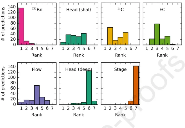
Finally, we examined the next most important observation groups for each of the 156 572

SW-GW exchange predictions (Figure 12), i.e. using all potential data within each data type. 573

This assessment showed that potential 222Rn was the most important group across the majority of 574

predictions, followed by shallow head, 14C, EC, flow, deep head and lastly stage, which was 575

ranked 7th for the majority of predictions (Figure 12). 576

Figure 12. Ranking (x-axis) of best uncertainty reduction across each of the 156 predictions

577

of interest in a “next most important” type analysis. The uncertainty reduction is based on

578

each observation group for potential observations when added to the existing data.

579

4.5 General observations

580

The above results have demonstrated that the worth of different hydraulic and chemical 581

observations in the context of making SW-GW predictions is dependent on the prevailing 582

streamflow conditions, the magnitude and direction of the SW-GW exchange and the spatial and 583

temporal scale of the exchange considered. It has also demonstrated the large variability in worth 584

across different SW-GW exchange predictions as a result of these dependencies. These findings 585

are in addition to previously reported dependence of data worth on prediction specificity more 586

generally (e.g. Dausman et al. 2010; White et al. 2016). 587

4.5.1 Influence of streamflow conditions and magnitude and direction of SW-GW exchange 588

The prediction-specificity of data worth with respect to prevailing stream flow conditions 589

can be explained by the sensitivities of the different SW-GW exchange predictions to uncertain 590

model parameters that are conditioned on the basis of both existing and potential hydraulic and 591

chemical observational data. During high-flow conditions, generally lower data worth is 592

apparent. This is because SW-GW exchange predictions under high-flow conditions depend on a 593

larger portion of uncertain model parameters (e.g., recharge and aquifer properties for the TR 594

model); this results in lower worth given the limit on the ability of information to “spread” from 595

data in space and time. That is, there are a number of prediction-parameter sensitivities that are 596

heightened as the Campaspe flow system is perturbed firstly by large losing SW-GW exchanges, 597

and secondly by the presence of distributed above-average recharge which also propagates 598

through the subsurface. Furthermore, the uncertainty in the flow observations increases with high 599

flows. As the stream is largely losing during high flows, the SSEC and SSRn transport parameters

600

become less sensitive with respect to the corresponding SW-GW predictions. During low-flow 601

conditions, where rainfall recharge is often relatively small and the river is generally weakly 602

gaining along the Campaspe River, the SW-GW exchange predictions are generally less sensitive 603

to the flow model parameters. This allows for the information contained in the 222Rn and EC 604

observations to be used more effectively through the SSEC and SSRn transport parameters.

605

For example, in the annual whole of river SW-GW exchange flux prediction, it was 606

apparent (Figure 8) that in-stream sampling of 222Rn can lead to a further reduction in uncertainty 607

(up to 10%) during low flows, with some value during regular flow conditions (up to 6%) but 608

with reduced utility (<0.5%) in high streamflow conditions. This is because the predictions 609

during lower flow show higher sensitivity to the parameters that are conditioned by the 610

information contained in the 222Rn observations. It is thus necessary to target the particular time 611

and location carefully for sampling water chemistry data due to the transient and local 612

information content. This is further evidenced by the improvements through all potential data for 613

each data type which showed the theoretically possible improvements when comprehensive 614

sampling takes place in space and time. This differs in comparison to the hydraulic data, which 615

seems to show similar patterns across sampling times in worth for groundwater hydraulic head 616

and streamflow data points as explained above (Figure 8 and Figure 9). Despite the similar 617

patterns, the “flow of information” from hydraulic observation data appears to be larger under 618

regular and high flow conditions. 619

As was explained at the start of the results (4.1), the general patterns between flow 620

conditions and SW-GW exchange are clear. The apparent information content in all observation 621

data appears linked to the magnitude and direction of the SW-GW exchange flux in many 622

predictions. It was evident that for the very weakest exchanges, the poorest worth was found, no 623

matter the data type; however, the opposite was not true for the strongest SW-GW exchanges 624

which exhibit more complex worth patterns across data type. 625

4.5.2 Influence of spatial and temporal scale of SW-GW exchange 626

The simulated variability in monthly reach-scale SW-GW exchange in the Campaspe 627

River was clear, and so were the corresponding reductions in predictive uncertainty due to data 628

collection. When averaging the SW-GW exchange over the whole of the river, the worth of data 629

was reasonably consistent on a monthly basis for each data type alone and for all data types, with 630

a clear trend in variability being linked to the flow conditions (discussed above). Furthermore, 631

the consistent data worth across months was also consistently close to the best uncertainty 632

reductions from the reaches, i.e. the reductions were not a simple average of the individual reach 633

uncertainty reductions, but more closely linked to the best reductions. This is expected due to the 634

spatial integration of information contained in the hydraulic and chemical data. A similar pattern 635

with respect to temporal integration of information is present in comparing monthly to annual 636

SW-GW exchanges. 637

There was no clear relationship between the length of the reach and annual reductions in 638

predictive uncertainty. However, the lowest uncertainty reductions were apparent in the shortest 639

reach r10 (0.8 km). The lack of a clear relationship is likely due to a combination of the above-640

mentioned factors of prevailing flow conditions and magnitude of the SW-GW exchange fluxes. 641

4.5.3 Model simplifications and assumptions 642

Interestingly, even though the water chemistry data provide more indirect means to 643

calculate SW-GW exchange flux than the hydraulic data (i.e., chemistry data serve as proxy for 644

flux), these data types alone showed greater worth in many predictions. For the cases in which 645

the river is not experiencing low-flow conditions and gaining, we would posit that this is partly a 646

result of the simplified 1D transport models (SSRn and SSEC) used to map the 222Rn and EC

647

observations to SW-GW exchange predictions through the SSRn and SSEC transport parameters.

648

The parameterisation, spatial scale of river segments, and process assumptions that were applied 649

to the simplified 1D transport model (e.g., the uniform fixed groundwater concentrations of 222Rn 650

and EC, and the monthly steady-state assumption) likely inflates their sensitivity for these data 651

types and hence their worth to SW-GW exchange predictions (Fienen et al. 2010). Future 652

modelling of in-stream 222Rn and EC transport would benefit from testing this by further 653

evaluating the worth of these data types in a transient transport model with spatiotemporally 654

varying parameters, including the inputs of both 222Rn and EC. With appropriate data collection 655

of times series data of near-stream GW 222Rn and EC, future modelling of the Campaspe system 656

may benefit from explicit modelling of groundwater transport of 222Rn and EC to help 657

demonstrate that current the boundary simplification of 222Rn and EC to static GW conditions 658

does not introduce large impacts to the data worth analysis. 659

The simulation of SW-GW exchange is of course subject to some simplifying 660

assumptions that were employed to develop a tractable regional-scale model of the Campaspe 661

system for the data worth analysis. Such simplifications include, but are not limited to, that of 662

ignoring unsaturated zone flow processes, ignoring representation of overland flow during 663

flooding and mostly non-contributing small tributaries, and the exclusion of a hyper-resolution 664

model grid for solving the governing equations. For example, in the case of ignoring unsaturated 665

flow, it has been shown previously by Brunner et al. (2010) that the violation of the assumption 666

of a hydraulically connected losing-gaining system will lead to underestimation of infiltration of 667

GW. More generally, model simplifications (e.g., 1D steady-state transport, surface flow 668

representation, ignoring unsaturated flow processes, numerical discretization errors, etc.) are 669

likely to lead to uncertainty variance under-estimation (e.g., Knowling et al. 2019b; White et al. 670

2014); however, our relativistic (i.e., concerning changes in second moments) analysis of worth 671

is expected to be somewhat immune to the impact of such model simplifications. As the 672

Campaspe system becomes better characterised in the future and the model employed herein is 673

refined, exploration of such simplifications could potentially benefit the interpretation of worth. 674

4.5.4 Choice of data types 675

This study focused on the worth of particular observational data in the context of SW-676

GW exchange. It was not exhaustive of all possible data types, and didn’t include, e.g. other 677

stream chemistry data, such as stream 14C, dissolved organic carbon (DOC) or total inorganic 678

carbon (TIC), due to the complexity of additional carbon processes required to model these. It is 679

recognised that, e.g., hydrometeorological data such as evapotranspiration and precipitation data, 680

physical stream property measurements, aquifer property measurements and data informing the 681

3D hydrostratigraphic model including its geometry and internal facies distribution may also be 682

of worth and warrant investigation in future studies. 683