A large paleoearthquake in the central Apennines, Italy, recorded by the collapse of a cave speleothem

HAL Id: hal-03106691

https://hal.archives-ouvertes.fr/hal-03106691

Submitted on 19 Apr 2021

HAL is a multi-disciplinary open access

archive for the deposit and dissemination of

sci-entific research documents, whether they are

pub-lished or not. The documents may come from

teaching and research institutions in France or

abroad, or from public or private research centers.

L’archive ouverte pluridisciplinaire HAL, est

destinée au dépôt et à la diffusion de documents

scientifiques de niveau recherche, publiés ou non,

émanant des établissements d’enseignement et de

recherche français ou étrangers, des laboratoires

publics ou privés.

Bruno Pace, Alessandro Valentini, Luigi Ferranti, Marcello Vasta, Maurizio

Vassallo, Paolo Montagna, Abner Colella, Edwige Pons-Branchu

To cite this version:

Bruno Pace, Alessandro Valentini, Luigi Ferranti, Marcello Vasta, Maurizio Vassallo, et al.. A large

paleoearthquake in the central Apennines, Italy, recorded by the collapse of a cave speleothem.

Tec-tonics, American Geophysical Union (AGU), 2020, 39 (10), �10.1029/2020TC006289�. �hal-03106691�

Bruno Pace1,2 , Alessandro Valentini1, Luigi Ferranti3,2, Marcello Vasta4, Maurizio Vassallo5 , Paolo Montagna6, Abner Colella3, and Edwige Pons‐Branchu7

1_{DISPUTER—Università degli studi Gabriele d'Annunzio, Chieti, Italy,}2_{CRUST—Centro inteRUniversitario per l'analisi}

SismoTettonica tridimensionale con applicazioni territoriali, Chieti, Italy,3_{DiSTAR—Dipartimento di Scienze della}

Terra, dell'Ambiente e delle Risorse, Università di Napoli“Federico II”, Naples, Italy,4INGEO—Università degli studi Gabriele d'Annunzio, Chieti, Italy,5_{Istituto Nazionale di Geofisica e Vulcanologia, sezione di Roma1, sede di L'Aquila,}

L'Aquila, Italy,6Institute of Polar Sciences, ISMAR‐CNR, Bologna, Italy,7Laboratoire des Sciences du Climat et de l'Environnement, LSCE/IPSL, CEA‐CNRS‐UVSQ, Université Paris‐Saclay, Gif‐sur‐Yvette, France

Abstract

Speleoseismological research carried out in the Central Apennines (Italy) contributed to understanding the behavior of active normal faults that are potentially able to generate Mw6.5–7

earthquakes documented by paleoseismology and by historical and instrumental seismology. Radiometric (U‐Th, AMS‐14C, and bulk‐14C) dating of predeformation and postdeformation layers from collapsed speleothems found in Cola Cave indicates that at least three speleoseismic events occurred in the cave during the last ~12.5 ka and were ostensibly caused by seismic slip on one or more of the active faults located in the region surrounding the cave. We modeled the collapse of a tall (173 cm high) stalagmite tofind a causative association of this event with one among the potential seismogenic sources. We defined the uniform hazard spectrum (UHS) for each seismogenic source at the site, and we used the calculated spectra in a deterministic approach to study the behavior of the speleothem, through a numericalfinite element modeling (FEM). Although our analysis suggests the “Liri” fault as the most likely source responsible for the ground shaking recorded in the cave, the“Fucino” fault system, responsible for a Mw7 earthquake in 1915, cannot be excluded as a potential source of

speleoseismic damage. Results of this work provide new constraints on the seismotectonic history of this sector of Central Apennines and highlight the performance of integrated speleoseismological, seismic hazard, and numerical studies.

1. Introduction

Cave speleothems can be used not only for paleoenvironmental and paleoclimatic reconstructions (Bar‐Matthews et al., 1999; Gascoyne et al., 1980; Lauritzen, 1995; Li et al., 1989; McDermott, 2004; Talma & Vogel, 1992) but also for speleoseismological research, that is, the investigation of traces of ancient earth-quakes in caves (Becker et al., 2006; Kagan et al., 2005). Since the 80's, researchers (e.g., Forti, 2001; Forti et al., 1981; Forti & Postpischl, 1980, 1984; Postpischl et al., 1991; Rajendran et al., 2016) established that in the proved absence of other deformation sources (landslide,flooding, ice flow, animal, or anthropic passage), the deviation of the growth axis from the vertical and the speleothem collapse are evidence for seismic shaking of cave walls. Improvements in analytical techniques and theoretical modeling also showed that in earthquake‐prone regions, unbroken speleothems that have survived all the earthquakes occurred during their life span may provide constraints on seismic hazard estimates, allowing to extend the window of observation of a given historical catalogue (Di Domenica & Pizzi, 2017; Ferranti et al., 2019; Gribovszki et al., 2013, 2018).

In terms of seismic hazard, the main issue concerns the evaluation of the ground motion potentially responsible (or not) of the speleothems collapse. Cadorin et al. (2001) carried out laboratory measure-ments on stalagmite samples to study their failure in bending and estimate the ground acceleration neces-sary to break speleothems. Similarly, Lacave et al. (2000, 2004) investigated the mechanical behavior of speleothems via static bending tests and estimated the probability that at least one moderate earthquake has occurred in the past. Recently, Mendecki and Szczygieł (2019) provided quantitative relationships between speleothems shape and their oscillation and acceleration during shaking. In these studies, the

©2020. American Geophysical Union. All Rights Reserved.

Key Point:

• Performance of integrated speleoseismological, seismic hazard and numerical studies

Correspondence to:

B. Pace,

bruno.pace@unich.it

Citation:

Pace, B., Valentini, A., Ferranti, L., Vasta, M., Vassallo, M., Montagna, P., et al. (2020). A large paleoearthquake in the Central Apennines, Italy, recorded by the collapse of a cave speleothem. Tectonics, 39, e2020TC006289. https:// doi.org/10.1029/2020TC006289

Received 5 MAY 2020 Accepted 29 AUG 2020

underlying idea is based on the stalactite‐stalagmite oscillatory system, which represents the vertical datum. However, the difficulty in quantitative modeling of the observed deformation and its direct attribution to a seismogenic source remains a major issue (Becker et al., 2006; Ferranti et al., 2019; Lacave et al., 2004).

The aim of the present work is to reconstruct the speleoseismological history of Cola Cave (Abruzzo region, Central Italy, Figure 1) and to investigate the causes that led to the collapse of a tall (173 cm high) spe-leothem found in the cave. We were motivated to establishing whether this collapse represents the record of a large paleoearthquake and how this and other speleoseismic event that we found in the cave are framed in the seismotectonic context of the Central Apennines.

Cola Cave is located in the internal sector of the Central Apennines (Figure 1), an area presently affected by NE‐SW trending geodetic extension at 2 and 3 mm/yr (Cheloni et al., 2017; D'Agostino, 2014; Devoti et al., 2011). Extension is accommodated by systems of NW‐SE striking normal faults (Figure 1; Boncio et al., 2004; Pace et al., 2006; Valentini et al., 2017). The present activity of most Central Apennines faults is constrained by several evidence, and a number of them are considered seismogenic sources potentially able to generate Mw6.5–7 earthquakes (DISS Working Group, 2015; Pace et al., 2006, 2010; Verdecchia

et al., 2018) documented in the Central Apennines (Figure 1; Boncio et al., 2004; Chiaraluce et al., 2011; Galli et al., 2008).

Although a good age record exists for Late Pleistocene–Holocene earthquake slips from fault scarp analysis (e.g., Galadini & Galli, 2000; Roberts & Michetti, 2004; Schlagenhauf et al., 2011), and trench paleoseismol-ogy (e.g., Cinti et al., 2011; Galli et al., 2008) on the major Central Apennines faults, there are still contrasting views about the capability of several faults to generate earthquakes.

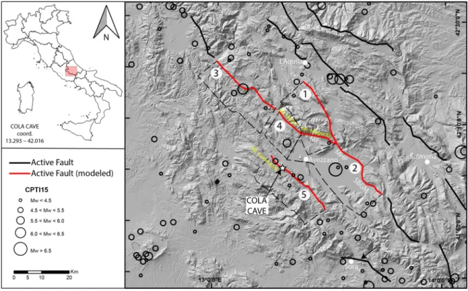
Figure 1. Tectonic sketch of the studied area. The star represents the Cola Cave (coordinates in the box); the black circles represents the epicenters of the historical earthquakes reported in the CPTI15 catalogue (Rovida et al., 2016); the black lines are the major active faults outcropping in the area (in red the active faults modeled in this work). The numbers represent the modeled seismogenic sources: 1:“Campo Felice‐Ovindoli”; 2: “Fucino”; 3: “Salto Valley”; 4: “Velino”; 5: “Liri”. MF: Magnola fault; MHP: Marsicano Highway‐Parasano fault; SBGM: San Benedetto‐Gioia dei Marsi fault. The hillshade has been produced from a DEM available at: http://www.sinanet.isprambiente.it/it/sia-ispra/download-mais/dem20/view.

2. Seismotectonic Context

Cola Cave is surrounded by major active faults, and the region has been shaken by large earthquakes; the lar-gest of them occurred over the last century (Fucino 1915 Mw7; L'Aquila 2006 Mw6.3; Central Italy 2016

Mw6.5). The active faults are mainly south west‐dipping normal faults and are organized in fault systems.

Some of them are considered seismogenic (Boncio et al., 2004; Valentini et al., 2017) (red traces in Figure 1). The most important fault system is the“Fucino” (source n. 2 in Figure 1), whose activity controlled the growth of the largest intermontane basin in the Central Apennines during the last ~2 and 3 Ma. The ~38 km‐long surface expression of the Fucino fault system (Galadini & Galli, 1999) is represented, from north to south, by three main fault segments, namely, the Magnola fault (MF, Figure 1), the Marsicana Highway‐Parasano fault (MHP, Figure 1), and the San Benedetto dei Marsi‐Gioia dei Marsi fault (SBGM, Figure 1) (e.g., Giraudi, 1988; Messina, 1996; Michetti et al., 1996; Serva et al., 1986). The 1915 earthquake activated most of the Fucino source producing coseismic ground displacements up to about 1 m high, as described by Oddone (1915) and confirmed by paleoseismological studies (Galadini et al., 1997; Galadini & Galli, 1999; Michetti et al., 1996; Serva et al., 1986). The paleoseismic trenches revealed at least seven addi-tional surface rupture events during the last ~20 ka with offsets comparable to the 1915 earthquake slip (Galli et al., 2008). Galli et al. (2012) found trench evidence of recent activity of the MF segment, with one or more faulting events that have affected the Neoglacial colluvia (post 4.5 ka) before Roman age (~2 ka) deposits. The time span of this event roughly matches the 3.4 ± 0.3 ka age of the penultimate exhumation event found on the fault scarp using the cosmogenic36Cl method (Schlagenhauf et al., 2010).

The“Velino” seismogenic source (source n. 4 in Figure 1) is located north of the Fucino basin and is repre-sented by a bedrock scarp along the southern slope of Mt. Velino. The fault is considered currently active (Boncio et al., 2004; Bosi, 1975) as evidenced by geomorphological and paleoseismological observations (Giraudi, 1992; Pace et al., 2008). Schlagenhauf et al. (2011) carried out cosmogenic36Cl dating of carbonate samples from the exhumed fault plane, reconstructing the slip history over the last 7.5 ka. They recognized five exhumation events with the last occurred around 1.3 ± 0.3 ka. A single earthquake is assigned to the structure in the historical catalogue (CPTI15; Rovida et al., 2016, 2020), the event of 24/02/1904 (I0

VIII‐IX MCS; Mw5.7).

The“Salto Valley” fault (source n. 3 in Figure 1) is a nearly 28 km long structure bordering the north‐east side of the Salto Valley. Some authors believe that the fault is currently active (Papanikolaou et al., 2005; Roberts & Michetti, 2004) on the basis of morphological indications, while according to others, fault activity ended at the beginning of the middle Pleistocene (Galadini & Messina, 2001).

The“Campo Felice‐Ovindoli” fault system (source n. 1 in Figure 1) is characterized by several segments that form a single seismogenic source. The recent activity of the fault system is supported by paleoseismological studies realized on the different segments (e.g., Pantosti et al., 1996; Salvi et al., 2003). Three events that dis-placed Holocene deposits with a recurrence interval of about 3,000 years were identified on the southern seg-ment. The last event occurred in a time interval between 700 and 1,130 years BP (Pantosti et al., 1996). Moreover, the event of 9 September 1349 (Mw6.3, Rovida et al., 2016) has been attributed to the“Campo

Felice‐Ovindoli” seismogenic source activity (Pace et al., 2006).

Finally, the Cola Cave is localized exactly along the ~60 km long“Liri” fault system. While the southern seg-ment (Sora fault, about 20 km long) shows possible signs of seismic activity (Val Roveto earthquake, 1922, Mw5.2), the activity of the central‐northern sector (about 40 km long, source n. 5 in Figure 1) is still a matter

of debate. Galadini and Messina (2004) consider the fault inactive, because of the lack of clear displacement of late Quaternary deposits and suggest that slip occurred during the late Pliocene‐Middle Pleistocene. Roberts and Michetti (2004) studied the along strike variation of vertical dislocation and escarpment height of the fault. Assuming that these two parameters are congruous with the values measured on other active faults in central Apennines, they concluded that exposure of the fault surface is due to tectonic displacement and not to erosional exhumation.

The choice of Cola Cave, for its strategic position in this complex seismotectonic context, may help to better constrain the paleoseismological record of active faults of the region and to explore the activity of doubtful faults, such as the“Liri” fault, whose contribution to seismic hazard and seismic risk models could neverthe-less be notable (Scotti et al., 2020).

3. Cave Morphology

Cola Cave opens at an elevation of ~1,400 m a.s.l. on the south‐west side of Mt. Arunzo, a culmination of an ~15 km long ridge belonging to the M.ti Carseolani mountain group. The ~200 m long cave is developed within thick Cretaceous limestone beds that cap a succession of Mesozoic platform carbonates.

A narrow entrance carved along less competent limestone and marly beds (Point A, Figure 2) leads to a large sub‐rectangular (~60 × 30 m), ~5–10 m high room occupied by fallen ceiling blocks which reach dimensions up to a few m3(Point B, Figure 2). A steep (20° average) northwest‐southeast trending slope brings to the more internal part of room B where large speleothems and columns are grown upon ancient rockfalls. Here, the cave turns to follow a northeast‐southwest trend. To the northeast, the cave again bifurcates (Point C, Figure 2). The main branch continues towards northeast across rooms rich of concretions (Point D, Figure 2), whereas a narrower branch detaches to the east and terminates in a circular room with a small ephemeral lake (Point E, Figure 2). To the southwest of the main room, the cave progressively des-cends getting narrower and reaches a series of small rooms decorated by abundant speleothems and pools (Point F, Figure 2). The cave continues deepening to the southwest through tighter passages and shafts, but we did not explore this section further.

4. Material and Methods

The research methodology integrates:

1. Field work in the cave, which includes structural analysis aimed to exclude that the observed speleothem deformation is the result of local nontectonic processes, measurement of the geometry of collapsed speleothems, and collection of samples from fallen and regrown speleothems to constraint events age;

2. Laboratory work, consisting in (230Th/U) and AMS‐14C dating of pre‐event and postevent layers; 3. Seismic hazard analysis to define a seismogenic source model and calculate the expected ground motion

at the site in terms of uniform hazard spectra;

4. Numerical modeling of a selected fallen stalagmite to study the speleothem behavior during the passage of the expected seismic waves and to estimate the possible seismogenic source of the recorded speleoseis-mic event.

Figure 2. Map of the Cola Cave (modified from a map kindly provided by Daniele Berardi) showing the falling azimuth of broken stalagmites (arrows in map gives the trend; rose diagram distribution in inset provides the direction), the location and labels of dated samples and the seismic noise measurement sites (stars).

4.1. Speleothem Sampling and Cave Structural Analysis

We measured the geometry of 29 collapsed speleothems using a tape and sampled by hammer a selection of them for radiometric dating and geo‐mechanical tests. For each measured speleothem, we recorded the length and the average diameter of the fallen section. For stalagmites, we also tried to recognize the standing stump from which the speleothem fall. Commonly, the stump narrows upwards to form a neck of the pre-failure stalagmite. Indeed, when a large earthquake occurs in the vicinity of the cave, the speleothems oscil-late due to the ground motion until its failure tensile stress may be overcome and the speleothem breaks in the weakest part, the neck (Figures 3a and 3b). Because the stalagmite neck is characterized by a change in orientation of C axes of calcite crystals from horizontal at the base to vertical above (P. Forti, personal

Figure 3. Conceptual model showing the process of seismic breaking of the speleothems. (a) An earthquake occurs in the vicinity of the cave and the speleothems oscillate due to the passage of the seismic waves. (b) The speleothem oscillate due to the ground motion until its failure tensile stress is overcome and the speleothem breaks in the weakest part, often where the C axes of calcite crystals could change in orientation from horizontal at the base to vertical above. The speleothems fall down oriented with the mean direction of the seismic waves. (c) After the collapse, new speleothems grow on top of the base and the fallen part of the broken speleothem. Dating the tip of the fallen part (A) and the base of the new speleothems (B) help to constrain the age of the collapse. (d) If the speleothem is not vulnerable enough, instead of collapsing, it could change its growth axis. In this case, the evidences of earthquakes are in the inner structure of it.

communication, 1999), it represents the weakest section and the potential locus of breakage during seismic shaking (Figure 3b; Lacave et al., 2004).

Based on cave topography and on the geomorphological setting (relative ease of access), we cannot exclude in principle that the observed speleothem deformation is the result of nontectonic processes such as water flooding, flow of ice during past glacial stages, and animal or anthropic passage (Becker et al., 2012; Jaillet et al., 2006; Kagan et al., 2005, 2017). All the above processes are expected to produce a random

Figure 4. Speleothem from the Cola Cave: (a) site of the two fallen stalactites COLA‐20 and COLA‐21: in the two small pictures the sample COLA‐20 in details, before the cut (on the right) and after the cut (on the left), in red the sampled layer; (b) site of TRAP‐1 and TRAP‐2 samples: TRAP‐1 is the younger

stalagmite grown upon the fallen stalagmite TRAP‐1; in the small picture the sample TRAP‐1 in details after the cut, in red the sampled youngest layer; (c) COLA‐3 site: COLA‐1 and COLA‐2 are the two small stalagmites grown above the stump left by the collapsed stalagmite COLA‐3; in the small

picture a detail of the sample COLA‐2 after the cut, with the arrow the sampled oldest layer; (d) CRLL sample site: CRLL is a small stalagmite grown upon a large limestone block fallen from the vault of the cave; in the two small pictures the sample CRLL in details, before the cut (on the right) and after the

orientation of fallen speleothems. Conversely, during seismic shaking, it is predicted that speleothems fall to the ground along a direction broadly aligned with the mean direction of the seismic waves (Figure 3b). To disentangle between a tectonic versus a nontectonic origin for the observed collapses, we measured the fall azimuth of 29 stalagmites. The azimuth distribution clusters along the NNW‐SSE direction, with minor petals to the WSW and NNE (Figure 2). The tight azimuthal distribution argues for a tectonic origin, inasmuch it is roughly parallel with the mean strike of the seismogenic sources of the area (Figure 1). Finally, we sampled both the tip of fallen speleothem and in few cases the base of speleothems grown on the top of the collapsed ones to tightly constrain the age of the collapses (Figure 3c). In some cases, if the speleothem is not vulnerable enough, instead of collapsing, it could change its growth axis. In this case, the evidences of earthquakes are in the inner structure of it (Figure 3d). Indeed, the youngest layer of a fallen speleothem and the base of an intact stalagmite grown upon it represent the pre‐event and postevent layers, respectively (Becker et al., 2012; Forti & Postpischl, 1984; Kagan, 2012; Kagan et al., 2005). When the growth of an intact speleothem was not observed above a collapsed speleothem, we only took its youngest, pre‐event layer.

4.2. Radiometric Dating

Field samples were sawed in half to identify the layers for dating. Subsamples were extracted from the cho-sen laminae of stalagmites and stalactites using a dental drill with diamond‐encrusted blades.

Both the U‐series decay (230Th/U) and AMS‐14C dating techniques were used to date nine samples (Figures 2 and 4). The ages offive samples were accurately determined by U/Th at the Laboratoire des Sciences du Climat et de l'Environnement (LSCE) at Gif‐sur‐Yvette, France using a ThermoScientific NeptunePlus

multi-collector inductively coupled plasma‐mass spectrometer following the protocol developed at LSCE (Columbu et al., 2015; Pons‐Branchu et al., 2014). Details of the analytical procedure for U/Th can be found in Ferranti et al. (2019). An initial230Th/232Th activity ratio of 1.50 ± 0.75 (Hellstrom, 2006) was used to correct for the nonradiogenic detrital230Th fraction (Table 1). Four samples were AMS‐14C dated at the

Table 1

Uranium‐Series Measurements of the Speleothem Samples From the Cola Cave

Sample name Lab code 238U (μg/g) 232Th (ng/g) δ234U_m (230Th/232Th) (230Th/238U) Age (ka) Corrected age (ka BP)a

TRAP 1 6563 0.2756 ± 0.0003 0.402 ± 0.0004 19.855 ± 1.0 31.1 ± 0.5 0.01505 ± 0.0003 1.62 ± 0.03 1.55 ± 0.07

TRAP 2 6564 0.1463 ± 0.0001 0.176 ± 0.0002 16.784 ± 0.8 182.2 ± 1.3 0.07245 ± 0.0005 8.07 ± 0.06 8.01 ± 0.10

COLA 3 6568 0.1418 ± 0.0018 19.482 ± 0.0229 17.307 ± 0.8 3.4 ± 0.0 0.15326 ± 0.0008 17.82 ± 0.11 10.84 ± 3.52

COLA 20 6569 0.2371 ± 0.0005 1.533 ± 0.0014 4.698 ± 0.9 34.9 ± 0.2 0.07433 ± 0.0004 8.39 ± 0.05 8.05 ± 0.23

CRLL 6570 0.2219 ± 0.0002 1.311 ± 0.0018 11.978 ± 0.5 57.8 ± 0.4 0.11249 ± 0.0007 12.87 ± 0.09 12.55 ± 0.25

Note. The concentrations of238U and232Th were determined using the enriched236U and229Th isotopes, respectively.δ234Um = {[(234U/238U)sample/(234U/ 238_U)

eq]− 1} × 1,000, where (234U/238U)sample is the measured atomic ratio and (234U/238U)eqis the atomic ratio at secular equilibrium.

a_{Corrected ages for detrital}230

Th fraction were calculated using an initial230Th/232Th activity ratio of 1.25 ± 0.62.

Table 2

AMS14C Ages of the Speleothem Samples from Cola Cave

DCP = 10% Calibrated age DCP = 5% Calibrated age

Preferred calibrated age Sample code Laboratory code 14_{C age} (yr BP) DCP‐corrected 14_{C age (yr BP)} Median probability (yr BP) 1σ range (yr BP) DCP‐corrected 14_{C age (yr BP)} Median probability (yr BP) 1σ range (yr BP) Mean (yr BP) 1σ range (yr BP) Cola 21 Beta‐407713 1,840 ± 30 994 ± 30 919 907–955 1,428 ± 30 1,327 1,302–1,342 1,123 907–1,342 Cola 1 LTL14360A 5,083 ± 45 4,237 ± 45 4,760 4,813–4,855 4,671 ± 45 5,405 5,346–5,421 5,083 4,813–5,421 Cola 2 LTL14884A 4,284 ± 45 3,438 ± 45 3,698 3,635–3,726 3,872 ± 45 4,304 4,243–4,319 4,001 3,635–4,319 Cola 4 LTL14885A 3,939 ± 45 3,093 ± 45 3,297 3,245–3,310 3,527 ± 45 3,797 3,722–3,798 3,547 3,245–3,798

Note. The“dead carbon portion” DCP‐corrected14C ages were calculated based on two different values of dead carbon incorporated in the speleothem (5%, and 10%). The14C ages were converted to calendar year (calibrated age) using the IntCal13 calibration curve (Reimer et al., 2013). The mean preferred calibrated age is the average of the median probability calculated from the two DCP values. The 1σ range for the preferred calibrated age represents the largest age interval.

Center of Applied Physics, Dating and Diagnostics (CEDAD) Laboratory of the University of Salento, Italy (three samples) and at Beta Analytic, Inc. (one sample). Following Ferranti et al. (2019), the radiocarbon ages were first corrected for the “dead carbon portion” (DCP) and then converted to calendar years (cal. yr BP, BP = AD 1950) using the IntCal13 calibration curve (Reimer et al., 2013) and the Calib 7.10 program (Stuiver et al., 2020). Based on the DCP calculated in Ferranti et al. (2019), we used values of 5% and 10% (Table 2), which translate to a difference between DCP‐corrected and DCP‐uncorrected14C ages of approximately 10%–20%. As a preferred age, we consider for each sample the average between the calibrated ages and related uncertainty range from the 5% and 10% DCP‐corrected ages and uncertainty (Table 2). 4.3. Seismic Hazard Analysis

We carried out a seismic hazard analysis to model the impact of past large earthquakes generated by faults located in the surroundings of Cola Cave. We defined the uniform hazard spectrum (UHS) for each seismogenic source at the investigation site. We used the calculated spectra in a deter-ministic approach to study the behavior of COLA‐3 speleothem (from which COLA‐3 sample was taken for dating), found fallen from its stump in Room D (Figure 2), through a numerical finite element modeling (FEM). The approach permits to estimate which seismogenic source(s) were potentially responsible of the speleothem collapse.

We selected COLA‐3 (Figures 4b and 4c) because (i) the azimuth of the fall (N355°E±3) is consistent with the general NNW‐SSE pattern of measured falls (Figure 2) arguing for a tectonic origin of the collapse; and (ii) we were able to date both the last precollapse (COLA‐3) layer of the stalagmite and the initial postcollapse layer of two small stalagmites grown above its stump (COLA‐1 and COLA‐2, Figures 4b and 4c). We recon-structed the precollapse geometry of COLA‐3 (Figure 5), which, considering the stump, was 1.73 m tall, has an average section of 0.34 m, wider at the base (up to ~0.46 m) and narrows towards the tip (up to ~0.07 m). In particular, the ~0.2 m tall stump shrinks at the top where it is ~30 cm wide, and probably this feature was a weak point along COLA‐3 axis.

We carried out the seismic hazard analysis in three steps: (1) seismic noise measurements to quantify possi-ble amplification phenomena; (2) definition of a seismogenic source model in the area surrounding the cave; and (3) definition of the uniform hazard spectra to be used for the numerical modeling.

First, three single stations seismic noise measurements were acquired in different rooms of Cola Cave (COL1 and STR1 stations, Figure 2) and just outside the cave (OUT1 station, Figure 2). The stations were equipped with a Lennartz 5 s velocimeter and a 24‐bit Reftek 130 digitizer. Each station acquired a continuous time window of noise of at least 1 h long. The seismic data were used to evaluate the resonance frequency of mea-surement sites and to quantify possible amplification phenomena. For this purpose, the seismic noise was used to compute the spectral ratio (H/V) of the horizontal component respect to the vertical (Bonnefoy‐ Claudet et al., 2006). H/V curves were computed at each site using the free software Geopsy (Wathelet et al., 2020; http://www.geopsy.org). The analysis was performed starting from the continuously recorded

Figure 5. Sketch of the real geometry of COLA‐3 and of its approximation in the simple and complex modeling. The dashed red line in the real case is the failure section, where COLA‐3 broke after the earthquake. The 0.34 m average section (D) is the section used for the simple modeling and for the central part of the complex modeling. The black dots in the simple and complex modeling are the nodes of thefinite elements, which are connected by a beam. The difference between simple and complex shape are at the base and at the tip, where the complex model tries to approximate the real shape of COLA‐3.

Table 3

Geometric Parameters and List of Mmaxand Its Standard Deviation (SD) of the Seismogenic Sources

Id Name L(km) Dip(°) Seismogenic thickness (km) Mmax MmaxSD

1 Campo Felice‐Ovindoli 26.5 50 13 6.6 0.2

2 Fucino 38 50 13 6.8 0.3

3 Valle del Salto 28.4 50 11 6.5 0.2

4 Velino 11.5 50 12.5 6.1 0.3

5 Liri 27 50 15 6.6 0.2

data divided using a 40 s long moving time‐window. An antitrigger soft-ware was used to remove the windows with short transient which could be produced by anthropic activities, local seismic events or rockfalls. For each accepted time window, we removed the mean, the linear trend, and applied a 5% cosine taper. Then, we computed the Fourier Amplitude Spectra (FAS) and smoothed the amplitudes following the method proposed by Konno and Ohmachi (1998), using a coefficient of 40 for the bandwidth. The two horizontal spectra were combined with the geometrical mean andfinally divided by the vertical spectrum to get the H/V ratios.

We used a seismogenic source model that summarizes and updates the knowledge of active tectonics in the inner part of the Central Apennines (Boncio et al., 2004; Galadini & Galli, 2000; Galadini & Messina, 2004; Pace et al., 2006; Valentini et al., 2017). We used a distance threshold of 50 km, corresponding approximately to an expected ground shaking of ~0.25 g (PGA) from the known seismogenic sources, beyond which we consider the effect of seismogenic sources negligible for the seismic hazard in the area. We defined five seismogenic sources (Figure 1), namely, “Campo Felice‐Ovindoli” (1), “Fucino” (2), “Salto Valley” (3), “Velino” (4), and “Liri” (5), representative of as many southwest‐dipping active normal faults. The length of the sources ranges between ~11 (source n. 4) and ~38 km (source n. 2), and the seismogenic thickness is 11–15 km. The seismogenic source geometry has been parameterized using pub-lished data (Faure Walker, 2014; Pace et al., 2014; Peruzza et al., 2011; Valentini et al., 2019; Table 3). For the“Liri” source, we modeled the northern sector, for a total length of 27 km suggested by geomorphological considerations (Faure Walker, 2014) and by aspect ratio relationships (Peruzza & Pace, 2002). We did not incorporate the southern sector of the fault because the cave is too far from it and would lay in its footwall, less prone to seismic shaking.

We used kinematic, geometric, and slip rate information for each source as inputs for the FiSH code (Pace et al., 2016) to calculate the global budget of the seismic moment rate allowed by the structure. This calcu-lation is based on predefined size‐magnitude relationships in terms of the maximum expected magnitude (Mmax) and associated mean recurrence time (Tmean). The Mmaxvalues have been calculated using different

empirical relationships, benchmarked against observed magnitudes when available, following the approach suggested by Pace et al. (2016). Results define a Mmaxranging from Mw6.1 (source n. 4) to Mw

6.8 (source n. 2) (Table 3).

Once the maximum expected magnitudes (Mmax) for each source was computed, the OpenQuake Engine

software (Pagani et al., 2014) was used to calculate the uniform hazard spectra (UHS) for the followingfinite element modeling. The spectra were calculated at the cave site using two different ground motion prediction equations (GMPE; Bindi et al., 2011; Cauzzi et al., 2015). These two GMPEs have been chosen because they use two different metrics: the Joyner‐Boore distance (Bindi et al., 2011) and the shortest rupture distance (Cauzzi et al., 2015). To explore the impact of uncertainty of the Mmaxof each source in our estimation,

the UHS for the Mmax ± its standard deviation (1 SD, Table 3) have been calculated (Figure 6).

Furthermore, to consider the random uncertainty linked to the standard deviation of each GMPE, we per-formed a number n of simulations of the scenario decided by the user, following a Monte Carlo‐like approach. For this work, we performed 10,000 different simulations for each GMPE, for a total of 20,000 sce-nario simulations, andfinally, we calculated the average between the two relationships giving a weight of 0.5 to each relationship. Subsequently, we calculated the median and the confidence interval at 16% and 84% for the averaged 10,000 scenarios (Figure 6). For thefinite element modeling, the two extremes have been selected for each source, that is, the maximum and the minimum spectrum (Figure 6). In doing so, we con-sider the uncertainty in the magnitude, the uncertainty in the individual GMPE and the uncertainty related

Figure 6. An example of the uniform hazard spectra computed for a given source and the logic tree used to explore the epistemic uncertainty. For each seismogenic source, we computed the Mmax− SD and the Mmax+ SD. Then, for each moment magnitude, we run 10,000 different simulations for the two GMPEs and averaged them giving a weight of 0.5 to each relationship. Finally, we computed for the 10,000 averaged simulations, the median, and the confidence interval at 16% and 84%. At the end, for the modeling simulations and for each seismogenic source, we picked out the two UHS extremes (dashed/bold curves).

to the use of different GMPEs. Following this approach, we calculated the UHS for each seismogenic source (Figure 7); the differences between them depend mainly on the different Mmaxand the different distance

from Cola Cave.

4.4. Numerical Modeling

Because a speleothem can be considered as a cantilever beam, with height H and diameter D (e.g., Cadorin et al., 2001; Mendecki & Szczygieł, 2019; Figure 5), we performed a numerical modeling to study its behavior during the passage of the seismic waves, based on its natural frequency of vibration. We used a FEM model-ing approach takmodel-ing advantage of the SAP2000 software (http://www.csiamerica.com/products/sap2000), which uses geometric, physical, and mechanical properties to compute the response of speleothems to the ground motion. This method is a numerical technique designed to approximate a problem described by par-tial differenpar-tial equations, making the solution of the problem a system of algebraic equations. By this method, the macroscopic system is subdivided into small elements (Figure 5), and then the contribution of each element is cumulated to study the overall behavior. To perform the FEM modeling with the SAP2000 software, it is necessary to know the geometric (H, D), physical and mechanical (ρ, Ed, σT) parameters of the speleothems.

The geometric parameters were collected during the cave survey and are described in section 5.1. The collected samples were analyzed at the geo-technical laboratory of DICEA (Department of Civil, Architectural and Environmental Engineering—Federico II University of Naples) to evalu-ate physical and mechanical properties. Specifically, density values ρ of irregularly shaped samples were obtained by using the water displace-ment method, while mechanical parameters (compressive strength σ,

Figure 7. Deterministic UHS, for each seismogenic source, used in thefinite element modeling. For each source, we selected two UHS as described in section 4.3.

Table 4

Geometrical Features, Physical, and Mechanical Parameters of the Investigated Speleothems

ρ (g/cm3_{) σ}

C(MPa) Ed(MPa) σT(MPa)

2.14 +/−0.21 17.13 +/−5.84 38,297 +/−13,338 0.365–0.735 Note. H = Height (in‐site average value over the failure section), D= Diameter (in‐site average value of the failure section), δ = density, Ed= dynamic young modulus,σT= tensile strength thresholds.

dynamic young modulus Ed) were derived from uniaxial compressive load‐deformation tests (Table 4) (see also Colella et al., 2017). Furthermore, the tensile strength (σT) has been obtained empirically according to

literature data that indicate values between 5% and 10% for the unconfined compressive strength (Hoek & Brown, 1997; Nazir et al., 2013; Perras & Diederichs, 2014; Trivedi, 2013). Specifically, we evaluated the threshold values as the minimum tensile strength that must be reached to break the speleothems (dotted lines in Figures 10 and 11). We used the minimum measured value of unconfined compressive strength (7.35 MPa) and so the thresholds range from 0.365 to 0.735 MPa. It should be noted that measured values of densityρ, dynamic young modulus Ed, and tensile strength σTagree well with previous studies conducted

on speleothems (stalactites, stalagmites, pillars, or soda straw) from different caves and contexts (Cadorin et al., 2001; Gilli et al., 1999; Gribovszki et al., 2008, 2013, 2018; Lacave et al., 2000, 2003, 2004; Szeidovitz et al., 2008).

After the geometric and mechanical parameters are defined, the first step in this method is the discretization of the whole system intofinite elements, called nodes and beams (Figure 5). Once the beam element with height H is created, this element is divided into n elements of smaller dimensions that are connected by nodes. Then, we assigned to each element a circular section, with diameter D and a constant value of ρ and Ed. In this work, the speleothems were considered without variations in mechanical parameters (ρ and Ed) and diameter along their axis, but we explored the uncertainty in the ρ evaluation, using the two limit values in the calculations (1.93–2.35 g/cm3). In the same way, we explored the impact of the uncer-tainty in the dynamic young modulus Ed value, which, unlikeρ, can be considered neglectable in the mod-eling. The last step in the FEM analysis is the selection of the earthquake ground acceleration; the software allows the user to select different seismic input among which the response‐spectrum to be used in the mod-eling. In this work, we used the UHS obtained following the seismic hazard analysis described before. Because of the variable geometry of stalagmite COLA‐3 along its axis, two types of modeling were carried out, called“simple” and “complex,” respectively. In the former scenario, the diameter size does not vary along the axis of the speleothem, whose geometry is cylindrical. In the latter model, the diameter size varies along the axis in a way that best approximates the actual geometry (Figure 5). This second modeling allowed to highlights the critical section of the stalagmite, such as the base and the tip, which results in a very differ-ent behavior relative to the simple modeling. The same geometric and mechanical parameters were used in both simple and complex modeling, except for the speleothem diameter. In thefirst case, the diameter is equal to 0.34 cm, and in the second case, it varies along the axis of the speleothem (Figure 5). Once all input parameters are set, the software provides, for a given direction of acceleration, the maximum displacements, forces (and their moments M), and stresses for each of the vibration mode of the speleothem. Using the moment (M) in the following equation:

σ ¼ Mr=I; (1)

where r is the radius of the speleothem, I is the moment of inertia (I = (r4*π)/4) of the circumferential transversal speleothem section of radius r, it is possible to calculate the failure tensile stress (σ) due to the selected earthquake ground acceleration. In an analytical approach, the acceleration value is obtained from Equation 1 so to reach the tensile stress value beyond which the speleothem breaks. In our approach instead, we do not have to calculate the acceleration value as it is one of our input data. We instead compare the changes in tensile stress data obtained through modeling (two values exploring the density uncertainty, dashed and solid lines in Figures 10 and 11) with the tensile strength thresholds obtained from laboratory tests (dotted lines in Figures 10 and 11). Accordingly, we can establish whether a given seismic input, and therefore the seismogenic source associated with it, is able or not to cause the collapse of the studied speleothem, and in the former case where the critical section of the speleothem occurs.

5. Results

5.1. Age of Speleoseismic Events

The total number of collected samples is nine, from four different sites. The U/Th and14C dating (Tables 1 and 2) provide constraints on the age of speleoseismic events (Table 5, Figure 8).

Four samples provide information from room F in the inner part of the southwestern branch of the cave (Figure 2). COLA‐20 and COLA‐21 are two small (~10 cm length) stalactites fallen towards the SSE and

partly cemented on thefloor (Figures 2 and 4a). Nearby, TRAP‐2 comes from the youngest (pre‐event) layer of a fallen stalagmite, whereas TRAP‐1 is the oldest (postevent) layer of a younger stalagmite (~2 cm long) grown upon the former (Figures 2 and 4d). The ages of the samples TRAP‐1 and TRAP‐2 outline an event between ~8.0 and 1.5 ka (Table 5). Samples COLA‐20 and COLA‐21 collapsed after ~8.0 and ~1.1 ka, respectively. Whereas fall of COLA‐20 was likely coeval to breakage of TRAP‐2, collapse of COLA‐21 occurred during a younger event.

In Room D on the northeast branch of the cave, sample COLA‐3 comes from the pre‐event layer of the sta-lagmite chosen for modeling, and samples COLA‐1 and COLA‐2 were extracted from the postevent layer of two small stalagmites (~10 cm length) grown above the stump left by the collapsed stalagmite (Figures 2, 4b, and 4c). Sample COLA‐4 was extracted from the oldest (postevent) layer of a stalagmite grown above an undated fallen speleothem nearby speleothem COLA‐3. Samples COLA‐3 (pre‐event) and COLA‐1 and COLA‐2 (postevent) constrain a speleoseismic event whose age broadly spans between ~7–14 and ~4–5 ka (Table 5, Figure 8). The age bracket for this event is rather uncertain. Sample COLA‐3 shows a high detrital contamination, as indicated by232Th (Table 1), and its corrected age strongly depends on the chosen initial 230Th/232Th activity ratio. For example, if a value of 2.96 ± 0.1 were applied, as in Ferranti et al. (2019), the230Th‐corrected age would be 4.3 ka. This is not the case for the other speleothem samples that show a very small detrital thorium component. The postevent age bracket is more tightly constrained. Although COLA‐1 and COLA‐2 have ages median probability that differ of ~1 ka, they could have started growing within few hundred years from each other in the uncertainty range. Sample COLA‐4 age documents a speleoseismic event older than ~3.5 ka, which could coincide with the event that caused collapse of COLA‐3 within the same room (Table 5, Figures 2 and 8).

Finally, in Room E (east branch of Cola Cave), we sampled the base of a stalagmite (CRLL ~6 cm long) grown upon a large limestone block fallen from the vault of the cave (Figures 2 and 4e). The U/Th age of sample CRLL implies that the block fell from the ceiling prior to ~12.5 ka (Table 5, Figure 8).

Table 5

Age Constraints on Speleoseismic Events from U‐Th and14C Dating Results Speleo

type

Speleo

id Location Significance Dating method Corrected age (ka BP, 1σ) Age median probability (yr BP) Calibrated age (yr BP, 1σ range) Speleoseismic

event age (ka BP) Event Intact

STLGM

TRAP 1 Room F Postevent U‐Th 1.55 ± 0.07 8.0–1.5 Ultimate

Fallen STLGMT

TRAP 2 Room F Pre‐event U‐Th 8.01 ± 0.10

Fallen STLCT

Cola 20 Room F Pre‐event U‐Th 8.05 ± 0.23 Penultimate or

ultimate Fallen

STLCT

Cola 21 Room F Pre‐event 14C 1.12 0.91–1.34 Ultimate

Intact STLGM

Cola 1 Room D Postevent 14C 5.08 4.81–5.42 10.8–5.1 Penultimate

Intact STLGM

Cola 2 Room D Postevent 14C 4.00 3.64–4.32

Fallen STLGMT

Cola 3 Room D Pre‐event U‐Th 10.84 ± 3.52

Intact STLGM

Cola 4 Room D Postevent 14C 3.55 3.25–3.80 Probably

Penultimate Intact

STLGM

CRLL Room E Postevent U‐Th 12.55 ± 0.25 ~12.5 Prepenultimate

Figure 8. Chronological scheme of the speleoseismic events recorded in Cola Cave by crossing individual events found in the cave. The different symbols indicate the different dating techniques and the thick bars indicate the age uncertainties (Table 1). The gray bands indicate events constrained by both pre‐ event and postevent layers (the darker gray indicate the most probable ages). Event bracketed with dotted line indicates uncertainty in the pre‐event or postevent age. In the upper part we show, as comparison, the paleoseismological data (trench data from Galadini & Galli, 1999; Galli et al., 2008, 2012; and36Cl cosmogenic data from Palumbo et al., 2004; Schlagenhauf et al., 2010, 2011) available for the“Fucino” source; with the dotted circles we show the possible matching events.

5.2. Evaluation of Amplification Phenomena From Noise Measurement

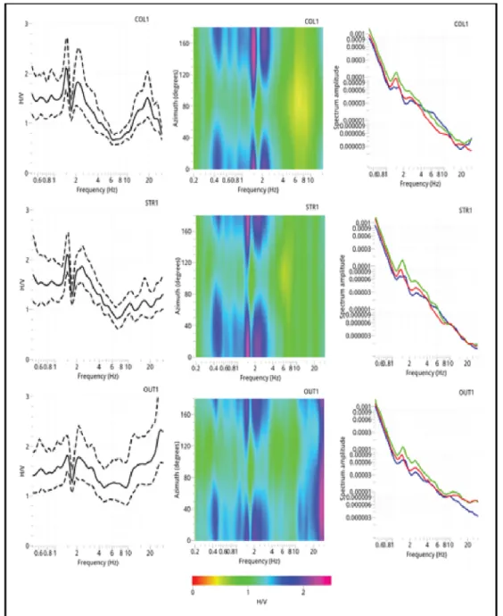
Figure 9 shows the H/V ratios obtained at each station, for clarity of thefigure we show the H/V mean curve and standard deviations computed for each measurement site. Figure 9 also reports the results of directional noise analysis and the mean FAS computed for the three different components (Z in blue, NS in green and EW in red) for each station. The H/V curves show a good agreement in terms of shape within the three sta-tions. Two peaks are observed at frequency of about 1.5 and 2.4 Hz in all sites. In all the three cases, the observed H/V peaks are due to signal characterized by energy higher on the horizontal's components com-pared to the vertical one, as clearly indicated by the FAS (Figure 9). Moreover, a clear polarization in the north and south directions is observed for the H/V peaks around the picks. Finally, also the amplitudes of

Figure 9. H/V spectral ratios for the three different sites in Cola Cave. The panels on the right show the average values of the spectral ratios with the relative standard deviations. Thefigure in the middle panels show the results of H/V rotated in the horizontal plane, i.e., as a function of azimuth. In the right side, the averaged Fourier Amplitude Spectra (FAS) for the three components of motion (blue curve refers to the vertical component). Each panel shows the code associated to the corresponding seismic stations (top right).

H/V peaks (mean values) are comparable within the three stations with values close to 2 or slightly less than 2 for the peaks at 1.5 Hz and of about 1.7 ÷ 1.8 for the higher frequency peaks. A further spectral peak around 15–20 Hz is present in only one measurement (COL1). Also, in this latter case, this peak is characterized by an amplitude value (of about 1.5) significantly lower than the threshold used to identify local seismic amplification effects from HV spectral ratios analysis.

Figure 10. Results of the simple modeling for thefive seismogenic sources. For each source, we computed the failure tensile strength (σ) along the speleothem axis for four different cases in order to explore the epistemic uncertainty in the modeling parameters (UHS and the densityρ). The dotted horizontal lines are the maximum and minimum threshold value of the failure tensile strength, beyond which the speleothem could collapse.

Figure 11. Results of the complex modeling for the two seismogenic sources that showed higher results in the simple modeling (Figure 10). Different from the simple modeling, here, the modeled failure tensile strength (σ) reaches the highest value at 0.2 meters, the same point where the speleothem is collapsed (Figure 5).

Summing up, the H/V curves at the sites show similar characteristics both in terms of fundamental frequen-cies and spectral shapes, the weak peaks observed (with amplitudes≤ 2) suggest no important amplification phenomena (SESAME criteria and guidelines, Bard & SEAME‐Team, 2005). Based on these results, we have not used the site contribution in theoretical spectral response simulated at the cave bedrock.

5.3. Numerical Modeling

The numerical modeling results, obtained with both the“simple” and “complex” models, show how the value of the tensile stress (σT) arising from seismic motion varies along the speleothem axis (Figures 10

and 11). In the“simple” modeling (Figure 10), the maximum values of σTare at the base of the speleothem,

and as we move upward the values decrease until they are null at the top. For three out of thefive seismo-genic sources for which seismic input was calculated, the minimum threshold value of tensile strength was not reached. This therefore means that a possible earthquake generated by seismogenic sources“Salto Valley,” “Campo Felice‐Ovindoli,” and “Velino” is not able to cause the collapse of the speleothem when a“simple” geometry is adopted. The “simple” modeling allowed us to make a skimming between the possi-ble sources that caused collapse of COLA‐3 and, based on results, we discarded the latter three sources in “complex” modeling.

In Figure 11, we compare the variations of the tensile stress valuesσTalong the speleothem axis with the

threshold values of tensile strength for the“complex” modeling using the input UHS obtained for the “Fucino” and “Liri” seismogenic sources. In this scenario, the maximum value of σTis not at the base of

the speleothem, but it increases from the base to a maximum point beyond which it decreases until zero at the top. This result is in excellent agreement with the geometric data of the modeled speleothem. Indeed, the maximum tensions that led to the speleothem breakage occurred at the exact point where the speleothem has a narrowing of its axis, which therefore represents a vulnerable section. This maximum value ofσTwas produced at ~22 cm height, which perfectly matches the elevation of the stump left by the

breakage (Figure 5). Results of the complex modeling show that only the seismogenic source“Liri” reaches the minimum threshold value of tensile strength, suggesting it is the most likely source of the earthquake recorded by the collapse of speleothem COLA‐3.

6. Discussion

Taken together, ages from pre‐event and postevent layers define three distinct speleoseismic events: the pre-penultimate with an age >12.5 ka, the pre-penultimate between ~7–14 and ~4–5 ka, and the ultimate after 1.1 ka (Table 5). We relate these events to paleoearthquakes that caused significant ground motion and collapses of cave speleothems. Unfortunately, pre‐event and postevent layers are only available for two speleothem cou-plets (COLA‐3/COLA‐1&2 and TRAP‐1/TRAP‐2) and refer to the penultimate event (or for the ultimate event for the latter couple). For the remaining events, either pre‐event or postevent ages are only defined (Table 5). In addition, a large time span separates pre‐event and postevent layers for the two speleothem cou-plets, impacting a tight definition of the age of the penultimate and possibly the ultimate events.

We can mitigate the above uncertainties and better refine the paleoearthquake age estimate based on the acceptable assumption that growth of postevent stalagmites occurred soon after the collapse of the spe-leothem upon which they grew. We do not consider in this approach sampling and measurement errors that are too small to match the large time gap observed.

For the penultimate event, although a significant time span is observed between pre‐event and postevent layers, the simplest interpretation is that the circulation‐precipitation system closed long before the event and was reopened by seismic shaking. We refer to this assumption as the postevent growth hypothesis. We are aware that closure and opening of the system could arise from changes in climatic and hydrologic conditions as well. However, we do not expect significant variations in the limited time span studied here when the Holocene climatic optimum was attained (Giraudi et al., 2011; Rossignol‐Strick, 1999). The hypothesis is corroborated by the observation that, when more than one single age determination is avail-able for postevent layers as in the case of COLA‐1, COLA‐2, and COLA‐4 from Room D, their value overlap or is very close. These ages may indicate a sudden opening of the circulation‐precipitation system in the limestone above Room D that in our view is related to seismic shaking during the penultimate event. The inverse hypothesis, that shaking closed the system that was fortuitously opened long after, seems untenable.

Bearing the above in mind, we suggest that the prepenultimate event occurred at or slightly before ~12.5 ka and is documented by a stalagmite (sample CRLL) grown on a large limestone block fallen from the vault of the cave in Room E (Figure 2). We compare this result with the paleoseismological data (trenches and 36Cl cosmogenic data; Galadini & Galli, 1999; Galli et al., 2008, 2012; Schlagenhauf et al., 2010, 2011; Palumbo et al., 2004) available for the“Fucino” source (Figure 8). Cosmogenic data iden-tified a possible exhumation event older than 14.7 ± 1 ka (Schlagenhauf et al., 2011) that could be the same identified in this work. An alternative view, that we regard as more likely based on the postevent growth hypothesis outlined above, is that the prepenultimate event relates to a faulting event found around 12.5 ka in paleoseismic trenches on the“Fucino” fault system (Galadini & Galli, 1999), which produced a signifi-cant vertical displacement (~3 m on SBGM fault and 1 and 2 m on the Trasacco fault, a secondary splay of the system).

Within the postgrowth hypothesis, the maximum age of the penultimate event is suggested by the oldest (COLA‐1) postevent layer at 5.1 ka, which, within uncertainty, could be as young as 4.8 ka (Table 5). Postevent layers COLA‐2 (on the same stalagmite) and COLA‐4 (on a nearby speleothem), with maximum ages of 4.3 and 3.8 ka, respectively, probably started growing some hundred to a thousand years after the fall. Comparison of our results for the penultimate event with the“Fucino” paleoseismological observations available from literature (Figure 8) does notfit perfectly the exhumation event recorded by Schlagenhauf et al. (2011) at 4.8 +0.3/−0.4 ka using 36Cl data on the Magnola fault plane or the trench record by Galadini and Galli (1999), where the closest event occurred between ~6.0 and 5.6 ka.

Finally, the pre‐event and postevent layers TRAP‐2 and TRAP‐1 brackets the ultimate event at ~8.0–1.5 ka, and COLA‐21 after 1.1 ka. Although the fall of TRAP‐2 could have occurred during the penultimate event, by considering the postgrowth hypothesis, we regard this fall as constrained by the 1.55 ± 0.07 ka age of TRAP‐ 1. In support of this, nearby stalactite COLA‐21 (Figure 2) fell on the ground after 0.91–1.34 ka. Considering uncertainties (Table 5), the two estimates may be separated by only 140 years; therefore, they are both assigned to the ultimate event.

The ultimate event can be compared to the trench rupture found between 426 and 782 CE on the Fucino fault (Figure 8; Galli et al., 2008). These authors attributed the trench offset to the earthquakes that hit Rome in 508 CE causing serious damages to the Coliseum (Galadini & Galli, 2001). The last36Cl exhumation found on the Magnola fault plane (Schlagenhauf et al., 2010, 2011) has an age comparable to the ultimate speleoseismic event as well. The Magnola fault represents the northern segment, closest to the Cola Cave, of the“Fucino” fault system. However, the damages occurred in the distant site of Rome suggest that the entire ~38 km fault system ruptured contemporarily (Galli et al., 2012). In principle, we cannot fully exclude that the ultimate speleoseismic event recorded in the cave occurred during the devastating 1915 Mw7

earth-quake, the strongest recorded in central Italy (Rovida et al., 2016). This earthquake was generated similarly by the entire“Fucino” fault system, with surface faulting recognized on several segments (Oddone, 1915) and an inferred rupture directivity from the SE towards the NW (Berardi et al., 1999).

For the penultimate event, we carried out a vulnerability analysis of COLA‐3 to find a direct attribution to a seismogenic source potentially responsible for the collapse. Using seismogenic source and seismic hazard models, we calculated the expected ground motion (i.e., Uniform Hazard Spectra) in the cave by the selected sources in turn, in a determinist approach, and compared it to the calculated failure tensile stress (σT) of the

stalagmite. The results suggest two possible seismogenic sources responsible of the collapse: the“Fucino” and the“Liri” sources. The “complex” modeling, where the speleothem diameter size varies along the axis, suggests“Liri” as the most likely source of the recorded shaking (see section 5.3). It is important to highlight that we explored uncertainties related to the variability in density and tensile strength, and the maximum expected magnitude and ground motion (i.e., Ground Motion Prediction Equations), but several other sources of error remain unquantified. The results could be affected, for example, by the rupture directivity, as happened for the 1915 earthquake, or by the actual hypocentre location, hypothesized in our modeling at the bottom of the fault rupture and in the center of the fault system. Besides, we cannot exclude that changes in orientation of C axes of calcite crystals in the speleothem, from horizontal at the base to vertical above, can create sections potentially prone to breakage even in case of weaker ground motions. Finally, we cannot exclude the general variations of the mechanical parameters, like for the example the densityδ, inside the stalagmite, that we considered homogeneous.

For these reasons, although the“Liri” fault remains the most likely source of the large paleoearthquakes recorded in the cave, and specifically of the penultimate event, we cannot exclude “Fucino” as another potential source. This alternative scenario may be supported by the possible directivity of the rupture towards NNW and a hypocentre closer to the Cola Cave during the speleoseismic events studied here. The “Liri” fault recent activity is debated, and no paleoseismological data on the fault are available to be com-pared to our event age. On the other hand, the abundance of paleoseismological data on the“Fucino” source renders the comparison possible, and we were able to match our speleoseismological data of two events (the ultimate and the prepenultimate) with the paleoseismological record.

7. Conclusions

Our study allowed to reconstruct the speleoseismological history of the Cola Cave in central Italy and to identify seismogenic sources potentially responsible for the collapse of a tall stalagmite and for two addi-tional speleoseismic events.

Using the samples ages and the comparison with available paleoseismological data for active faults in the region surrounding the cave, we identified three speleoseismic events: the prepenultimate occurred before but probably near ~12.5 ka, the penultimate occurred around ~5 ka, and the ultimate around ~1.5 ka and consistent with the 508 AD earthquake, which caused damages to the Coliseum in Rome.

The seismic hazard and vulnerability analysis of the tall stalagmite, collapsed during the penultimate event, allowed tofind a direct attribution to a seismogenic source potentially responsible for the collapse. Modeling suggests the“Liri” fault as the most likely seismogenic source responsible for the ground shaking. The“Fucino” fault system cannot be excluded as a potential source of collapsing in the cave. In support of this, the ages of two speleoseismic event matches some of the events found in trenches and on exhumed fault planes along the system.

We believe that the approach presented here can be useful to improve the paleoseismological data record available in active areas similar to the central Apennines, mainly collected using“classical” trench methods (e.g., Galli et al., 2008) or through more“innovative” investigations like fault surface exposure dating by cos-mogenic technique (e.g., Benedetti & Van Der Woerd, 2014; Tesson et al., 2016).

The numerical FEM approach, using the best approximation of the complex speleothem geometry, allows to evaluate in detail the speleothem behavior during ground motion, and to precisely define the point of break-age as the weakest section of the speleothem.

The integrated use of seismic hazard and speleothem vulnerability analysis allowed tofind a direct attribu-tion of the penultimate speleoseismological event to a seismogenic source and suggested as possible the activity of the“Liri” fault that should be considered more carefully into seismic hazard and risk models. Further developments of the approach could integrate fault segmentation relaxation and the possible fault interactions into the seismic hazard model (e.g., Valentini et al., 2020; Verdecchia et al., 2018; Visini et al., 2020) and a better treatment of the uncertainties involved in the definition of the mechanical proper-ties of broken speleothems and in the age record of speleoseismic events.

Data Availability Statement

All the parametric data for sample dating, seismogenic sources and the speleothems physical and mechan-ical data are reported in tables (Tables 1–4) and have been taken from published literature, listed in the refer-ences. Data supporting the sample dating can be found also in the Pangaea repository at https://doi.pangaea. de/10.1594/PANGAEA.922154 and https://doi.pangaea.de/10.1594/PANGAEA.922156.

References

Bard, P.‐Y., & SESAME‐Team (2005). Report D23.12, Guidelines for the Implementation of the H/V Spectral Ratio Technique on Ambient Vibrations Measurements, Processing and Interpretation in European Commission: Research General Directorate, Project No. EVG1‐CT‐ 2000‐00026 (p. 62). France: SESAME. available online at: https://sesame.geopsy.org/Papers/HV_User_Guidelines.pdf

Bar‐Matthews, M., Ayalon, A., Kaufman, A., & Wasserburg, G. J. (1999). The eastern Mediterranean paleoclimate as a reflection of regional events: Soreq cave, Israel. Earth and Planetary Science Letters, 166(1–2), 85–95. https://doi.org/10.1016/S0012-821X(98)00275-1 Becker, A., Davenport, C. A., Eichenberger, U., Gilli, E., Jeannin, P. Y., & Lacave, C. (2006). Speleoseismology: A critical perspective.

Journal of Seismology, 10(3), 371–388. https://doi.org/10.1007/s10950-006-9017-z

Acknowledgments

We sincerely thank S. Di Bianco, J. De Massis and P. Teodoro who helped sampling and collecting the cave data; F. Visini who helped us during the seismic noise measurements acquisition and discussed with us the seismic hazard results; D. Berardi who led us in the Cola Cave; F. Rizzo who helped us during the initial part of FEM modeling; S. Agostini for useful discussions on speleoseismology and for providing his papers collection. Finally, we would like to thank the Editor T. Schildgen, the Associate Editor L. Dal Zilio and the two reviewers C.P. Rajendran and J. Szczygieł for helpful comments and revisions that significantly improved the manuscript.

Becker, A., Häuselmann, P., Eikenberg, J., & Gilli, E. (2012). Active tectonics and earthquake destructions in caves of northern and Central Switzerland. International Journal of Speleology, 41(1), 35–49. https://doi.org/10.5038/1827-806X.41.1.5

Benedetti, L. C., & Van Der Woerd, J. (2014). Cosmogenic nuclide dating of earthquakes, faults, and toppled blocks. Elements, 10(5), 357–361. https://doi.org/10.2113/gselements.10.5.357

Berardi, R., Contri, P., Galli, P., Mendez, A., & Pacor, F. (1999). Modellazione degli effetti di amplificazione locale nelle città di Avezzano, Ortucchio e Sora. In S. Castenetto, & F. Galadini (Eds.), 13 gennaio del 1915 (pp. 349–372). Servizio Sismico Nazionale: Il terremoto nella Marsica.

Bindi, D., Pacor, F., Luzi, L., Puglia, R., Massa, M., Ameri, G., & Paolucci, R. (2011). Ground motion prediction equations derived from the Italian strong motion database. Bulletin of Earthquake Engineering, 9(6), 1899–1920. https://doi.org/10.1007/s10518-011-9313-z Boncio, P., Lavecchia, G., & Pace, B. (2004). Defining a model of 3D seismogenic sources for seismic hazard assessment applications: The

case of central Apennines (Italy). Journal of Seismology, 8(3), 407–425. https://doi.org/10.1023/B:JOSE.0000038449.78801.05 Bonnefoy‐Claudet, S., Cornou, C., Bard, P. Y., Cotton, F., Moczo, P., Kristek, J., & Fäh, D. (2006). H/V ratio: A tool for site effects

eva-luation. Results from 1‐D noise simulations. Geophysical Journal International, 167(2), 827–837. https://doi.org/10.1111/j.1365-246X.2006.03154.x

Bosi, C. (1975). Osservazioni preliminari su faglie probabilmente attive nell'Appennino centrale. Bollettino della Societa Geologica Italiana, 94(1975), 827–859.

Cadorin, J. F., Jongmans, D., Plumier, A., Camelbeeck, T., Delaby, S., & Quinif, Y. (2001). Modelling of speleothems failure in the Hotton cave (Belgium). Is the failure earthquake induced? Geologie En Mijnbouw/Netherlands Journal of Geosciences, 80(3–4), 315–321. https:// doi.org/10.1017/s001677460002391x

Cauzzi, C., Faccioli, E., Vanini, M., & Bianchini, A. (2015). Updated predictive equations for broadband (0.01–10 s) horizontal response spectra and peak ground motions, based on a global dataset of digital acceleration records. Bulletin of Earthquake Engineering, 13(6), 1587–1612. https://doi.org/10.1007/s10518-014-9685-y

Cheloni, D., De Novellis, V., Albano, M., Antonioli, A., Anzidei, M., Atzori, S., et al. (2017). Geodetic model of the 2016 Central Italy earthquake sequence inferred from InSAR and GPS data. Geophysical Research Letters, 44, 6778–6787. https://doi.org/10.1002/ 2017GL073580

Chiaraluce, L., Valoroso, L., Piccinini, D., Di Stefano, R., & De Gori, P. (2011). The anatomy of the 2009 L'Aquila normal fault system (Central Italy) imaged by high resolution foreshock and aftershock locations. Journal of Geophysical Research, 116, B12311. https://doi. org/10.1029/2011JB008352

Cinti, F. R., Pantosti, D., De Martini, P. M., Pucci, S., Civico, R., Pierdominici, S., et al. (2011). Evidence for surface faulting events along the Paganica fault prior to the 6 April 2009 L'Aquila earthquake (Central Italy). Journal of Geophysical Research, 116, B07308. https://doi. org/10.1029/2010JB007988

Colella, A., Cremona, M., Di Bianco, S., Ferranti, L., Ramondini, M., & Calcaterra, D. (2017). Valutazione dei principali parametrifisico‐ meccanici di alcuni speleotemi Italiani. In Atti III Convegno Regionale di Speleologia «Campania Speleologica», 2–4 Giugno 2017, Napoli, Italy(pp. 101–112). Bologna, Italy: Società Speleologica Italiana. ISBN: 978‐88‐89897‐16‐4

Columbu, A., De Waele, J., Forti, P., Montagna, P., Picotti, V., Pons‐Branchu, E., et al. (2015). Gypsum caves as indicators of climate‐driven incision and aggradation in a rapidly uplifting region. Geology, 43(6), 539–542. https://doi.org/10.1130/G36595.1

D'Agostino, N. (2014). Complete seismic release of tectonic strain and earthquake recurrence in the Apennines (Italy). Geophysical Research Letters, 41, 1155–1162. https://doi.org/10.1002/2014GL059230

Devoti, R., Esposito, A., Pietrantonio, G., Pisani, A. R., & Riguzzi, F. (2011). Evidence of large scale deformation patterns from GPS data in the Italian subduction boundary. Earth and Planetary Science Letters, 311(3–4), 230–241. https://doi.org/10.1016/j.epsl.2011.09.034 Di Domenica, A., & Pizzi, A. (2017). Defining a mid‐Holocene earthquake through speleoseismological and independent data: Implications

for the outer Central Apennines (Italy) seismotectonic framework. Solid Earth, 8(1), 161–176. https://doi.org/10.5194/se-8-161-2017 DISS Working Group (2015). Database of individual seismogenic sources (DISS), version 3.2.0: A compilation of potential sources for

earth-quakes larger than M 5.5 in Italy and surrounding areas. Rome, Italy: Istituto Nazionale di Geofisica e Vulcanologia. http://diss.rm.ingv. it/diss; https://doi.org/10.6092/INGV.IT‐DISS3.2.0

Faure Walker, J. (2014). Mechanics of continental extension from Quaternary strainfields in the Italian Apennines (PhD thesis). (p. 405). London, UK: University College London.

Ferranti, L., Pace, B., Valentini, A., Montagna, P., Pons‐Branchu, E., Tisnérat‐Laborde, N., & Maschio, L. (2019). Speleoseismological constraints on ground shaking threshold and seismogenic sources in the Pollino range (Calabria, southern Italy). Journal of Geophysical Research: Solid Earth, 124, 5192–5216. https://doi.org/10.1029/2018JB017000

Forti, P. (2001). Seismotectonic and paleoseismic studies from speleothems: The state of the art. Geologica Belgica, 4(3–4), 175–185. Retrieved from https://popups.uliege.be:443/1374‐8505/index.php?id=1981

Forti, P., Petrini, V., & Postpischl, D. (1981). Ricostruzione di fenomeni paleosismici da strutture carsiche. Rendiconti. Società Geologica Italiana, 1981(4), 563–569.

Forti, P., & Postpischl, D. (1980). Neotectonic data from stalagmites: Sampling and analysis techniques. In European Regional Conference on Speleology Sofia (Vol. 351, pp. 34–39). Sofia: CNR – Progetto Finalizzato Geodinamica.

Forti, P., & Postpischl, D. (1984). Seismotectonic and paleoseismic analyses using karst sediments. Marine Geology, 55(1–2), 145–161. https://doi.org/10.1016/0025-3227(84)90138-5

Galadini, F., & Galli, P. (1999). The Holocene paleoearthquakes on the 1915 Avezzano earthquake faults (Central Italy): Implications for active tectonics in the central Apennines. Tectonophysics, 308(1–2), 143–170. https://doi.org/10.1016/S0040-1951(99)00091-8 Galadini, F., & Galli, P. (2000). Active tectonics in the central Apennines (Italy)–input data for seismic hazard assessment. Natural

Hazards, 22(3), 225–268. https://doi.org/10.1023/A:1008149531980

Galadini, F., & Galli, P. (2001). Archaeoseismology in Italy: Case studies and implications on long‐term seismicity. Journal of Earthquake Engineering, 5(1), 35–68. https://doi.org/10.1142/S1363246901000236

Galadini, F., Galli, P., & Giraudi, C. (1997). Geological investigations of Italian earthquakes: New paleoseismological data from the Fucino Plain (Central Italy). Journal of Geodynamics, 24(1–4), 87–103. https://doi.org/10.1016/s0264-3707(96)00034-8

Galadini, F., & Messina, P. (2001). Plio‐quaternary changes of the normal fault architecture in the central Apennines (Italy). Geodinamica Acta, 14(6), 321–344. https://doi.org/10.1080/09853111.2001.10510727

Galadini, F., & Messina, P. (2004). Early‐middle Pleistocene eastward migration of the Abruzzi Apennine (Central Italy) extensional domain. Journal of Geodynamics, 37(1), 57–81. https://doi.org/10.1016/j.jog.2003.10.002

Galli, P., Galadini, F., & Pantosti, D. (2008). Twenty years of paleoseismology in Italy. Earth‐Science Reviews, 88(1–2), 89–117. https://doi. org/10.1016/j.earscirev.2008.01.001