HAL Id: hal-00703569
https://hal.archives-ouvertes.fr/hal-00703569
Submitted on 12 Jun 2012
HAL is a multi-disciplinary open access
archive for the deposit and dissemination of
sci-entific research documents, whether they are
pub-lished or not. The documents may come from
teaching and research institutions in France or
abroad, or from public or private research centers.
L’archive ouverte pluridisciplinaire HAL, est
destinée au dépôt et à la diffusion de documents
scientifiques de niveau recherche, publiés ou non,
émanant des établissements d’enseignement et de
recherche français ou étrangers, des laboratoires
publics ou privés.
Orientation of non-spherical particles in an
axisymmetric random flow
Dario Vincenzi
To cite this version:
Dario Vincenzi. Orientation of non-spherical particles in an axisymmetric random flow. Journal of
Fluid Mechanics, Cambridge University Press (CUP), 2013, 719, pp.465-487. �10.1017/jfm.2013.8�.
�hal-00703569�
Orientation of non-spherical particles in an
axisymmetric random flow
D A R I O V I N C E N Z I
CNRS UMR 7351, Laboratoire J.-A. Dieudonn´e, Universit´e de Nice Sophia Antipolis, Parc Valrose, 06108 Nice, France
The dynamics of non-spherical rigid particles immersed in an axisymmetric random flow is studied analytically. The motion of the particles is described by Jeffery’s equation; the random flow is Gaussian and has short correlation time. The stationary probability den-sity function of orientations is calculated exactly. Four regimes are identified depending on the statistical anisotropy of the flow and on the geometrical shape of the particle. If λ is the axis of symmetry of the flow, the four regimes are: rotation about λ, tum-bling motion between λ and−λ, combination of rotation and tumbling, and preferential alignment with a direction oblique to λ.
1. Introduction
Non-spherical solid particles suspended in a moving fluid rotate and orient themselves under the action of the velocity gradient. Even at low concentrations, the orientational dy-namics of non-spherical particles can influence the rheological properties of a suspension, namely the intrinsic viscosity and the normal stress coefficients (Bird et al. 1977; Larson 1999). This phenomenon has diverse practical applications. In the turbulent regime, for instance, the injection of rodlike polymers in a Newtonian fluid can produce a consider-able reduction of the turbulent drag, with this effect being routinely exploited to reduce energy losses in pipelines (Gyr & Bewersdorff 1995). The study of the orientation of parti-cles immersed in a fluid also has numerous applications in the natural sciences. Amongst them it is worth mentioning the swimming motion of certain biological micro-organisms (Saintillan & Shelley 2008; Koch & Subramanian 2011) and the formation of ice crystals in clouds (Chen & Lamb 1994). This latter phenomenon plays a crucial role in processes such as rain initiation and radiative transfer.
The starting point for understanding the properties of a dilute suspension is the motion of an isolated particle in a given flow field. Analytical results on the dynamics of a non-spherical particle have been obtained for various laminar flows, both steady and unsteady. Jeffery (1922) derived the equations of motion for an inertialess ellipsoid in a steady uniform shear flow at low Reynolds number. For a spheroid (i.e. an ellipsoid of revolution), Jeffery showed that the axis of symmetry of the particle performs a periodic motion on a closed orbit. Bretherton (1962) subsequently extended Jeffery’s analysis to particles of a more general shape: he demonstrated that, except for certain very long particles, the dynamics of any body of revolution transported by a low-Reynolds-number shear is equivalent to that of a spheroid with an effective aspect ratio. Amongst bodies of revolution, rigid dumbbells and rods have received a systematic investigation (Bird, Warner & Evans 1971; Doi & Edwards 1986).
In Jeffery’s (1922) and Bretherton’s (1962) derivations, not only fluid and particle inertia are disregarded, but also Brownian fluctuations due to the collisions of the particle with the molecules of the fluid. Nevertheless, if a particle is sufficiently small, molecular diffusion does influence its orientational dynamics, as was shown by Leal & Hinch (1971)
and Hinch & Leal (1972). The review article by Brenner (1974) collects analytical results on the motion of rigid neutrally buoyant bodies of revolution subject to a uniform velocity gradient and to Brownian fluctuations. A more recent review on this problem can be found in Petrie (1999). Finally, even in simple laminar flows, the orientation of particles can form complex patterns; this behaviour was studied by Szeri (1993) in the context of the theory of dynamical systems.
In turbulent flows and in some chaotic flows, the velocity gradient exhibits small-scale fluctuations. Thus, depending on the size of the particles, Jeffery’s assumption of a spa-tially uniform velocity gradient may not be applicable. To measure the probability of orientations, experiments have generally used relatively large particles, and therefore the velocity gradient could vary appreciably over the size of a particle (e.g. Krushkal & Gallily 1988; Bernstein & Shapiro 1994; Newsom & Bruce 1998; Parsheh, Brown & Aidun 2005; Parsa et al. 2011; Zimmermann et al. 2011a,b). Accordingly, theoretical studies were mainly concerned with the derivation of model equations for the probability of orien-tations, in which turbulent fluctuations were treated as an effective isotropic diffusion term (Olson & Kerekes 1998; Shin & Koch 2005). Jeffery’s approach, however, remains applicable to chaotic or turbulent flows provided that the particles are sufficiently small. The orientation dynamics of tiny elongated particles was studied numerically in chan-nel flows (Zhang et al. 2001; Mortensen et al. 2008a,b), in isotropic turbulence (Shin & Koch 2005; Pumir & Wilkinson 2011; Parsa et al. 2012), and in chaotic velocity fields (Wilkinson, Bezuglyy & Mehlig 2009). In contrast with the case of laminar flows, few analytical results seem to exist for the probability distribution of orientations of small particles transported by a turbulent or chaotic flow. Turitsyn (2007) examined the tum-bling motion of rodlike polymers in a random flow resulting from the superposition of a mean shear and of white-in-time isotropic fluctuations. Wilkinson & Kennard (2012) recently studied the alignment of rods with vorticity in a turbulent isotropic flow.
Here, the probability density function (p.d.f.) of orientations is derived exactly for small particles transported by a random flow with axisymmetric statistics. The particles are general bodies of revolution possessing fore-aft symmetry. The axisymmetry of the flow means that the velocity field is statistically invariant under arbitrary rotations of the axes about a given direction as well as under reflections in planes containing that direction or normal to it (Batchelor 1946; Chandrasekhar 1950). Axisymmetry is the simplest form of statistical anisotropy (Biferale & Procaccia 2005; Chang, Bewley & Bodenschatz 2012), and is found in rotating, stratified, or wind-tunnel turbulence (Lindborg 1995). Furthermore, the random flow is assumed to be Gaussian and to have zero correlation time. The assumption of temporal decorrelation is adequate when the correlation time of the flow is short compared to the characteristic time scale of material-line-element stretching. This assumption, albeit restrictive, allows a fully analytical solution of the problem.
The evolution equation for the orientation vector of a non-spherical rigid particle is introduced in§ 2. Section 3 is devoted to the derivation of the Fokker–Planck equation for the p.d.f. of the orientation angle. Its stationary solution is studied in § 4. Some conclusions are drawn in§ 5.
2. Orientation dynamics
The particles considered here are rigid bodies of revolution possessing fore-aft symme-try (although in the literature such particles are commonly referred to as “axisymmetric”, this terminology will be avoided here not to generate confusion; the term “axisymme-try” will be reserved to the statistical invariance of the velocity field). The particles
are of uniform composition and are suspended in a Newtonian fluid of the same den-sity. Furthermore, the inertia of the particles as well as hydrodynamic particle-particle interactions are disregarded, and no externally imposed force or couple influences the dynamics. In particular, it is appropriate to disregard hydrodynamic interactions when the suspension is sufficiently dilute.
The undisturbed motion of the fluid is described by the velocity field v(x, t). The size of the particles is assumed to be small compared to the typical length over which the velocity gradient ∇v = (∂jvi)16i,j63 changes (∂j ≡ ∂/∂xj). For turbulent flows,
this assumption is satisfied if the particles are smaller than the Kolmogorov scale, where viscosity smooths out the velocity fluctuations; the Reynolds number of the flow at the scale of a particle is thus less than 1. Given their small size, the particles also experience Brownian collisions with the molecules of the fluid.
In a sufficiently dilute suspension, attention can be restricted to the dynamics of a single isolated particle. The configuration of a body of revolution is determined by the position of its centre of mass, rc(t), and by the orientation of its axis of revolution, which
is specified by a unit vector N (t) parallel to the axis itself. As the particles are subject to Brownian fluctuations, their dynamics is random even in a laminar flow. Consider first a deterministic velocity field or a given realisation of a random velocity field. On the above assumptions, the centre of mass moves according to the following equation (e.g. Doi & Edwards 1986):
˙rc(t) = v(rc(t), t) +
p
DTζ(t), (2.1)
whereDT > 0 is the translational diffusion coefficient and ζ(t) is three-dimensional white
noise, i.e. a Gaussian stochastic process with
hζ(t)i = 0 and hζi(t + τ )ζj(t)i = δijδ(τ ) (2.2)
for all t, τ > 0 and i, j = 1, 2, 3. The orientation vector satisfies the following stochastic differential equation (summation over repeated indexes is implied):
˙ Ni= κij(t)Nj− κpq(t) NpNq |N|2 Ni+ p DRΣij(N )◦ ξj(t), |N(0)| = 1, (2.3) where κ(t) = Ω(t) + γE (t) (2.4) with Ω(t) = G(t)− G T(t) 2 , E(t) = G(t) + GT(t) 2 , (2.5)
and G (t) = ∇v(rc(t), t). Thus, Ω(t) and E (t) are the vorticity tensor and the
rate-of-strain tensor evaluated at rc(t) and κ(t) is an effective Lagrangian velocity gradient.
The scalar constant γ depends on the geometrical shape of the particle. For |γ| < 1, the evolution equation can be mapped into that of a spheroid with aspect ratio equal to p(1 + γ)/(1− γ) (Bretherton 1962). Prolate spheroids are obtained for 0 < γ < 1, oblate spheroids for −1 < γ < 0. Special cases are: spheres (γ = 0), rigid dumbbells (γ = 1), rods (γ = 1), and disks (γ = −1). Furthermore, it was shown by Bretherton (1962) that in principle there exist very long particles for which |γ| > 1. In (2.3), the random vector ξ(t) is three-dimensional white noise and hence has the same properties as ζ(t), but is statistically independent of it. The matrix Σ (n) has the following form:
Σ(n) = I− nn/|n|2 (2.6) andDR> 0 is the rotary diffusion coefficient. By using the Cauchy–Schwarz inequality,
it is easy to check that Σ (n) is positive semi-definite. The symbol◦ indicates that the stochastic term in (2.3) is understood in the Stratonovich sense.
Equation (2.3) is Jeffery’s equation for the orientation vector of a body of revolution with the addition of a stochastic term modelling Brownian fluctuations. The stochastic term is chosen in such a way as to produce isotropic diffusion of N (t) on the unit sphere, so that|N(t)| is preserved in time (see appendix A for more details). It is worth remarking that a Brownian term of the same form has been used to model the turbulent fluctuations of the velocity gradient (Krushkal & Gallily 1988; Olson & Kerekes 1998; Shin & Koch 2005) or to describe particle–particle interactions both in semi-dilute suspensions (Doi & Edwards 1986) and in concentrated suspensions (Doi & Edwards 1978; Kuzuu & Doi 1980).
Equation (2.3) can be generalised to the case of a homogeneous axisymmetric random flow. The velocity field transporting the particle is Gaussian and has zero mean and correlation:
hvi(x + r, t + τ )vj(x, t)i = Qij(r)δ(τ ), i, j = 1, 2, 3. (2.7)
The form of the correlation guarantees that v(x, t) is statistically homogeneous in space. Additionally, the velocity field is assumed to be incompressible (∇ · v = 0) and statis-tically axisymmetric with respect to the direction specified by the unit vector λ. The tensor Q(r) must then take the form:
Qij(r) = Arirj+ Bδij+ Cλiλj+ D(riλj+ λirj), (2.8)
where A, B, C, D are smooth functions of|r|2and (r ·λ); A, B, and C are even in (r ·λ),
while D is odd in (r · λ) (Batchelor 1946; Chandrasekhar 1950). Furthermore, the func-tions A, B, C, D are not independent and satisfy certain differential relafunc-tions (Batchelor 1946; Chandrasekhar 1950). The velocity field defined above is an axisymmetric gener-alisation of the isotropic random flow introduced by Kraichnan (1968) in the context of passive turbulent transport. The same axisymmetric velocity field was used by Shaqfeh & Koch (1992) to study polymer stretching in flows through random beds of fibres.
The velocity gradient is also Gaussian and zero-mean; the single-point two-time cor-relation can be derived by using the statistical homogeneity of the velocity field:
h∂jvi(x, t + τ )∂qvp(x, t)i = Γijpqδ(τ ) i, j, p, q = 1, 2, 3 (2.9) with Γijpq=− ∂2Qip ∂rj∂rq ¯ ¯ ¯ ¯ r=0 . (2.10)
Substituting (2.8) in (2.10) yields (see equation (5.12) in Batchelor (1946)): Γijpq= (d + 4a)δjqδip− a(δpqδij+ δiqδpj) + (b + c + 5d)δjqλiλp− bδipλjλq
− d[(δpqλi+ δiqλp)λj+ (δpjλi+ δijλp)λq]− cλiλpλjλq,
(2.11) where a, b, c, d are real constants. For the sake of simplicity, λ is taken in the direction of the third axis, i.e. λ = (0, 0, 1). Then, the coefficients in Γijpq are written:
2a = Γ1212− Γ1111 d = Γ3333− Γ1111
b = Γ1212− Γ1313 2a + b + c + 4d = Γ3131− Γ3333.
(2.12)
The two-time correlation of the components of the vorticity ω = ∇× v can be expressed in terms of a, c, and d as follows (Batchelor 1946, p. 490):
and
hω3(x, t + τ )ω3(x, t)i = (10a + 2d)δ(τ). (2.14)
The coefficients a, b, c, d are not free; they are constrained by the following inequalities (see appendix B): ( a + d > 0 if a > 0, 5a + d > 0 if a < 0, (2.15a) 4a− b + d > 0, 4a + b + c + 6d > 0, (2.15b) 15a2− b2− (b − d)(c + 5d) + 2a(2c + 13d) > 0. (2.15c)
If a > 0 and b = c = d = 0, then Γijpq gives the single-point correlation of the gradient
of an isotropic velocity field (Robertson 1940). Thus, a determines the intensity of the isotropic part of the gradient and b, c, d control the statistical anisotropy of the flow.
The orientation dynamics of the particle depends on the velocity gradient evaluated at rc(t), which was denoted as G (t) in§ 2. In virtue of the δ-correlation in time and the
statistical homogeneity of the flow, G (t) has the same temporal statistics as ∇v(x, t) for any given x (Falkovich, Gaw¸edzki & Vergassola 2001) (the presence of white noise in (2.1) does not modify the statistics of G (t)). The components of κ(t), defined in (2.4), are a linear combination of the components of G (t), and consequently κ(t) is a Gaussian process with zero mean and correlation:
hκij(t + τ )κpq(t)i = Kijpqδ(τ ) (2.16)
with Kijpq=
1
4[Γijpq−Γijqp−Γjipq+Γjiqp+2γ(Γijpq−Γjiqp)+γ
2(Γ
ijpq+Γijqp+Γjipq+Γjiqp)].
(2.17) The form of Kijpq can be derived by substituting (2.4) and (2.5) into the left-hand
side of (2.16) and by using (2.9). The tensor Kijpq is positive semi-definite, for it is
the covariance of a second-order Gaussian tensor. Thus, in the evolution equation for the orientation vector, κ(t) plays the role of a multiplicative tensorial white noise. As κ(t) can be thought of as an approximation of a real noise process in the limit of zero correlation time, the corresponding terms in (2.3) must be interpreted in the Stratonovich sense (e.g. Kloeden & Platen 1992, p. 227). The stochastic differential equation for the orientation vector of a non-spherical particle can then be rewritten as follows:
˙
Ni= Mipq(N )◦ κpq(t) +
p
DRΣij(N )◦ ξj(t), (2.18)
where Mipq(n) = (δipδjk− δikδjp)njnknq/|n|2 and the initial condition N (0) is such
that|N(0)| = 1.
3. Fokker–Planck equation for the probability density function of the
orientation angle
As v(x, t) is statistically invariant under spatial translations, the p.d.f. of N (t) taking the value n = (n1, n2, n3) at time t is independent of rc and is thus denoted by f (n; t).
The Itˆo equation equivalent to (2.18) is ˙
Ni= βi(N ) + Mipq(N )κpq(t) +
p
Figure 1.Orientation of a non-spherical particle. with βi(n) = 1 2KmnpqMjpq(n) ∂ ∂njMimn(n) + DR 2 Σjk(n) ∂ ∂njΣik(n). (3.2) Consequently, f (n; t) satisfies the Fokker–Planck equation:
∂f ∂t =− ∂ ∂ni[βi(n)f ] + 1 2 ∂2 ∂ni∂nj [αij(n)f ] (3.3) with αij(n) = KmnpqMimn(n)Mjpq(n) +DRΣik(n)Σjk(n) = KmnpqMimn(n)Mjpq(n) +DRΣij(n), (3.4)
where the last equality follows from (A 3). Equations (3.1) and (3.3) can be derived from (2.18) by using the formal rules κij(t)dt = O(√dt) and κij(t)dt κpq(t)dt = Kijpqdt
and by proceeding as in the case of a vectorial white noise (see Gardiner 1983 and the appendix in Falkovich et al. 2001). The diffusion tensor α is positive semi-definite as a consequence of the positive semi-definiteness of K and Σ .
To study the orientation dynamics of a non-spherical particle, it is convenient to move from Cartesian coordinates (n1, n2, n3) to spherical coordinates (n, ϑ, ϕ) according to the
usual transformations: n =qn2 1+ n22+ n23, ϑ = arctan ³q n2 1+ n22/n3 ´ , ϕ = arctan(n2/n1) (3.5)
with 0 6 n, 0 6 ϑ 6 π, and 0 6 ϕ < 2π (figure 1). On account of the fixed length of the orientation vector, the probability density function of orientations must take the form f (n, ϑ, ϕ; t) = ψ(ϑ, ϕ; t)δ(n−L) with L = 1. Thus, ψ(ϑ, ϕ; t) sin ϑ dϑ dϕ is the probability of the particle being oriented at time t within an elementary solid angle sin ϑ dϑ dϕ of (ϑ, ϕ). In addition, the following normalisation holds:
Z π 0
Z 2π 0
ψ(ϑ, ϕ; t) sin ϑ dϑ dϕ = 1 ∀ t > 0. (3.6) The function Ψ (ϑ, ϕ; t) = ψ(ϑ, ϕ; t) sin ϑ satisfies a new Fokker–Planck equation, which can be derived from (3.3) by using the transformation formulae for the drift and diffusion coefficients under a change of variables (Risken 1989, p. 88), by writing f (n, ϑ, ϕ; t) = ψ(ϑ, ϕ; t)δ(n− L) with L = 1, and by integrating the resulting equation with respect
to n. The final result is: ∂Ψ ∂t =− ∂ ∂ϑ[Bϑ(ϑ)Ψ ] + 1 2 ∂2 ∂ϑ2[Aϑϑ(ϑ)Ψ ] + 1 2Aϕϕ(ϑ) ∂2Ψ ∂ϕ2, (3.7) where Bϑ(ϑ) = βi(n) ∂ϑ ∂ni +αij(n) 2 ∂2ϑ ∂ni∂nj =£µ1+ µ2sin2(ϑ) + µ3sin4(ϑ) ¤ cot ϑ,(3.8a) Aϑϑ(ϑ) = αij(n) ∂ϑ ∂ni ∂ϑ ∂nj = 2µ1+ µ4sin2(ϑ) + µ3sin4(ϑ), (3.8b) Aϕϕ(ϑ) = αij(n) ∂ϕ ∂ni ∂ϕ ∂nj = µ5+ 2µ1csc2(ϑ) (3.8c) with µ1=18£2(5 + 3γ2)a− 4γb + (1 − γ)2c + (9− 10γ + 5γ2)d + 4D′R ¤ , (3.9a) µ2=34γ [2b + (1− γ)c + (5 − γ)d] , (3.9b) µ3= cγ2, (3.9c) µ4= γ[2b + (1− γ)c + 5d], (3.9d) µ5=14 £ 4bγ− (1 − γ)2c − (1 − γ)(7 − 3γ)d¤, (3.9e) and D′
R =DR/L2 with L = 1 (the numerical values of D′R and DR coincide, but their
physical dimensions are different). Equations (3.8) involve the Jacobian and the Hessian of the transformation from Cartesian to spherical coordinates, which can be calculated from (3.5). Inequalities (2.15) guarantee that Aϑϑ(ϑ) and Aϕϕ(ϑ) are strictly positive
(appendix B).
The contribution to (3.7) due to the isotropic part of Γ is a Laplace–Beltrami term with diffusion coefficient proportional to a; this contribution is of the same form as that coming from ξ(t). The isotropic component of the flow and the Brownian fluctuations therefore have the same effect on the orientation statistics of the particle.
Since ϑ and ϕ are angular variables, the boundary conditions for Ψ (ϑ, ϕ; t) are periodic: Ψ (ϑ, ϕ; t) = Ψ (ϑ + 2π, ϕ; t) and Ψ (ϑ, ϕ; t) = Ψ (ϑ, ϕ + 2π; t) (3.10) for all ϑ, ϕ, and t. The long-time properties of Ψ (ϑ, ϕ; t) can be deduced from (3.7). If the partial derivative with respect to time is dropped, then (3.7) is invariant under the transformations ϑ↔ 2π − ϑ (reflections with respect to planes containing λ) and ϑ ↔ π− ϑ (reflections with respect to planes orthogonal to λ). Moreover, the coefficients Bϑ, Aϑϑ, andAϕϕdo not depend on ϕ (invariance under rotations about λ). These properties
of (3.7) are a natural consequence of the statistical axisymmetry of the velocity field and translate into analogous properties of the stationary p.d.f. of orientations.
The invariance of (3.7) under rotations about λ can be used to derive a one-dimensional Fokker–Planck equation for the marginal p.d.f.: bΨ (ϑ; t) = bψ(ϑ; t) sin ϑ with bψ(ϑ; t) = R2π
0 ψ(ϑ, ϕ; t)dϕ. Integrating (3.7) with respect to ϕ from 0 to 2π and making use of (3.10)
yield: ∂Ψb ∂t =− ∂ ∂ϑ h Bϑ(ϑ) bΨ i +1 2 ∂2 ∂ϑ2 h Aϑϑ(ϑ) bΨ i . (3.11)
The solution of the above equation must be normalised and periodic: bΨ (ϑ; t) = bΨ (ϑ+2π; t) for all ϑ, t. A direct consequence of (3.11) is that, along the trajectory of the particle, the time evolution of ϑ(t) is decoupled from that of ϕ(t) and is described by the stochastic
ordinary differential equation: ˙
ϑ(t) =Bϑ(ϑ(t)) +
p
Aϑϑ(ϑ(t)) η(t), 0 6 ϑ(t) 6 π, (3.12)
where η(t) is white noise.
4. Stationary statistics of the orientation angle
It was argued in§ 3 that the stationary solution of (3.7), Ψst, does not depend on ϕ.
Therefore, Ψst solves the equation:
1 2 d2 dϑ2[Aϑϑ(ϑ)Ψst]− d dϑ[Bϑ(ϑ)Ψst] = 0. (4.1) Thanks to the periodic boundary conditions (3.10), Ψst(ϑ) takes the following simple
form (see appendix C):
Ψst(ϑ) = N Aϑϑ(ϑ) exp " 2 Z ϑ ϑ0 Bϑ(z) Aϑϑ(z) dz # , (4.2)
where 0 6 ϑ06 πandN is a normalisation constant such that
2π Z π
0
Ψst(ϑ)dϑ = 1. (4.3)
In (4.2), the choice of ϑ0 is in fact unimportant, since it only modifies the normalisation
constant.
Only the case µ36= 0 is considered here; the case µ3 = 0 is examined in appendix D,
even though no new physical regimes emerge in this latter case. For µ36= 0, the integral
in (4.2) can be calculated by using the change of variable y = sin2(ω) and formulae 2.172, 2.175(1), and 2.177(1) of Gradshteyn & Ryzhik (1965). The final result is:
ψst(ϑ) = N χ(ϑ) [Aϑϑ(ϑ)]3/4 , (4.4) where χ(ϑ) = exp ½ 2 √ ∆ µ µ2− 3 4µ4 ¶ arctan · µ4+ 2µ3sin2(ϑ) √ ∆ ¸¾ (∆ > 0) exp ½µ3 4µ4− µ2 ¶ 2 µ4+ 2µ3sin2(ϑ) ¾ (∆ = 0) ¯ ¯ ¯ ¯ √ −∆ + µ4+ 2µ3sin2(ϑ) √ −∆ − µ4− 2µ3sin2(ϑ) ¯ ¯ ¯ ¯ 1 √ −∆( 3 4µ4−µ2) (∆ < 0) (4.5)
with ∆ = 8µ1µ3− µ24. It is shown in appendix B that ψst(ϑ) is bounded for all values
of a, b, c, d, and γ. The stationary p.d.f. of orientations satisfies ψst(2π− ϑ) = ψst(ϑ)
and ψst(π−ϑ) = ψst(ϑ). These properties are a consequence of the statistical symmetries
of the carrier flow, as was noted after (3.10).
Since ∆ can be written as ∆ = a2F (γ, b/a, c/a, d/a,D′
R/a), ψst(ϑ) only depends on
the ratios b/a, c/a, d/a,D′
R/a (and on γ). The same conclusion could have been reached
by rescaling t by a−1in (3.7).
For a spherical particle (i.e. γ = 0), µ2 and µ4 vanish. Consequently, χ(ϑ) = 1,
Aϑϑ(ϑ) = const., and hence ψst(ϑ) = (4π)−1, in accordance with the fact that all
orien-tations are equally probable for a sphere. Similarly, if a orD′
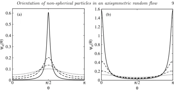
0 0.1 0.2 0.3 0.4 0.5 0.6 0 π/2 π ψst (θ) θ (a) 0 0.2 0.4 0.6 0.8 1 1.2 1.4 1.6 π π/2 0 ψst (θ) θ (b)
Figure 2.Stationary p.d.f. of the orientation angle ϑ. (a) Rotation about λ: b/a = 4.8, c/a = 55, d/a = 0.85, D′
R/a = 10−2, and γ = −1 (solid line), γ = −0.75 (dashed line), γ = −0.5
(dot-dashed line), γ = −0.25 (dotted line). (b) Tumbling motion between λ and −λ: b/a = 4.75, c/a = 10, d/a = 0.9, D′
R/a = 10−2, and γ = 1 (solid line), γ = 0.75 (dashed line), γ = 0.5
(dot-dashed line), γ = 0.25 (dotted line). The normalisation coefficient N has been computed numerically according to (4.3).
c, d, i.e. if the isotropic component of the velocity field or the Brownian fluctuations prevail on the anisotropic component of the flow, then µ1À µi, i = 2, . . . , 5 and ψst(ϑ)
weakly depends on ϑ regardless of the shape of the particle. In the following, therefore, γ is assumed to be nonzero and b, c, d are of the same order of magnitude as a andD′
R
or greater.
The behaviour of ψst(ϑ) can be deduced from that of its first derivative. By
us-ingAϑϑ(ϑ) > 0, it can be shown that, for all values of ∆,
d
dϑψst(ϑ) = γ sin(2ϑ)[cγ cos(2ϑ)− σ]h(ϑ), (4.6) where
σ≡ 2b + c + (5 + γ)d (4.7) and h(ϑ) is a strictly positive function for all 0 6 ϑ 6 π. Four regimes are then identified depending on the properties of the axisymmetric flow and on the geometrical shape of the particle:
(i) Rotation about the axis of symmetry of the flow. For the following values of the parameters:
|σ| > |cγ| and γσ < 0, (4.8) the function ψstonly has three extrema in ϑ = 0, π/2, π (indeed the equation cγ cos(2ϑ) =
σ has no solution). More precisely, ψst(ϑ) has a maximum in π/2 and two minima in 0
and π (figure 2). Thus, in this regime the particle rotates about the direction λ; the level of alignment with the plane perpendicular to λ decreases as the degree of anisotropy of the flow vanishes or the shape of the particle approaches the spherical one (figure 2).
(ii) Tumbling motion. In the following regime:
|σ| > |cγ| and γσ > 0, (4.9) ψst has three extrema: a minimum in π/2 and two maxima in 0 and in π (figure 2).
0 0.02 0.04 0.06 0.08 0.1 0.12 0.14 0.16 π π/2 0 ψst (θ) θ (a) 0 0.02 0.04 0.06 0.08 0.1 0.12 0.14 0.16 π π/2 0 ψst (θ) θ (b)
Figure 3.Stationary p.d.f. of the orientation angle ϑ. (a) Preferential alignment with a direction oblique to λ: γ = 1, D′
R/a = 10−2, b/a = −6, d/a = −0.9, and c/a = 55 (dashed line), c/a = 25
(solid line), c/a = 11 (dot-dashed line). (b) Combination of rotation and tumbling: γ = 1, D′
R/a = 10−2, c/a = −10, d/a = 1, and b/a = 1.1 (dot-dashed line), b/a = 2 (solid line),
b/a = 3 (dashed line). The p.d.f. has been normalised numerically according to (4.3).
The particle tumbles between the direction parallel to λ and that antiparallel to λ. The probability of the orientation angle ϑ being in the neighbourhood of 0 or π depends on the anisotropy degree of the flow and on the shape of the particle (figure 2).
(iii) Preferential alignment with a direction oblique to the axis of symmetry of the flow. If
|σ| < |cγ| and c > 0, (4.10) then ψst has three minima in 0, π/2, π and two maxima in ϑ⋆ and π− ϑ⋆, where 0 <
ϑ⋆< π/2 is such that sin ϑ⋆= s 1 2 µ 1−cγσ ¶ . (4.11)
The particle therefore spends most of the time at an angle ϑ⋆ (or π− ϑ⋆) with respect
to λ (figure 3).
(iv) Combination of rotation and tumbling. For
|σ| < |cγ| and c < 0, (4.12) the function ψst has three maxima in 0, π/2, π and two minima in ϑ⋆and π− ϑ⋆with ϑ⋆
defined in (4.11). In this regime, the particle preferentially lies either in the plane per-pendicular to λ, in the direction parallel to λ, or in the direction antiparallel to it.
Naturally, the coefficient a controlling the intensity of the isotropic component of the flow does not play any role in the above classification; the dynamical regime is selected by b, c, d, and by the shape coefficient γ. Whereas sufficiently elongated or flattened spheroids can be strongly aligned in regimes (i) and (ii), the ability of the flow to orient particles is weaker in regimes (iii) and (iv). In these regimes, stronger alignment can be obtained for|γ| > 1 (figure 4). Nevertheless, Bretherton (1962) observed that particles with |γ| > 1 may be unrealistic, albeit conceivable from a purely geometrical point of view.
0 0.05 0.1 0.15 0.2 π π/2 0 ψst (θ) θ (a) 0 0.05 0.1 0.15 0.2 π π/2 0 ψst (θ) θ (b)
Figure 4.Stationary p.d.f. of the orientation angle ϑ for |γ| > 1. (a) Preferential alignment with a direction oblique to λ: γ = 5, D′
R/a = 10−2, b/a = −6, c/a = 25, d/a = −0.9. (b)
Combination of rotation and tumbling: γ = 5, D′
R/a = 10−2, b/a = 2, c/a = −10, d/a = 1.
τ )∂3v3(x, t)i, i.e. if d = 0. In this case, µ2 = 3µ4/4 and hence ψst(ϑ) =N [Aϑϑ(ϑ)]−3/4;
furthermore, σ does not depend on γ. It then follows from (4.8) and (4.9) that if the particles with shape coefficient bγ rotate in the plane orthogonal to λ (resp. tumble), the particles with shape coefficient −bγ tumble (resp. rotate in the plane orthogonal to λ). By contrast, regimes (iii) and (iv) are independent on the sign of γ, i.e. on whether the particle is elongated or flattened, although ϑ⋆ changes when the sign of γ changes.
Moreover, if the particles with shape coefficient bγ rotate about λ (resp. tumbles), then all particles with|γ| < |bγ| and sgn(γ) = sgn(bγ) rotate about λ (resp. tumble). Similarly, if the particles with shape coefficient bγ are in regime (iii) (resp. in regime (iv)), then all particles with |γ| > |bγ| are in regime (iii) (resp. in regime (iv)). These properties, however, do not generally hold true if d is nonzero. For instance, if b/a =−4.4, c/a = 0.5, d/a = 1.5, then particles tumble for 1 > γ > 0.8, they have a preferential orientation for 0.8 > γ > 0.4, they rotate for 0.4 > γ > 0, and they tumble again for 0 > γ >−1.
5. Conclusions
Axisymmetric turbulence arises as one of the simplest frameworks in which to study the orientation dynamics of non-spherical particles. On the assumptions of Gaussianity and short correlation in time, it was shown analytically that the dynamics of a non-spherical particle immersed in a random axisymmetric flow exhibits four regimes: rotation around the axis of symmetry of the flow, tumbling, combination of rotation and tumbling, and preferential alignment with a direction oblique to the axis of symmetry of the flow. The regime is selected by the form of the anisotropic component of the flow and by the geometrical shape of the particle. If the flow is weakly anisotropic or if the particle is almost spherical, the mathematical description of ψst(ϑ) in terms of minima and maxima
remains formally valid, but the above physical classification loses its meaning, since ψst(ϑ)
does not differ appreciably from the uniform distribution.
The tumbling motion of a non-spherical particle in the axisymmetric random flow dif-fers from that of a rod immersed in the flow resulting from the superposition of a uniform shear and of a short-correlated isotropic random component (Puliafito & Turitsyn 2005; Turitsyn 2007). In the presence of a strong mean shear, the tumbling dynamics of a rod
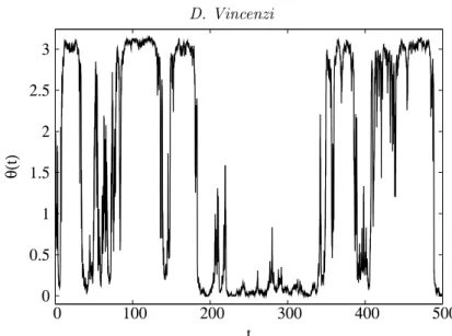
0 0.5 1 1.5 2 2.5 3 0 100 200 300 400 500 θ( t) t
Figure 5.A typical time evolution of ϑ(t) in the tumbling regime (γ = 1, b/a = 4.75, c/a = 10, d/a = 0.9, D′
R/a = 10−2); ϑ(t) has been computed by numerically integrating (3.12).
consists of aperiodic transitions between two unstable states: the one aligned with the direction of the shear and that anti-aligned with it. When a fluctuation takes the rod away from the aligned or anti-aligned state and moves it into the unstable region of the flow the mean shear makes the rod flip. By contrast, in the axisymmetric case, large deviations of the orientation of the particle from the axis of symmetry of the flow do not necessarily result into sudden flips of the particle (figure 5). Simply, the orientation vector of the particle fluctuates randomly, but the orientations aligned and anti-aligned with the axis of symmetry of the flow are much more probable than the other orienta-tions. Thus, there can be excursions of ϑ(t) from ϑ≈ 0 to ϑ ≈ π/2 followed by a return to ϑ ≈ 0 (figure 5). This behaviour would not be possible in the presence of a strong mean shear.
The axisymmetric random flow and the laminar uniform shear differ in the dependence of the orientation dynamics on the geometrical shape of particles. In a uniform shear flow, the motion of a rod or of a disc represents a degenerate case of the dynamics of non-spherical particles (Jeffery 1922). Moreover, the dynamics is qualitatively different for|γ| < 1 and |γ| > 1 (Bretherton 1962). In the axisymmetric random flow, the dynamics of particles changes smoothly as a function of the shape coefficient.
Finally, it is worth remarking that the function χ defined in (4.5) also determines the probability distribution of Jeffery’s orbits in the presence of weak Brownian fluctuations (Leal & Hinch 1971). There does not seem to be, however, a simple relation between the orientation dynamics in the uniform shear and that in the axisymmetric random flow.
The author is grateful to J´er´emie Bec, Antonio Celani, Fran¸cois Delarue, Prasad Per-lekar, Raymond Shaw, and Michael Wilkinson for useful suggestions. This work was supported in part by the French National Research Agency (ANR) under grant BLAN07-1 BLAN07-192604 “Dynamique et statistique des particules en turbulence” and by the EU COST Action MP0806 “Particles in turbulence”.
Appendix A. Rotary diffusion
Rotary diffusion is introduced in the dynamics of N (t) by assuming that its effect is to produce isotropic Brownian fluctuations of the direction of N (t), but not of its length. Mathematically, this is obtained by adding a Laplacian term to the equation for f (n; t) which acts only on the orientation of n. For a deterministic flow, f (n; t) thus satisfies (e.g. Leal & Hinch 1971; Hinch & Leal 1972; Brenner 1974; Bird et al. 1977; Doi & Edwards 1986): ∂tf =− e∇ ·[w(n, t)f ] + DR 2 ∇e 2f, (A 1) where e ∇≡ Σ (n) · ∇n (A 2) with Σ (n) = I− nn/|n|2 and ∇
n= (∂/∂n1, ∂/∂n2, ∂/∂n3). The differential operator e∇
is the angular part of the gradient or, equivalently, the restriction of the gradient to the sphere of radius|n|. In (A 1), e∇2
≡ e∇ ·∇e and w(n, t) = κ(t) · n− [κ(t) : nn]n/|n|2. The matrix Σ satisfies:
Σ = ΣT= Σ2, n× [∇n·Σ(n)] = 0, Σ(n) · n = 0. (A 3)
By using properties (A 3) and w(n, t) · n = 0, it is possible to rewrite (A 1) as follows: ∂f ∂t =− ∂ ∂ni[wi(n, t)f ] + DR 2 ∂ ∂niΣik(n) ∂ ∂njΣjk(n)f. (A 4) Equation (2.3) is the Stratonovich stochastic differential equation associated with (A 4). It is worth noting that given that the orientation vector has unit length, f (n; t) must take the form f (n; t) = F (n; t)δ(|n| − 1) with ∂F/∂n = 0. It would therefore be more natural to consider the evolution equation for F (n; t) instead of that for f (n; t); this is indeed the usual approach in the literature (Leal & Hinch 1971; Hinch & Leal 1972; Brenner 1974; Bird et al. 1977; Doi & Edwards 1986). In the present context, however, it is easier to formulate the problem in R3 and to move to angular variables afterwards.
Appendix B. Positive semi-definiteness of the covariance tensor
The fourth-order tensor Γ is the covariance of a Gaussian second-order tensor, and must therefore be positive semi-definite, i.e.
X
16i,j,p,q63
UijΓijpqUpq>0 (B 1)
for all second-order tensors U. Inequality (B 1) can be reinterpreted within the theory of positive semi-definite second-order tensors (e.g. Moakher 2008). Consider an invertible map ℓ which assigns to each pair of indices (i, j), 1 6 i, j 6 3, a single index ℓ(i, j) ranging from 1 to 9. By means of the map ℓ, U can be regarded as a 9-dimensional vector; likewise, Γ can be regarded as a symmetric 9× 9 second-order tensor, whose symmetry follows from Γijpq = Γpqij. Accordingly, (B 1) can be rewritten in the following form:
X
16ℓ(i,j),ℓ(p,q)69
Uℓ(i,j)Γℓ(i,j)ℓ(p,q)Uℓ(p,q)>0. (B 2)
Inequality (B 2) is the definition of positive semi-definiteness for second-order tensors. The theory of such tensors says that a necessary and sufficient condition for an Hermi-tian second-order tensor to be positive semi-definite is that all the principal minors of
the tensor are non-negative (Gantmacher 1959, p. 307). When this condition is applied to Γℓ(i,j)ℓ(p,q) it yields the following inequalities:
( a + d > 0 if a > 0 5a + d > 0 if a < 0 (B 3) and ̟1≡ 4a − b + d > 0, ̟2≡ 4a + b + c + 6d > 0, (B 4) ̟3≡ 15a2− b2− (b − d)(c + 5d) + 2a(2c + 13d) > 0. (B 5)
In this paper, the above inequalities are assumed to hold strictly; (2.15) follows from this assumption.
Some useful inequalities can be derived from (2.15). Here, γ6= 0 (the case of a spherical particle is indeed trivial),D′
R= 0 (it is easily seen that a positiveD ′
Rdoes not alter the
inequalities below), and µ36= 0 (the case µ3= 0 is treated separately in appendix D).
Firstly, Aϑϑ(ϑ) and Aϕϕ(ϑ) are positive for all values of a, b, c, d, and γ
satisfy-ing (2.15). Indeed, the quantities 2µ1 and 2µ1+ µ3+ µ4 are quadratic polynomials in γ,
their discriminant is equal to −̟3 < 0, and for γ = 1 they are equal to ̟1 > 0 and
to ̟2 > 0, respectively. Moreover, 2µ1+ µ5 is a quadratic polynomial in γ with
dis-criminant equal to −(3a + d)(5a + d) < 0 and takes the value 4a + d > 0 for γ = 1. Hence
µ1> 0, 2µ1+ µ5> 0, 2µ1+ µ3+ µ4> 0 (B 6)
for all a, b, c, d, and γ, and consequently
Aϑϑ(0) =Aϑϑ(π) = 2µ1> 0 (B 7)
lim
ϑ→0Aϕϕ(ϑ) = limϑ→πAϕϕ(ϑ) = +∞ (B 8)
and
Aϑϑ(ϑ) > µ4sin2(ϑ) + (2µ1+ µ3) sin4(ϑ) > (2µ1+ µ3+ µ4) sin4(ϑ) > 0 (B 9)
Aϕϕ(ϑ) > 2µ1+ µ5> 0 (B 10)
for all 0 < ϑ < π.
Secondly, ψst(ϑ) is bounded for all a, b, c, d, and γ and for all 0 6 ϑ 6 π. For ∆ > 0,
this property is obvious. For ∆ < 0, note that (√−∆ + µ4)( √ −∆ − µ4) =−µ3P1(γ), (B 11) and (√−∆ + µ4+ 2µ3)( √ −∆ − µ4− 2µ3) =−µ3P2(γ), (B 12)
where P1(γ) and P2(γ) are quadratic polynomials in γ such that P1(1) = 4̟1 > 0
and P2(1) = 4̟2 > 0. Furthermore, the discriminants of P1(γ) and P2(γ) are equal
to−16̟3< 0. Therefore P1(γ) and P2(γ) are positive for all γ, and the products on the
left-hand-sides of (B 11) and (B 12) have the same sign as−µ3.
Also observe that
(√−∆ + µ4+ 2µ3)( √ −∆ − µ4) =−µ3 h P3(γ)− 2 √ −∆i, (B 13) where P3(γ) is a quadratic polynomial satisfying: P32(γ) + 4∆ = P1(γ)P2(γ) > 0.
Hence P3(γ)− 2√−∆ 6= 0 for all γ. Moreover, for γ = 0, P3(0)− 2√−∆ = P3(0) =
̟1+ ̟2+ 2(a + d) > 0. As a result P3(γ)− 2√−∆ > 0 for all γ. The left-hand-side
Three cases should now be distinguished:
(a) µ3 < 0: in this case, √−∆ ± µ4 > 0 and √−∆ − µ4− 2µ3 > 0 (remember
that ∆ = 8µ1µ3− µ24with µ1> 0), whence√−∆ + µ4+ 2µ3> 0 (see (B 12)). Therefore
√ −∆ + µ4+ 2µ3sin2(ϑ) > √ −∆ + µ4+ 2µ3> 0, (B 14a) √ −∆ − µ4− 2µ3sin2(ϑ) > √ −∆ − µ4> 0. (B 14b)
(b) µ3 > 0 and µ4 > 0: then √−∆ + µ4 > 0 and consequently √−∆ − µ4 < 0
(see (B 11)). Hence √ −∆ + µ4+ 2µ3sin2(ϑ) >√−∆ + µ4> 0, (B 15a) √ −∆ − µ4− 2µ3sin2(ϑ) 6 √ −∆ − µ4< 0. (B 15b)
(c) µ3> 0 and µ4< 0: for these values of the parameters, (B 12) and (B 13) yield the
following relations: √ −∆ + µ4+ 2µ3sin2(ϑ) 6√−∆ + µ4+ 2µ3< 0, (B 16a) √ −∆ − µ4− 2µ3sin2(ϑ) > √ −∆ − µ4− 2µ3> 0. (B 16b)
Inequalities (B 14), (B 15), and (B 16) guarantee that if ∆ < 0, the function χ(ϑ) is bounded for all a, b, c, d, and γ.
For ∆ = 8µ1µ3− µ24 = 0, µ4 cannot be zero since µ1 > 0 and µ3 6= 0. Moreover, µ3
and hence c must be positive, in that µ1> 0. Therefore, for µ4> 0 the function χ(ϑ) is
bounded. The case µ4 < 0 requires a more detailed analysis. ∆ can be rewritten thus:
∆ = c(6a + 5d)γ2(γ2 − ρ) with ρ =(2b + c + 5d) 2 − c(10a + c + 9d) c(6a + 5d) . (B 17) (Note that, for γ = 0, µ1= (10a + c + 9d)/8 and hence 10a + c + 9d > 0 for all a, c, d;
this is consistent with the positivity of the variance of the components of the vorticity — see (2.13).) Provided that ρ > 0, ∆ vanishes for γ =±γ⋆ with γ⋆= √ρ (the case γ = 0
is not considered here). Now note that both µ4 and 2µ3+ µ4 are quadratic polynomials
in γ. If γ⋆⋆≡ 1 + (2b + 5d)/c is positive, then ( µ4> 0 if γ∈ (0, γ⋆⋆) µ4< 0 if γ /∈ [0, γ⋆⋆] and ( 2µ3+ µ4< 0 if γ∈ (−γ⋆⋆, 0) 2µ3+ µ4> 0 if γ /∈ [−γ⋆⋆, 0]. (B 18) If γ⋆⋆< 0, then ( µ4> 0 if γ∈ (−γ⋆⋆, 0) µ4< 0 if γ /∈ [−γ⋆⋆, 0] and ( 2µ3+ µ4< 0 if γ∈ (0, γ⋆⋆) 2µ3+ µ4> 0 if γ /∈ [0, γ⋆⋆]. (B 19) Hence µ4(2µ3+ µ4) > 0 ∀ |γ| < |γ⋆⋆|. (B 20)
Let us now show that|γ⋆| < |γ⋆⋆|. The quantity γ2⋆⋆− γ2⋆ is written:
γ⋆⋆2 − γ⋆2=
P4(c)
(6a + 5d)c2, (B 21)
where P4(c) is a quadratic polynomial in c whose coefficients depend on a, b, and d and
such that P4(0) = (6a + 5d)(2b + 5d)2 > 0 and limc→∞P4(c)/c2 = 4̟1> 0. Moreover,
P′
4(c) = 0 if and only if c = bc ≡ −(2b + 5d)(12a − 2b + 5d)/(8̟1), and for c = bc:
P4(bc) =
(2b + 5d)2[16̟
3+ (2b + 5d)2]
16̟1
Therefore, P4(c) > 0 for all c > 0 and γ⋆⋆2 > γ⋆2 for all c > 0. As a conclusion, if ∆ = 0,
then (B 20) holds, and for µ4< 0:
µ4+ 2µ3sin2ϑ 6 µ4+ 2µ3< 0 ∀ 0 6 ϑ 6 π. (B 23)
This result proves that χ(ϑ) is bounded also for ∆ = 0 and µ4< 0.
Appendix C. Stationary probability density function of the
orientation angle
Consider the functions:
Φ(ϑ) = ln · Aϑϑ(ϑ) 2 ¸ − 2 Z ϑ ϑ0 Bϑ(z) Aϑϑ(z) dz (C 1) and g(ϑ) = 2 Z ϑ ϑ0 eΦ(z) Aϑϑ(z) dz. (C 2)
The stationary solution of (3.7) is written (see Risken 1989, p. 98):
Ψst(ϑ) =N e−Φ(ϑ)− Sg(ϑ)e−Φ(ϑ), (C 3)
whereN and S are constants. As Aϑϑ(ϑ) andBϑ(ϑ) are periodic, also e−Φ(ϑ)is periodic.
By contrast, g(ϑ) cannot be periodic given thatAϑϑ(ϑ) > 0 and hence g′(ϑ) > 0.
There-fore, Ψst(ϑ) satisfies (3.10) if and only if S = 0. Equation (4.2) then follows from (C 3)
withS = 0.
Appendix D. The case
µ
3= 0
If µ3= 0 and γ6= 0 (i.e. c = 0), three cases should be distinguished.
For µ3= 0, µ46= 0, and µ2 6= 3µ4/2, the integral in (4.2) can be easily calculated by
means of the transformation y = sin2(ω) to yield: ψst(ϑ) =N¡2µ1+ µ4sin2ϑ¢ µ2 µ4− 3 2 . (D 1)
The stationary p.d.f. is bounded as a consequence of (B 6). By examining the first deriva-tive of the above function, it can be shown that, depending on the value of the parameters, ψsthas either three or five extrema in the interval 0 6 ϑ 6 π. Therefore, the four regimes
identified for µ36= 0 also describe the dynamics of the particle for µ3= 0.
For µ3= µ4= 0 (i.e. c = 2b + 5d = 0), the stationary solution is:
ψst(ϑ) =N exp · µ2 2µ1 sin2(ϑ) ¸ . (D 2)
For µ2/µ1> 0, ψst has two minima in 0 and π and one maximum in π/2, and hence the
particle rotates in the plane orthogonal to λ. For µ2/µ1 < 0, ψst has two maxima in 0
and π and one minimum in π/2; therefore the particle tumbles between the direction parallel to λ and that antiparallel to λ.
Finally, for µ3= 0 and µ2= 3µ4/2 (i.e. c = 2b + (5 + γ)d = 0), (D 1) implies that the
stationary statistics of orientations is isotropic: ψst(ϑ) = (4π)−1.
Batchelor, G. K.1946 The theory of axisymmetric turbulence. Proc. R. Soc. Lond. A 186, 480–502.
Bernstein, O. & Shapiro, M.1994 Direct determination of the orientation distribution func-tion of cylindrical particles immersed in laminar and turbulent shear flows. J. Aerosol Sci. 25, 113–136.
Biferale, L. & Procaccia, I.2005 Anisotropy in turbulent flows and in turbulent transport. Phys. Rep. 414, 43–164.
Bird, R. B., Hassager, O, Armstrong, R. C. & Curtiss, C. F.1977 Dynamics of Polymeric Liquids, vol. II. Wiley.
Bird, R. B., Warner, H. R. Jr. & Evans, D. C.1971 Kinetic theory and rheology of dumbbell suspensions with Brownian motion. Fortschr. Hochpolym.-Forsch. 8, 1–90.
Brenner, H.1974 Rheology of a dilute suspension of axisymmetric Brownian particles. Intl J. Multiphase Flow 1, 195–341.
Bretherton, F. P.1962 The motion of rigid particles in a shear flow at low Reynolds number. J. Fluid Mech. 14, 284–304.
Chandrasekhar, S.1950 The theory of axisymmetric turbulence. 1950 Phil. Trans. R. Soc. Lond.A 242, 557–577.
Chang, K., Bewley, G. P. & Bodenschatz, E.2012 Experimental study of the influence of anisotropy on the inertial scales of turbulence. J. Fluid Mech. 692, 464–481.
Chen, J.-P. & Lamb, D.1994 The theoretical basis for the parametrization of ice crystal habits: growth by vapor deposition. J. Atmos. Sci. 51, 1206–1221.
Doi, M. & Edwards, S. F.1978 Dynamics of rod-like macromolecules in concentrated solution. 2 J. Chem. Soc. Faraday Trans. II 74, 918-932.
Doi, M. & Edwards, S. F.1986 The Theory of Polymer Dynamics. Oxford University Press. Falkovich, G., Gawe¸dzki, K. & Vergassola, M.2001 Particles and fields in fluid turbulence.
Rev. Mod. Phys. 73, 913-975.
Gantmacher, F. R.1959 The theory of matrices. Vol. 1. Chelsea Publishing Company. Gardiner, C. W.1983 Handbook of stochastic methods. Springer.
Gradshteyn, I. S. & Ryzhik, I. M. 1965 Table of integrals, series, and products. Academic Press.
Gyr, A. & Bewersdorff, W.1995 Drag Reduction of Turbulent Flows by Additives. Kluwer Academics Publishers.
Hinch E. J. & Leal L. G.1972 The effect of Brownian motion on the rheological properties of a suspension of non-spherical particles. J. Fluid Mech. 52, 683–712.
Jeffery, G. B.1922 The motion of ellipsoidal particles immersed in a viscous fluid. Proc. R. Soc. Lond.A 102, 161–179.
Kloeden, P. E. & Platen, E. 1992 Numerical solution of stochastic differential equations. Springer.
Koch, D. L. & Subramanian G.2011 Collective hydrodynamics of swimming microorganisms: Living fluids. Annu. Rev. Fluid Mech. 43 637–659.
Kraichnan, R. H.1968 Small-scale structure of a scalar field convected by turbulence. Phys. Fluids 11, 945–953.
Krushkal, E. M. & Gallily, I.1988 On the orientation distribution function of nonspherical aerosol particles in a general shear flow–II. The turbulent case. J. Aerosol Sci. 19, 197–211. Kuzuu, N. Y. & Doi M. 1980 Nonlinear viscoelasticity of concentrated solution of rod-like
polymers. Polym. J. 12, 883–890.
Larson, R. G.1999 The Structure and Rheology of Complex Fluids. Oxford University Press. Leal, L. G. & Hinch, E. J.1971 The effect of weak Brownian rotations on particles in shear
flow. J. Fluid Mech. 46, 685–703.
Lindborg, E.1995 Kinematics of homogeneous axisymmetric tubulence. J. Fluid Mech. 302, 179–201.
Moakher, M.2008 Fourth-order Cartesian tensors: old and new facts, notions and applications. Quart. J. Mech. Appl. Math. 61, 181–203.
Mortensen, P. H., Anderson, H. I., Gillissen, J. J. J. & Boersma B. J.2008 Dynamics of prolate ellipsoidal particles in a turbulent channel flow. Phys. Fluids 20, 093302. Mortensen, P. H., Anderson, H. I., Gillissen, J. J. J. & Boersma B. J. 2008 On the
orientation of ellipsoidal particles in a turbulent shear flow. Intl J. Multiphase Flow 34, 678–683.
Newsom R. K. & Bruce C. W.1998 Orientational properties of fibrous aerosols in atmospheric turbulence. J. Aerosol Sci. 29, 773–797.
Olson, J. A. & Kerekes R. J.1998 The motion of fibres in turbulent flow. J. Fluid Mech. 377, 47–64.
Parsa, S., Guasto, J. S., Kishore, M., Ouellette, N. T., Gollub, J. P. & Voth, G. A.2011 Rotation and alignment of rods in two-dimensional chaotic flow. Phys. Fluids 23, 043302.
Parsa, S., Calzavarini, E., Toschi, F. & Voth, G. A.2012 Rotation rate of rods in turbulent fluid flow. arXiv:1205.0219.
Parsheh, M., Brown, M. L. & Aidun, C. K.2005 On the orientation of stiff fibres suspended in turbulent flow in a planar contraction. J. Fluid Mech. 545, 245–269.
Petrie, J. S. P.1999 The rheology of fibre suspensions. J. Non-Newtonian Fluid Mech. 87, 369–402.
Puliafito, A. & Turistyn, K. 2005 Numerical study of polymer tumbling in linear shear flows. Physica D 211, 9–22.
Pumir, A. & Wilkinson, M.2011 Orientation statistics of small particles in turbulence. New J. Phys. 13, 093030.
Risken, H.1989 The Fokker–Planck equation. Springer.
Robertson, H. P. 1940 The invariant theory of isotropic turbulence. Proc. Cambridge Phil. Soc. 36, 209–223.
Saintillan, D. & Shelley, M. J.2008 Instabilities and pattern formation in active particle suspensions: kinetic theory and continuum simulations. Phys. Rev. Lett. 100, 178103. Shaqfeh, E. S. G. & Koch, D. L.1992 Polymer stretch in dilute fixed beds of fibres or spheres.
J. Fluid Mech. 244, 17–54.
Shin, M. & Koch, D. L. 2005 Rotational and translational dispersion of fibres in isotropic turbulent flows. J. Fluid Mech. 540, 143–173.
Szeri, A. J.1993 Pattern formation in recirculating flows of suspensions of orientable particles. Phil. Trans. R. Soc. Lond.A 345, 477–506.
Turitsyn, K. S.2007 Polymer dynamics in chaotic flows with a strong shear component. J. Exp. Theor. Phys. 105, 655–664.
Wilkinson, M., Bezuglyy, V. & Mehlig, B.2009 Fingerprints of random flows. Phys. Fluids 21, 043304.
Wilkinson, M. & Kennard, H. R.2012 A model for alignment between microscopic rods and vorticity. arXiv:1205.6968v1.
Zhang, H., Ahmadi, G., Fan, F. G. & McLaughlin, J. B.2001 Ellipsoidal particles transport and deposition in turbulent channel flows. Intl J. Multiphase Flow 27, 971–1009.
Zimmermann, R., Gasteuil, Y., Bourgoin, M., Volk, R., Pumir, A. & Pinton, J.-F. 2011 Rotational intermittency and turbulence induced lift experienced by large particles in a turbulent flow. Phys. Rev. Lett. 106, 154501.
Zimmermann, R., Gasteuil, Y., Bourgoin, M., Volk, R., Pumir, A. & Pinton, J.-F.2011 Tracking the dynamics of translation and absolute orientation of a sphere in a turbulent flow. Rev. Sci. Instrum. 82, 033906.