Toward an Operational Anthropogenic CO2 Emissions Monitoring and Verification Support Capacity

HAL Id: hal-03009196

https://hal.archives-ouvertes.fr/hal-03009196

Submitted on 17 Nov 2020

HAL is a multi-disciplinary open access archive for the deposit and dissemination of sci-entific research documents, whether they are pub-lished or not. The documents may come from teaching and research institutions in France or abroad, or from public or private research centers.

L’archive ouverte pluridisciplinaire HAL, est destinée au dépôt et à la diffusion de documents scientifiques de niveau recherche, publiés ou non, émanant des établissements d’enseignement et de recherche français ou étrangers, des laboratoires publics ou privés.

Toward an Operational Anthropogenic CO2 Emissions

Monitoring and Verification Support Capacity

G. Janssens-Maenhout, B. Pinty, M. Dowell, H. Zunker, E. Andersson, G.

Balsamo, J.-L. Bézy, T. Brunhes, H. Bösch, B. Bojkov, et al.

To cite this version:

G. Janssens-Maenhout, B. Pinty, M. Dowell, H. Zunker, E. Andersson, et al.. Toward an Opera-tional Anthropogenic CO2 Emissions Monitoring and Verification Support Capacity. Bulletin of the American Meteorological Society, American Meteorological Society, 2020, 101 (8), pp.E1439 - E1451. �10.1175/bams-d-19-0017.1�. �hal-03009196�

Toward an Operational Anthropogenic CO

₂

Emissions Monitoring and Verification

Support Capacity

G. Janssens-Maenhout, B. Pinty, M. Dowell, H. Zunker, E. Andersson, G. Balsamo,

J.-L. Bézy, T. Brunhes, H. Bösch, B. Bojkov, D. Brunner, M. Buchwitz, D. Crisp,

P. Ciais, P. Counet, D. Dee, H. Denier van der Gon, H. Dolman, M. R. Drinkwater,

O. Dubovik, R. Engelen, T. Fehr, V. Fernandez, M. Heimann, K. Holmlund,

S. Houweling, R. Husband, O. Juvyns, A. Kentarchos, J. Landgraf, R. Lang,

A. Löscher, J. Marshall, Y. Meijer, M. Nakajima, P. I. Palmer, P. Peylin, P. Rayner,

M. Scholze, B. Sierk, J. Tamminen, and P. Veefkind

ABSTRACT: Under the Paris Agreement (PA), progress of emission reduction efforts is tracked on

the basis of regular updates to national greenhouse gas (GHG) inventories, referred to as

bottom-up estimates. However, only top-down atmospheric measurements can provide observation-based

evidence of emission trends. Today, there is no internationally agreed, operational capacity to

monitor anthropogenic GHG emission trends using atmospheric measurements to complement

national bottom-up inventories. The European Commission (EC), the European Space Agency,

the European Centre for Medium-Range Weather Forecasts, the European Organisation for the

Exploitation of Meteorological Satellites, and international experts are joining forces to develop

such an operational capacity for monitoring anthropogenic CO

emissions as a new CO

service

under the EC’s Copernicus program. Design studies have been used to translate identified needs

into defined requirements and functionalities of this anthropogenic CO

emissions Monitoring and

Verification Support (CO

MVS) capacity. It adopts a holistic view and includes components such

as atmospheric spaceborne and in situ measurements, bottom-up CO

emission maps, improved

modeling of the carbon cycle, an operational data-assimilation system integrating top-down and

bottom-up information, and a policy-relevant decision support tool. The CO

MVS capacity with

operational capabilities by 2026 is expected to visualize regular updates of global CO

emissions,

likely at 0.05° x 0.05°. This will complement the PA’s enhanced transparency framework,

provid-ing actionable information on anthropogenic CO

emissions that are the main driver of climate

change. This information will be available to all stakeholders, including governments and citizens,

allowing them to reflect on trends and effectiveness of reduction measures. The new EC gave the

green light to pass the CO

MVS from exploratory to implementing phase.

https://doi.org/10.1175/BAMS-D-19-0017.1

Corresponding author: Greet Janssens-Maenhout, greet.maenhout@ec.europa.eu

In final form 21 January 2020

©2020 American Meteorological Society

For information regarding reuse of this content and general copyright information, consult the AMS Copyright Policy.

In Box

AFFILIATIONS: Janssens-Maenhout, Pinty, and Dowell—Directorate Sustainable Resources, Joint Research

Centre, European Commission, Ispra, Italy; Zunker and Andersson—DG for Defence Industry and Space, European Commission, Brussels, Belgium; Balsamo, Dee, and Engelen—European Centre Medium-Range Weather Forecasts, Reading, United Kingdom; Bézy, Drinkwater, Fehr, Fernandez, Löscher, Meijer, and

Sierk—European Space Agency, Noordwijk, Netherlands; Brunhes and Juvyns—DG Climate Action,

European Commission, Brussels, Belgium; Bösch—University of Leicester, Leicester, United Kingdom;

Bojkov, Counet, Holmlund, and Lang—European Organisation for the Exploitation of Meteorological

Satellites, Darmstadt, Germany; Brunner—EMPA Swiss Federal Laboratories for Materials Science and Technology, Dübendorf, Switzerland; Buchwitz—Institute of Environmental Physics (IUP), University of Bremen, Bremen, Germany; Crisp—Jet Propulsion Laboratory, California Institute of Technology, Pasa-dena, California; Ciais and Peylin—Laboratoire des Sciences du Climat et l’Environnement, University of Paris and Versailles, St. Quentin, France; Denier van der Gon—Climate, Air and Sustainability, TNO, Utrecht, Netherlands; Dolman—Vrije Universiteit Amsterdam, Amsterdam, Netherlands; Dubovik—Labo-ratoire d’Optique Atmosphérique, Université de Lille, Villeneuve d’Ascq, France; Heimann, Marshall,

and Houweling—Vrije Universiteit Amsterdam, Amsterdam, and SRON Netherlands Institute for Space

Research, Utrecht, Netherlands; Husband and Landgraf—SRON Netherlands Institute for Space Research, Utrecht, Netherlands; Kentarchos—DG Research and Innovation, European Commission, Brussels, Bel-gium; Nakajima—Japan Aerospace Exploration Agency, Tsukuba, Ibaraki, Japan; Palmer—University of Edinburgh, Edinburgh, United Kingdom; Rayner—University of Melbourne, Melbourne, Victoria, Australia; Scholze—Lund University, Lund, Sweden; Tamminen—Space and Earth Observation Centre, Finnish Meteorological Institute, Helsinki, Finland; Veefkind—Koninklijk Nederlands Meteorologisch Instituut, De Bilt, Netherlands

The authors are part of the CO₂ Monitoring Task Force (MTF) and/or the Mission Advisory Group (MAG). They contributed to the three reports of the CO₂ MTF or are leading major research projects in support of building up the CO₂ Monitoring and Verification Support capacity.

Policy context

Since the establishment of the United Nations Framework Convention on Climate Change (UNFCCC) 25 years ago, many actions have been undertaken by the Conference of Parties (COP) and the Intergovernmental Panel for Climate Change (IPCC), but global emissions of greenhouse gases (GHGs) have not yet been curbed. In 2015, transparency and collaborative efforts were high on the agenda.1 _{This concluded with the Paris Agreement (PA) (UNFCCC}

2015), representing a paradigm shift because it downplays the distinction between Annex-I (developed) and non-Annex-I (developing) Parties2 _{for committing to emission reduction}

and establishes an enhanced transparency framework, freely accessible to all Parties. The enhanced transparency framework builds on the monitoring–

reporting–verifying framework, under which Parties provide their national GHG inventories compiled in line with the IPCC (2006) guidelines.

The UNFCCC’s Subsidiary Body for Scientific and Technological Advice (UNFCCC-SBSTA 2017, 2019) as well as the IPCC Task Force on the 2019 Refinement to the 2006 Guidelines (Witi and

Romano-TFI, 2019) acknowledged the complementary capability offered by GHG monitoring through in situ as well as satellite observations. Currently, only a few countries (the United Kingdom, Switzerland, Australia, and New Zealand) complement their national inventory data, based on annual statistics of human activities, with atmospheric observations (Bergamaschi et al. 2018).

More encouragement is needed to bridge the gap between the IPCC Task Force on invento-ries, the IPCC Working Groups for assessments, and more generally the science community

1 _{The 2030 Agenda for Sustainable Development}

in New York and the Climate Action agenda at COP21 in Paris.

2 _{Defined by the UNFCCC in its Annex.}

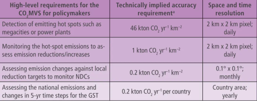
involved in atmospheric GHG measurements and flux estimation (e.g., Le Quéré et al. 2018). From 2023 onward, the IPCC is expected to provide important input to the review of the na-tional GHG inventories at the biennial Facilitative Multilateral Considerations of Progress (FMCP) or the 5-yearly Global Stocktake (GST). Responding to the policy impetus at national, European Union (EU), and global scales, an expert panel from the European Commission (EC) (Pinty et al. 2019) identified the high-level needs of Table 1 that have been translated into technical requirements.

Responsibilities and commitments are not only taken at the governmental level, but also by cities (e.g., the Covenant of Mayors), power plant operators, oil/gas multinationals, and more. Multilevel governance schemes, involving municipal, regional, and national authorities, ask for GHG monitoring, not only with annual national totals, but also with spatiotemporally resolved emissions. The tracking of emission reductions, as intended under the Nationally Determined Contributions (NDC), is facilitated by higher spatial resolution. As shown for air pollutants, the Convention of Long-Range Transboundary Air Pollution (UNECE-CLRTAP 2013) imposed from 2014 onward that Parties report emissions (including point sources) on spatial grids.

Five building blocks of the anthropogenic CO₂ emissions Monitoring and Verification Support (CO₂MVS) capacity

Through the CO₂ Monitoring Task Force, the EC elaborated the space- and ground-based elements for an operational capacity, the so-called CO₂MVS, to monitor and verify anthro-pogenic CO₂ emissions with observation-based evidence in support of climate policymakers. The policy needs of Table 1 require the quantification of the anthropogenic GHG emissions at high spatiotemporal resolution. The CO₂MVS capacity focuses initially on the major con-tribution of the fossil fuel combustion emissions of CO₂ (ffCO₂), and then expands to include other human activities3 _{and other GHGs (e.g., CH}

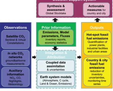
4). Figure 1 shows a schematic diagram of the

functional architecture of the fully integrated CO₂MVS capacity that includes five building blocks: prior information, observa-tions (spaceborne and in situ), integration processes, output/ results, and decision support.

In a first exploratory phase, this CO₂MVS architecture was

outlined by Ciais et al. (2015) and further elaborated in Pinty et al. (2017). Moreover, it appears in the Integrated Global GHG Information System of the World Meteorological Organization (WMO) (DeCola et al. 2019) and the White Paper of the Community of Earth Observation Satel-lites (CEOS) (Crisp et al. 2018). In December 2019, the EC agreed under the Green Deal to start the implementation phase of this CO₂MVS with the Directorate-General Climate Action (DG CLIMA) and EU Member States as main policy users.

GHG emission invento-ries as prior

informa-tion. With the creation

of the UNFCCC came the request for bottom-up emission inventories, es-pecially of Annex-I coun-tries, which were histori-cally contributing the most to the cumulative emissions. The bottom-up accounting of ffCO₂

Table 1. High-level policy needs as identified by Pinty et al. (2017). High-level requirements for the

CO2MVS for policymakers

Technically implied accuracy requirementa

Space and time resolution

Detection of emitting hot spots such as

megacities or power plants 46 kton CO2 yr–1 km–2

2 km x 2 km pixel; daily Monitoring the hot-spot emissions to

as-sess emission reductions/increases 1 kton CO2 yr–1 km–2

2 km x 2 km pixel; daily Assessing emission changes against local

reduction targets to monitor NDCs 0.2 kton CO2 yr–1 km–2

0.1° x 0.1°; monthly Assessing the national emissions and

changes in 5-yr time steps for the GST 0.2 kton CO2 yr–1 per country

Country area; yearly a _{First-order estimate from the Pinty et al. (2017) report.}

3 _{In particular the CO}

2 sources and sinks of

agri-culture, forestry, and land use (AFOLU).

emissions requires rigorous en-ergy statistics, which are based on monthly and annual fuel stock exchanges with a closed balance at global and annual scales. With surveys and mea-surements, the oxygenation factor and the net caloric value for each fuel type were quanti-fied and ffCO₂ emissions were computed. The PA Rulebook, published at the end of 2018, explained how the GST of 2023 will be undertaken with the in-ventories of the emissions from anthropogenic activities occur-ring duoccur-ring 2021. High-quality inventories (with uncertainties ≤3%) are not available for all countries (Janssens-Maenhout et al. 2019).4

Regional differences in pro-cessing model-ready input emis-sion grid maps, subsequently used as prior information, can influence model results, as il-lustrated by Pouliot et al. (2012). More recently for CO₂, Wang et al. (2019) proposed an algorithm

to aggregate grid cells of similar emission fluxes and define a “clump” of area and point sources emitting plumes that will be observable by the current generation of spaceborne sensors, Nassar et al. (2013) emphasized the need to include temporal variations of urban emissions, and Brunner et al. (2019) highlighted the importance of the injection height and velocity of the CO₂ emissions from power plants and industrial facilities.

Atmospheric observations and auxiliary data.

Spaceborne obServationS. The European Environmental

Satel-lite (ENVISAT), 2002–12, was a pioneering spaceborne mission with various instruments measuring the concentration of many atmospheric species. The Scanning Imaging Absorption Spec-trometer for Atmospheric Cartography (SCIAMACHY)

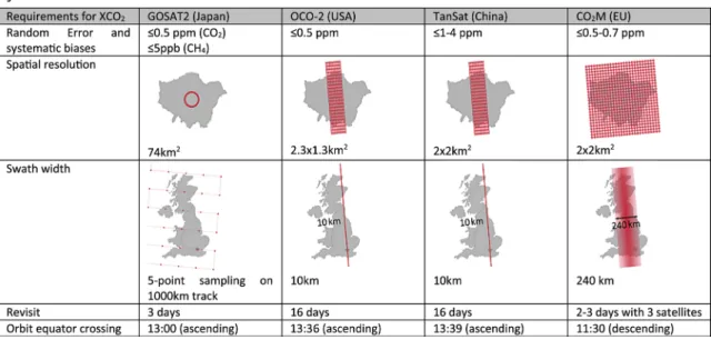
instru-ment measured, among others, GHGs, such as the column-averaged dry-air mole fractions of CO₂ and CH₄, denoted XCO₂ and XCH₄ (e.g., Schneising et al. 2013; Buchwitz et al. 2015, 2018). Since 2009, the Japanese Greenhouse Gases Observing Satellite (GOSAT) with the thermal and near-infrared Fourier transform spectrometer for carbon observations and a cloud and aerosol imager has also been delivering XCO₂ and XCH₄ products (Yoshida et al. 2013; Crisp et al. 2012; Buchwitz et al. 2015). GOSAT-2 was launched in 2018 with considerably improved concentration measurement (see Table 2).

NASA’s Orbiting Carbon Observatory 2 (OCO-2), including a three-channel imaging grat-ing spectrometer, started delivergrat-ing XCO₂ data with an unprecedented high signal-to-noise

Fig. 1. Schematic overview of the planned anthropogenic CO₂MVS

ca-pacity: prior information with first best estimate of the GHG emission inventories and their uncertainties (green, discussed in “GHG emission inventories as prior information”), observations with spaceborne, in situ, auxiliary data including meteorology data (dark blue, discussed in “Atmospheric observations and auxiliary data”), integration and attribu-tion processes with a core model (light blue, discussed in “Integraattribu-tion and attribution system”), the output with consolidated results (yellow, discussed in “Output of the models”), and the decision support process with actionable information for policy-makers (purple, discussed in “Deci-sion support tool with a posteriori evaluation of the GHG inventories”). Data-focused components have a full border, whereas process-focused components have a dashed border.

4 _{Uncertainties for national fossil fuel emission}

inventories range between 3% and 10% for dif-ferent countries (Olivier et al. 2016).

ratio in 2014. The instrument yields the spatial structure of XCO₂ variations across megacities (Schwandner et al. 2017) and allows quantification of ffCO₂ plumes from individual power plants (Nassar et al. 2017). China’s carbon dioxide–monitoring satellite TanSat, launched in late 2016 with an atmospheric CO₂ grating spectrometer, may add another XCO₂ data stream in the near future.

A constellation of European low-Earth-orbit (LEO) CO₂ satellite imagers (CO₂M) are now committed by the EC under the aegis of the Copernicus program, with the main objective to contribute significantly to the policy needs of Table 1 by increasing high-quality satellite observations of XCO₂. The European Space Agency (ESA) leads the design of these CO₂M LEOs with a broad-swath imaging grating spectrometer for CO₂, CH₄, NO₂, and aerosols and plans to deliver science data from January 2026 onward. The main technical specifications of the CO₂M spectrometer,5 _{as described in detail in ESA’s (2019) mission requirements document}

v2.0, are summarized in Table 2 and compared to those of other, currently active sensors. The rationale for collocated observations of NO₂ is to better identify the location and shape of the CO₂ plumes. This takes advantage of the signal-to-noise ratio for NO₂ enhancements, which is much larger than for CO₂ and not contaminated by biospheric emissions. Kuhlmann et al. (2019) demonstrated that auxiliary NO₂ measurements6 _{greatly enhance the detection}

capability for ffCO₂-plume locations. Collocated regional enhancements of XCO₂ observed by

OCO-2 and NO₂ from the Sentinel-5 Precursor (S5P) satellite have already been used by Reuter et al. (2019) to estimate ffCO₂-plume cross-sectional fluxes and to assess the usefulness of simultaneous satellite observations of NO₂ and XCO₂. Auxiliary

aerosol measurements are used to account for perturbations in the optical path of the CO₂ sensor due to aerosol scattering (Frankenberg et al. 2012).7

inSitumeaSurementS. The envisioned CO₂MVS requires in situ

observations for the following purposes:

1) To calibrate and validate the space component that will consist

of column-integrated CO₂ measurements from the ground to the top of the atmosphere. This can be based on the global TCCON8

network, comprising large, upward-looking Bruker sun

Table 2. Comparison of the technical specifications of the Copernicus CO2M satellite to some

cur-rently available sensors (with input of Buchwitz et al. 2018). A constellation of three CO₂M satellites by 2026 is considered.

5 _{Auxiliary instruments on the same platform}

of the Copernicus CO2M satellite include a NO2

spectrometer, a multiangle polarimeter, and a cloud imager.

6 _{Rather than CO as tracer of incomplete fossil}

fuel combustion.

7 _{For local sources such as power plants, CH} 4

measurements support the accuracy of satellite-retrieved XCO2 through the proxy retrieval

method (Frankenberg et al. 2005).

8 _{Total Carbon Column Observing Network}

(http://tccon.caltech.edu/).

spectrometers, supplemented by a similar network of smaller instruments, COCCON.9 _Under

clear-sky conditions, these data can be used after conversion using the WMO-standard mole fraction CO₂ scale (Tans 2009). Collocated vertical CO₂ profile measurements are required to calibrate XCO₂ data from upward-looking spectrometers. Such profiles can be acquired using regular air-core measurements (Karion et al. 2010) and/or using alternatives such as vertical CO₂ profiles collected by regional aircraft.10

2) As a backbone network providing high-quality controlled, homogeneous surface-layer observations

(with expanded spatiotemporal coverage). In Europe, the in situ measurements are coordinated

by ICOS.11 _{Currently, the ICOS network is not homogeneously distributed and provides samples}

biased toward rural locations, focusing more on biospheric than anthropogenic fluxes. Con-sequently, the current network configuration does not sufficiently constrain ffCO₂ estimates. 3) Expansions of coordinated and interoperable urban in situ CO₂ networks, including

observa-tions of 14_{C and other additional tracers. Measuring} 14_{C concentrations in atmospheric CO} 2

is the best approach identified so far for separating ffCO₂ from the natural fluxes because fossil fuels do not contain 14_{C (Levin et al. 2003; Turnbull et al. 2006). Observations of} 14_C

and ffCO₂ co-emitted species across major ffCO₂ emitting regions will provide complemen-tary information to satellites for quantifying anthropogenic emissions from hot spots and for attributing the large-scale CO₂ signal.

The CO₂MVS spans a range of scales, from large point sources to country scales, which adds additional requirements for the in situ component: denser networks of sun spec-trometers, denser continental-scale networks of ground-based CO₂, tracers and 14_{C and}

portable instruments and local/regional CO₂ networks around selected hot spot areas for city-scale and large industrial complexes to validate the gradients up and downwind of the emitting sources. International coordination and standardization by WMO12 _and

sus-tained operational and scientific funding are recommended for a successful implementation of the CO₂MVS capacity by Pinty et al. (2019).

meteorological and other auxiliary data. Meteorology is

an important driver for the natural carbon cycle, and meteo-rological fields can be used as a proxy for the spatiotemporal distribution of temperature-dependent anthropogenic emis-sions.13 _{In addition, meteorological data are key to constrain the}

atmospheric transport that links the observed atmospheric GHG concentrations and the actual emissions. The foreseen CO₂MVS capacity can fully benefit here from the heritage of numerical weather prediction (NWP), with its operational data-exchange mechanisms, and developments are well underway for a global high-resolution CO₂ ensembles-based system (Agustí-Panareda et al. 2019; McNorton et al. 2020).

In addition, FLUXNET,14 _{a global network of eddy covariance}

measurements of CO₂ and H₂O exchange fluxes between the Earth and the atmosphere, can provide important independent data. Similarly, observations of other trace gases and particulate matter co-emitted with CO₂ can help identify spatiotemporal distribution of ffCO₂ emission sources. Some constituents are already monitored for air quality purposes (e.g., AERONET,15

EIONET16 _{for aerosols) and temporal profiles are devised in air}

quality models (e.g., Denier van der Gon et al. 2011).17

9 _{Collaborative Carbon Column Observing Network}

(https://www.imk-asf.kit.edu/english/3221.php).

10 _{With passenger aircraft CO}

2 profiles [e.g., the

IAGOS (https://www.iagos.org/) and CONTRAIL (www.cger.nies.go.jp/contrail/contrail.html-initiatives)] collocation of sun spectrometers is not achieved today and will require an extension of the TCCON and COCCON networks around airports.

11 _{Integrated Carbon Observation System}

(https://www.icos-ri.eu/).

12 _{For example, via the Global Atmosphere Watch}

(www.wmo.int/pages/prog/arep/gaw/gaw_home _en.html).

13 _{For example, heating degree-days for the}

distri-bution of the residential heating emissions.

14 _{About 40 micrometeorological tower sites,}

included in the FLUXNET infrastructure, are measuring CO2 emissions in urban areas

(http://fluxnet.fluxdata.org/).

15 _{Aerosol Robotic Network is a federation of}

ground-based remote sensing aerosol networks (https://aeronet.gsfc.nasa.gov/).

16 _{European Environment Information and}

Obser-vation Network.

17 _{As selected for being implemented in the}

Coper-nicus Atmosphere Monitoring Service.

Integration and

attribu-tion system. The

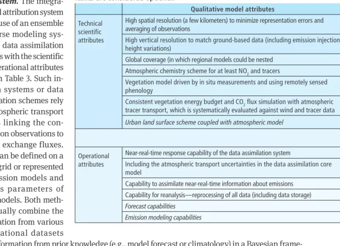
integra-tion and attribuintegra-tion system makes use of an ensemble of inverse modeling sys-tems or data assimilation schemes with the scientific and operational attributes listed in Table 3. Such in-version systems or data assimilation schemes rely on atmospheric transport models linking the con-centration observations to surface exchange fluxes. These can be defined on a model grid or represented by emission models and process parameters of these models. Both meth-ods usually combine the information from various observational datasets

with information from prior knowledge (e.g., model forecast or climatology) in a Bayesian frame-work, i.e., by minimizing a cost function that takes the uncertainties of all the datasets into account. Estimates of the model errors are accounted for by combining them to the observational uncertainties or through the use of model ensembles.18 _{Examples for a gridded inversion}

system can be found in Basu et al. (2013) or Gaubert et al. (2019) and for a process-based scheme in T. Kaminski et al. (2020, manuscript submitted to

Nat. Commun.). Both approaches require consistency between

all input datasets (preferably steered with a realistic prior) or a bias correction within the data assimilation system itself (e.g., Dee and Uppala 2009).19 _{Earth observations are a key driver}

for Earth system modeling developments (Balsamo et al. 2018) representing natural and human-induced disturbances in the water, energy, and carbon cycle at the surface that are affecting CO₂ fluxes.

Super et al. (2017) explored the need for plume modeling to

understand point sources in an urban-industrial complex, under the impact of different scales of meteorology. Experience with plume modeling has been gained mainly by the air quality community (e.g., Leelőssy et al. 2014) but also by the CO₂ community (e.g., Kuhlmann et al. 2019; Nassar et al. 2017). Although the long-lived CO₂ plume, with relatively small enhance-ment over the ambient background, diffuses differently from the plume of a short-lived NO₂ air pollutant, with relative high concentration enhancement in the atmosphere, both plumes show similar structures and the NO₂ plume is a good marker of the CO₂ plume. For the plume or puff modeling, there is know-how available from dispersion studies of (radioactive) air pollution. The modeling strategy for the CO₂MVS capacity combines different scales, from global to local, in order to cover ultimately the NDCs over a region/country. Figure 2 illustrates the challenge to link the local CO₂ flux footprint region of the in situ observations with the country scale of the national inventories and NDCs.

Table 3. Scientific and operational attributes of the core models. The attributes in italics are considered optional.

Qualitative model attributes

Technical scientific attributes

High spatial resolution (a few kilometers) to minimize representation errors and averaging of observations

High vertical resolution to match ground-based data (including emission injection height variations)

Global coverage (in which regional models could be nested Atmospheric chemistry scheme for at least NO₂ and tracers

Vegetation model driven by in situ measurements and using remotely sensed phenology

Consistent vegetation energy budget and CO2 flux simulation with atmospheric tracer transport, which is systematically evaluated against wind and tracer data

Urban land surface scheme coupled with atmospheric model

Operational attributes

Near-real-time response capability of the data assimilation system

Including the atmospheric transport uncertainties in the data assimilation core model

Capability to assimilate near-real-time information about emissions Capability for reanalysis—reprocessing of all data (including data storage)

Forecast capabilities

Emission modeling capabilities

18 _{This is also envisaged in the Community}

Inver-sion Framework (CIF), under development in the H2020 project VERIFY (see section “Way forward and challenges ahead”).

19 _{The various input data streams are then bias}

corrected to a common baseline, which is defined by a dataset with high accuracy and precision.

Output of the models. Output of the CO₂MVS will address a variety of spatiotemporal scales and various user communities.

At the global level, the GST is in line with the implementation of the PA. In 2028 the CO₂MVS capacity should help evaluating the bottom-up GHG estimates and their difference with respect to 2023, assessing the effectiveness of the reductions of the NDCs.

At the country level, the CO₂MVS needs to support the review of country budgets and to quantify through rigorous uncertainty propagation the impact of additional observational information into an uncertainty reduction in inferred emission fields [as illustrated for CH₄ by Bergamaschi et al. (2010)].

At the level of substate actors, such as cities or industrial complexes, the spatiotemporal

view on the emissions might reveal insights on the effectiveness of initiatives related to, e.g., carbon trading, greening of cities, and others. This new area of applications is where a significant contribution of an observation-driven operational CO₂MVS can be expected.

Decision support tool with a posteriori evaluation of the GHG inventories. An important

spin-off from the CO₂MVS could be the provision of an assessment tool, open to UNFCCC and its Parties for monitoring NDC implementation worldwide. This still demands significant studies to determine the trends expected from the implementation of the NDCs, and more specifically where, when, and at what rate these trends are occurring. Most likely one of the robust results of a space-based observation system will be the monitoring of XCO₂ trends and change in posterior emission fluxes over multiple years. These results will yield spatiotempo-ral resolutions higher than possible on the sole basis of the national inventories and should provide evidence for tracking progress toward the NDCs’ reduction targets. Moreover, maps of uncertainty reductions will inform where extra efforts such as additional measurements and/or more accurate GHG accounting infrastructures would best reduce the ffCO₂-budget uncertainty.

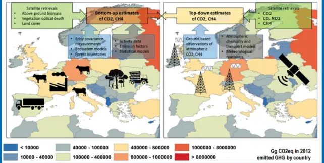
Fig. 2. Interplay between (left) bottom-up estimates (based on human activity data) and (right) top-down estimates (based on spaceborne or in situ observations) in the modeling chain, covering different scales from global to local. Obviously, it is challenging to monitor and verify a country’s annual inventory (represented by the colored patchwork over Europe) based on atmospheric observations over time.

Long-term operations with an institutional framework consolidated by international collaboration

To develop the operational CO₂MVS capacity, the EC coordinates efforts from three major Eu-ropean institutions—ESA for developing the space segment, the EuEu-ropean Organisation for the Exploitation of Meteorological Satellites (EUMETSAT) for operating the space segment, and the European Centre for Medium-Range Weather Forecasts (ECMWF)—for providing the modeling capacity required to integrate the overall observations. The initiative builds on existing modeling infrastructures, includes the design of a series of unprecedented satellite and ground-based CO₂ and CH₄ observation systems, and capitalizes on model-based analysis. EUMETSAT and ESA define the system requirements (for the space segment, the operations, and the ground segment) and take care of the operation of the satellite with continuous calibration/validation and data transmission. EUMETSAT foresees full automatic dissemina-tion of the geophysical product data at native instrument resoludissemina-tion within 48 h, such that ECMWF and its partners with full model setup can provide a Copernicus CO₂ service with quasi-near-real-time products.

After calibration and operational tests of the CO₂MVS capacity over selected European countries, it will be possible to apply the CO₂MVS globally. The global applications, for re-gions outside Europe, will require extra in situ data, whose availability and access should be fostered by international collaborations. The EC and the relevant European institutional partners are already engaged bilaterally and multilaterally with international organizations20

for the strategic, policy-relevant, and technical dimensions related to the setup of a global CO₂ monitoring capacity.

Way forward and challenges ahead

Monitoring of the anthropogenic CO₂ emissions in a consistent and systematic manner for all countries enables the identification of sources that can be further reduced in the GST assess-ments. This monitoring requires continuity of knowledge and data with sufficient spatiotem-poral coverage, because of the significant and expectedly increasing variability of emission sources (e.g., with the renewables progressively replacing the fossil fuels). Quantification of the CO₂ plumes from power plants remains challenging, in particular when they are located in morphologically complex areas, such as near coastlines.

Industrial complexes and urban areas add another level of heterogeneity and complexity to the plumes to be monitored. Various aspects of the challenges faced in building up the CO₂MVS capacity are discussed in the so-called “blue”, “red,” and “green” reports of the EC with a series of recommendations for actions.

Figure 3 sketches the planned development of the CO₂MVS and highlights the main milestones including the research components, namely:

The ESA and EUMETSAT support studies21 _{provide first input}

to the satellite system and product processing design, the product continuous calibration/validation and monitoring, and conclude with the need for collocated measurements of NO₂ and aerosols (with both an NO₂ spectrometer and a multi-angle polarimeter on the CO₂M platform). The spatiotemporal coverage with a series of constellation configurations as well as the impact of the technical parameter ranges have been estimated using well-defined assumptions.

20 _{For example, WMO, Committee on Earth}

Observa-tion Satellites (CEOS), and CoordinaObserva-tion Group for Meteorological Satellites (CGMS).

21 _{Carbon Cycle Fossil Fuel Data Assimilation}

Sys-tem (CCFFDAS); Poor Man’s Inversion Framework (PMIF); Satellite Measurements of Auxiliary Reac-tive Trace Gases for Fossil Fuel Carbon Dioxide Emission Estimation (SMARTCARB); Study on Use of Aerosol Information for Estimating Fossil Fuel CO2 Emissions (AEROCARB); spectral sizing

study; error budget study; E2F Simulator; system and instrumentation predevelopment; Airborne Carbon Dioxide Imager for Atmosphere (ACA-DIA); GHG product processing and continuous calibration/validation requirements definition; level 1 processing requirements for CO2

monitor-ing mission; definition of requirements for an integrated function for calibration, validation, and monitoring of level 1 and level 2 products for CO2 monitoring mission; top-of-atmosphere

simulations for the evaluation of data processing for the CO2 monitoring mission..

The H2020 projects CHE22 _{and VERIFY}23 _{prepare for an improved modeling and data}

assimi-lation, quantifying more accurately fluxes of CO₂ and CH₄ across Europe with enhanced, more detailed emission inventories, separating the anthropogenic and natural emission components and their drivers by advanced modeling and

accurate characterization of the space–time variations of GHG fluxes.

Since 2015, the feasibility of the CO₂MVS has been explored. This phase is now successfully concluded with the go-ahead for the concrete phase of implementation and integration. The UNFCCC-SBSTA (2019) recognized the full system approach for monitoring CO₂ and CH₄ from space, combining satellite, in situ, and modeling components for emission estimates and

encouraging Parties to the Convention to engage the necessary resources and competence to this endeavor. At a more public outreach level, it is also true that the visualization of the

Fig. 3. Timeline for the development of a European operational GHG Monitoring and Verification Support capacity with the exploratory phase, the implementation/integration phase, and the operational phase. The exploratory phase is concluded with the reports of the CO₂ Monitoring Task Force [the blue CO₂ report of Ciais et al. (2015), the red CO₂ report of Pinty et al. (2017), and the green CO₂ report of Pinty et al. (2019)], the Mission Requirements Document (MRD) of ESA (versions 1.0 and 2.0), and the CEOS white paper of Crisp et al. (2018). In the exploratory phase, different Research and Development studies have been launched by the EC (under the Horizon

2020 Research Framework program), ESA, and EUMETSAT in support of the CO₂MVS design (green

arrow). In addition, ESA and EUMETSAT launched studies to further develop the space component (orange arrow) and the ground segment (purple arrow), respectively.

22 _{CHE stands for CO}

2 Human Emissions and is the

H2020 coordination support action project of the EC (https://che-project.eu/).

23 _{VERIFY stands for Observation-Based}

Monitor-ing and Verification of Greenhouse Gases and is a H2020 scientific research project of the EC (https://verify.lsce.ipsl.fr/)

CO₂ emissions might be part of the more general solution to call for urgent climate action in implementing the PA.

We have a clear understanding of the CO₂MVS, and the system architecture implementa-tion, although challenging, is within the means of EC, ESA, EUMETSAT, and ECMWF and the necessary coordination mechanisms. The timeline for implementation is demanding but well defined, and the system is expected to provide from 2026 onward pre-operational outputs and insight, by visualizing CO₂ emission plumes, and in particular the effects of non-implemented reductions, globally. As the CO₂MVS will have been calibrated over Europe, collaboration with our international partners is being actively pursued since the beginning to make the best out of the observations outside Europe as well.

Acknowledgments.Studies are conducted in preparation for a European capacity to monitor

CO₂ anthropogenic emissions under the Coordination and Support Action H2020-EO-3-2017 with project CHE (CO₂ Human Emissions) and under the Research and Innovation Action H2020-SC5-4-2017 with project VERIFY (Observation-based monitoring and verification of greenhouse gases). The CHE and VERIFY projects have received funding from the European Union’s Horizon 2020 research and innovation program under Grant Agreements 776186 and 776810, respectively.

References

Agustí-Panareda, A., and Coauthors, 2019: Modelling CO₂ weath-er—Why horizontal resolution matters. Atmos. Chem. Phys.,

19, 7347–7376, https://doi.org/10.5194/acp-19-7347-2019.

Balsamo, G., and Coauthors, 2018: Satellite and in situ observa-tions for advancing global earth surface modelling: A review.

Remote Sens., 10, 2038, https://doi.org/10.3390/rs10122038.

Basu, S., and Coauthors, 2013: Global CO₂ fluxes estimated from GOSAT retrievals of total column CO₂. Atmos. Chem. Phys.,

13, 8695–8717, https://doi.org/10.5194/acp-13-8695-2013.

Bergamaschi, P., and Coauthors, 2010: Inverse modeling of Eu-ropean CH₄ emissions 2001–2006. J. Geophys. Res., 115, D22309, https://doi.org/10.1029/2010JD014180.

——, and Coauthors, 2018: Atmospheric monitoring and inverse modelling for verification of greenhouse gas inventories. Pub-lications Office of the European Union, 109 pp., https://doi .org/10.2760/759928.

Brunner, D., G. Kuhlmann, J. Marshall, V. Clément, O. Fuhrer, G. Bro-quet, A. Löscher, and Y. Meijer, 2019: Accounting for the verti-cal distribution of emissions in atmospheric CO₂ simulations.

Atmos. Chem. Phys., 19, 4541–4559, https://doi.org/10.5194

/acp-19-4541-2019.

Buchwitz, M., and Coauthors, 2015: The Greenhouse Gas Climate Change Initiative (GHG-CCI): Comparison and quality as-sessment of near-surface-sensitive satellite-derived CO₂ and CH₄ global data sets. Remote Sens. Environ., 162, 344–362, https://doi.org/10.1016/j.rse.2013.04.024.

——, and Coauthors, 2018: Copernicus Climate Change Service (C3S) global satellite observations of atmospheric carbon di-oxide and methane. Adv. Astronaut. Sci. Technol., 1, 57–60, https://doi.org/10.1007/s42423-018-0004-6.

Ciais, P., D. Crisp, H. Denier Van Der Gon, R. Engelen, M. Heimann, G. Janssens-Maenhout, P. Rayner, and M. Scholze, 2015: To-wards a European Operational Observing System to Monitor Fossil CO₂ Emissions. European Commission Joint Research Centre, 65 pp., https://doi.org/10.2788/350433.

Crisp, D., and Coauthors, 2012: The ACOS CO₂ retrieval algo-rithm—Part II: Global XCO₂ data characterization. Atmos.

Meas. Tech., 5, 687–707, https://doi.org/10.5194/amt-5-687

-2012.

——, and Coauthors, 2018: A constellation architecture for moni-toring carbon dioxide and methane from space. CEOS Atmo-spheric Composition Virtual Constellation Greenhouse Gas Team Rep., 173 pp., http://ceos.org/document_management/ Virtual_Constellations/ACC/Documents/CEOS_AC-VC_GHG _White_Paper_Version_1_20181009.pdf.

DeCola, P., O. Tarasova, and IG2IS Science Team, 2019: The in-tegrated global GHG information system science team, the integrated global GHG information system first user sum-mit. Geophysical Research Abstracts, Vol. 21, Abstract 18026, https://meetingorganizer.copernicus.org/EGU2019/EGU2019 -18026.pdf.

Dee, D., and S. Uppala, 2009: Variational bias correction of sat-ellite radiance data in the ERA-Interim reanalysis. Quart. J.

Roy. Meteor. Soc., 135, 1830–1841, https://doi.org/10.1002

/qj.493.

Denier van der Gon, H., C. Hendriks, J. Kuenen, A. Segers, and A. Visschedijk, 2011: Description of current temporal emission patterns and sensitivity of predicted AQ for temporal emis-sion patterns. TNO Rep. EU FP7 MACC Deliverable Rep. D_D-EMIS_1.3, 22 pp., https://atmosphere.copernicus.eu/sites /default/files/2019-07/MACC_TNO_del_1_3_v2.pdf.

DG CLIMA, 2014: A policy framework for climate and energy in the period from 2020 to 2030. COM(2014)15final. Di-rectorate General Climate Action of the European Com-mission, 18 pp., https://eur-lex.europa.eu/legal-content/EN /ALL/?uri=CELEX%3A52014DC0015.

ESA, 2019: Copernicus CO₂ Monitoring Mission Requirements Document. EOP-SM/3088/YM-ym, 82 pp., https://esamul-timedia.esa.int/docs/EarthObservation/CO2M_MRD_v2.0 _Issued20190927.pdf.

Frankenberg, C., J. F. Meirink, M. Van Weele, U. Platt, and T. Wag-ner, 2005: Assessing methane emissions from global space-borne observations. Science, 308, 1010–1014, https://doi .org/10.1126/science.1106644.

——, O. Hasekamp, C. O’Dell, S. Sanghavi, A. Butz, and J. Worden, 2012: Aerosol information content analysis of multi-angle high spectral resolution measurements and its benefit for high accuracy greenhouse gas retrievals. Atmos. Meas. Tech.,

5, 1809–1821, https://doi.org/10.5194/amt-5-1809-2012.

Gaubert, B., and Coauthors, 2019: Global atmospheric CO₂ inverse models converging on neutral tropical land exchange, but dis-agreeing on fossil fuel and atmospheric growth rate.

Biogeosci-ences, 16, 117–134, https://doi.org/10.5194/bg-16-117-2019.

IPCC, 2006: 2006 IPCC Guidelines for National Greenhouse Gas Inventories. S. Eggleston et al., Eds., IPCC, www.ipcc-nggip .iges.or.jp/public/2006gl/.

Janssens-Maenhout, G., and Coauthors, 2019: EDGAR v4.3.2 Global Atlas of the three major greenhouse gas emissions for the period 1970–2012. Earth Syst. Sci. Data, 11, 959–1002, https://doi.org/10.5194/essd-11-959-2019.

Kaminski, T., and Coauthors, 2020: Atmospheric CO₂ observations from space can support national inventories. Nat. Commun., submitted.

Karion, A., C. Sweeney, P. Tans, and T. Newberger, 2010: Air-Core: An innovative atmospheric sampling system. J.

Atmos. Oceanic Technol., 27, 1839–1853, https://doi

.org/10.1175/2010JTECHA1448.1.

Kuhlmann, G., G. Broquet, J. Marshall, V. Clement, A. Löscher, Y. Mei-jer, and D. Brunner, 2019: Detectability of CO₂ emission plumes of cities and power plants with the Copernicus Anthropogenic CO₂ Monitoring (CO2M) mission. Atmos. Meas. Tech., 12, 6695–6719, https://doi.org/10.5194/amt-12-6695-2019. Leelőssy, A., F. Molnar Jr., F. Izsak, A. Havasi, I. Lagzi, and R.

Meszaros, 2014: Dispersion modelling of air pollutants in the atmosphere: A review. Cent. Eur. J. Geosci., 6, 257–278, https://doi.org/10.2478/s13533-012-0188-6.

Le Quéré, C., and Coauthors, 2018: Global carbon budget 2017.

Earth Syst. Sci. Data, 10, 405–448, https://doi.org/10.5194

/essd-10-405-2018.

Levin, I., B. Kromer, M. Schmidt, and H. Sartorius, 2003: A novel approach for independent budgeting of fossil fuel CO₂ over Europe by 14CO2 observations. Geophys. Res. Lett., 30, 2194, https://doi.org/10.1029/2003GL018477.

McNorton, J., and Coauthors, 2020: Representing model uncer-tainty for global atmospheric CO₂ flux inversions using EC-MWF-IFS-46R1. Geosci. Model Dev., 13, 2297–2313, https:// doi.org/10.5194/gmd-13-2297-2020.

Nassar, R., L. Napier-Linton, K. R. Gurney, R. J. Andres, T. Oda, F. R. Vogel, and F. Deng, 2013: Improving the temporal and spatial distribution of CO₂ emissions from global fossil fuel emission data sets. J. Geophys. Res. Atmos., 118, 917–933, https://doi .org/10.1029/2012JD018196.

——, T. G. Hill, C. A. McLinden, D. Wunch, B. A. Jones, and D. Crisp, 2017: Quantifying CO₂ emissions from individual power plants from space. Geophys. Res. Lett., 44, 10 045–10 053, https://doi.org/10.1002/2017GL074702.

Olivier, J. G. J., G. Janssens-Maenhout, M. Muntean, and J. A. H. W. Peters, 2016: Trends in global CO₂ emissions: 2016 report. JRC 103425, 82 pp., https://edgar.jrc.ec.europa.eu/news_docs/jrc-2016-trends-in-global-co2-emissions-2016-report-103425.pdf. Peters, G. P., and Coauthors, 2017: Towards real-time verification

of CO₂ emissions. Nat. Climate Change, 7, 848–850, https:// doi.org/10.1038/s41558-017-0013-9.

Pinty B., and Coauthors, 2017: An operational anthropogenic CO₂ emissions monitoring and verification support capacity: Base-line requirements, model components and functional architec-ture. European Commission Joint Research Centre, EUR 28736 EN, 98 pp., https://doi.org/10.2760/08644.

——, and Coauthors, 2019: An operational anthropogenic CO₂ emissions monitoring and verification support capacity: Needs and high level requirements for in situ measurements. European Commission Joint Research Centre, EUR 29817 EN, 72 pp., https://doi.org/10.2760/182790.

Pouliot, G., T. Pierce, H. Denier van der Gon, M. Schaap, and U. Nopmongcol, 2012: Comparing emissions inventories and model-ready emissions datasets between Europe and North America for the AQMEII project. Atmos. Environ., 53, 4–14, https://doi.org/10.1016/j.atmosenv.2011.12.041.

Reuter, M., M. Buchwitz, O. Schneising, S. Krautwurst, C. W. O’Dell, A. Richter, H. Bovensmann, and J. P. Burrows, 2019: Towards monitoring localized CO₂ emissions from space: Co-located regional CO₂ and NO₂ enhancements observed by the OCO-2 and S5P satellites. Atmos. Chem. Phys., 19, 9371–9383, https://doi.org/10.5194/acp-19-9371-2019.

Schneising, O., J. Heymann, M. Buchwitz, M. Reuter, H. Bovens-mann, and J. P. Burrows, 2013: Anthropogenic carbon dioxide source areas observed from space: Assessment of regional en-hancements and trends. Atmos. Chem. Phys., 13, 2445–2454, https://doi.org/10.5194/acp-13-2445-2013.

Schwandner, F. M., and Coauthors, 2017: Spaceborne detection of localized CO₂ sources. Science, 358, eaam5782, https://doi .org/10.1126/SCIENCE.AAM5782.

Super, I., H. A. C. Denier van der Gon, M. K. van der Molen, H. A. M. Sterk, A. Hensen, and W. Peters, 2017: A multi-model ap-proach to monitor emissions of CO₂ and CO from an urban– industrial complex. Atmos. Chem. Phys., 17, 13 297–13 316, https://doi.org/10.5194/acp-17-13297-2017.

Tans, P., 2009: An accounting of the observed increase in oceanic and atmospheric CO₂ and an outlook for the future.

Oceanog-raphy, 22, 26–35, https://doi.org/10.5670/oceanog.2009.94.

Turnbull, J. C., J. B. Miller, S. J. Lehman, P. P. Tans, R. J. Sparks, and J. Southon, 2006: Comparison of 14_CO

2, CO, and SF6 as trac-ers for recently added fossil fuel CO₂ in the atmosphere and implications for biological CO₂ exchange. Geophys. Res. Lett.,

33, L01817, https://doi.org/10.1029/2005GL024213.

UNECE–CLRTAP, 2013: Convention on Long Range Transbound-ary Air Pollution. Decision 2013/3 & 2013/4 ECE/Ab.AIR/122/ Add.1, www.unece.org/env/lrtap/executivebody/eb_decision .html.

UNFCCC, 2015: The Paris Agreement. 25 pp., http://unfccc. int/files/essential_background/convention/application/pdf /english_paris_agreement.pdf.

UNFCCC-SBSTA, 2017: Subsidiary Body for Scientific and Techno-logical Advice, 46th session. FCCC/SBSTA/2017/L.21, 16 pp., https://unfccc.int/resource/docs/2017/sbsta/eng/01.pdf. ——, 2019: Subsidiary Body for Scientific and Technological

Ad-vice, 51st session. FCCC/SBSTA/2019/L.15, 3 pp., https://undocs .org/FCCC/SBSTA/2019/L.15.

Wang, Y., and Coauthors, 2019: A global map of emission clumps for future monitoring of fossil fuel CO₂ emissions from space.

Earth Syst. Sci. Data, 11, 687–703, https://doi.org/10.5194

/essd-11-687-2019.

Witi, J., and D. Romano, 2019: Reporting guidance and tables. 2019 Refinement to the 2006 IPCC Guidelines for Na-tional Greenhouse Gas Inventories, Vol. 1, D. Gomez and W. Irving, Eds., IPCC, 8.1–8.36, www.ipcc-nggip.iges.or.jp/ public/2019rf/pdf/1_Volume1/19R_V1_Ch08_Reporting _Guidance.pdf.

Yoshida, Y., and Coauthors, 2013: Improvement of the retrieval al-gorithm for GOSAT SWIR XCO₂ and XCH₄ and their validation using TCCON data. Atmos. Meas. Tech., 6, 1533–1547, https:// doi.org/10.5194/amt-6-1533-2013.