HAL Id: hal-01781389
https://hal.inria.fr/hal-01781389v2
Submitted on 8 May 2018
HAL is a multi-disciplinary open access
archive for the deposit and dissemination of
sci-entific research documents, whether they are
pub-lished or not. The documents may come from
teaching and research institutions in France or
abroad, or from public or private research centers.
L’archive ouverte pluridisciplinaire HAL, est
destinée au dépôt et à la diffusion de documents
scientifiques de niveau recherche, publiés ou non,
émanant des établissements d’enseignement et de
recherche français ou étrangers, des laboratoires
publics ou privés.
Leveraging the Potential of WSN for an Efficient
Correction of Air Pollution Fine-Grained Simulations
Ahmed Boubrima, Walid Bechkit, Hervé Rivano, Lionel Soulhac
To cite this version:
Ahmed Boubrima, Walid Bechkit, Hervé Rivano, Lionel Soulhac. Leveraging the Potential of WSN
for an Efficient Correction of Air Pollution Fine-Grained Simulations. ICCCN 2018 - 27th
Interna-tional Conference on Computer Communications and Networks, Jul 2018, Hangzhou, China. pp.1-9,
�10.1109/ICCCN.2018.8487343�. �hal-01781389v2�
Leveraging the Potential of WSN for an Efficient
Correction of Air Pollution Fine-Grained
Simulations
Ahmed Boubrima
∗, Walid Bechkit
∗, Hervé Rivano
∗and Lionel Soulhac
†∗Univ Lyon, Inria, INSA Lyon, CITI, F-69621 Villeurbanne, France
†LMFA, Univ Lyon, CNRS UMR 5509 ECL, INSA Lyon, Univ Claude Bernard, 69134 Ecully, France
Abstract—One of the main concerns of smart cities is to improve public health which is mainly threatened by air pollution due to the massively increasing urbanization. The reduction of air pollution starts first with an efficient monitoring of air quality where the main aim is to generate accurate pollution maps in real time. Spatiotemporally fine-grained air pollution maps can be ob-tained using physical models which simulate the phenomenon of pollution dispersion. However, these simulations are less accurate than measurements that can be obtained using pollution sensors. Combining simulations and measurements, also known as data assimilation, provides better pollution estimations through the correction of the fine-grained simulations of physical models. The quality of data assimilation mainly depends on the number of measurements and their locations. A careful deployment of nodes is therefore necessary in order to get better pollution maps. In this paper, we tackle the deployment problem of pollution sensors and propose a new mixed integer programming model allowing to minimize the overall deployment cost of the network while achieving a required assimilation quality and ensuring the connectivity of the network. We then design a heuristic algorithm to solve efficiently the problem in polynomial time. We perform extensive simulations on a dataset of the Lyon city, France and show that our approach provides better air quality monitoring when compared to existing deployment methods that are designed without taking into account the outputs of physical models. We also show that in terms of connectivity, the communication range of sensor nodes might have a noteworthy impact on the quality of pollution estimation.
Keywords— Wireless sensor networks, deployment, air pol-lution simulation, data assimilation.
I. INTRODUCTION
Wireless sensor networks (WSN) are widely used in envi-ronmental applications where the aim is to sense a physical phenomenon such as temperature, humidity, air pollution, etc. In this context of application, the use of WSN allows us to understand the variations of the phenomenon over the monitoring region and therefore be able to take adequate decisions regarding the impact of the phenomenon [1]. Air pollution is one of the main physical phenomena that still need to be studied and characterized because it highly depends on other phenomena such as temperature and wind variations. In addition, air pollution is becoming a major threat to human health in urban environments. According to the World Health Organization (WHO), exposure to air pollution is accountable to seven million casualties in 2012. In 2013, the International Agency for Research on Cancer (IARC) classified particulate
matter, the main component of outdoor pollution, as carcino-genic for humans. Air pollution is therefore considered as a major issue of modern megalopolis, where the majority of world population lives. As a consequence, the effective monitoring of pollutant emissions is at the heart of many sustainable development efforts, in particular those of smart cities.
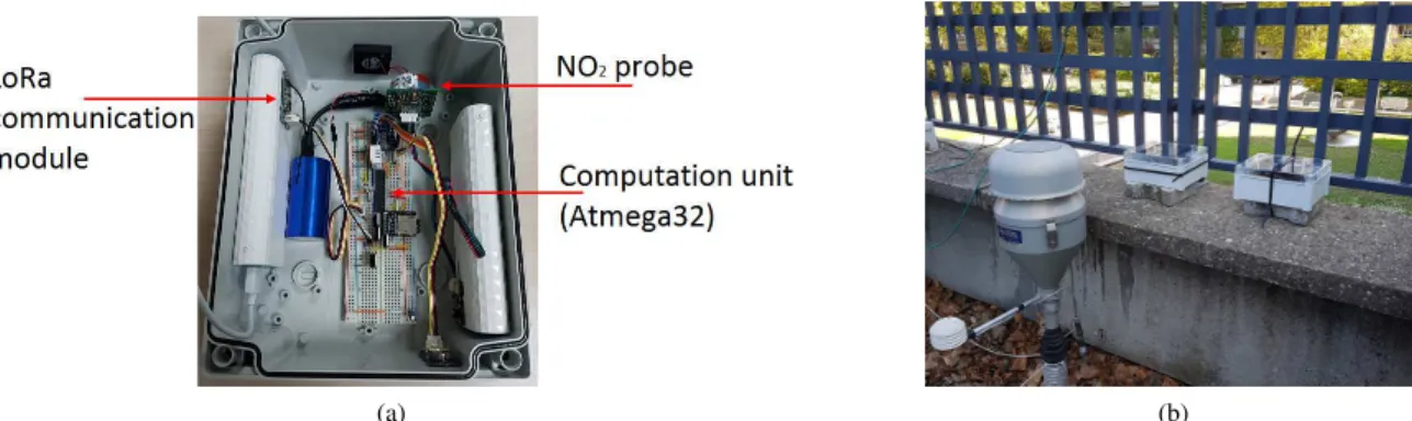
Current air pollution monitoring stations are equipped with multiple lab pollution sensors. These systems are however massive, inflexible and expensive. An alternative – or comple-mentary – solution would be to use wireless sensor networks. The progress of electrochemical sensors, that are smaller and cheaper, makes the use of WSN for air pollution monitoring viable thanks to their reasonable measurement quality (see Fig. 1 for our lab-designed sensors).
The aim of using WSN for air pollution monitoring, also known as air pollution mapping, is usually to generate accurate pollution maps in real time [2]. Unlike the work we presented in [3] where we consider only sensor measurements in the generation of pollution maps, we propose in this work to perform air pollution mapping based on physical models which simulate the phenomenon of pollution dispersion. Our aim is to consider the application case of data assimilation techniques which are used to correct the simulations of physical models based on sensor measurements. In this context, we tackle in this paper the optimal deployment of sensor nodes for an effective data assimilation of air pollution measurements.
The deployment optimization is a major challenge in WSN design. The problem consists in determining the optimal positions of sensors and sinks so as to cover the environment and ensure the network connectivity while optimizing an objective function such as the deployment cost or the network lifetime [4]. The network is said connected if each sensor can communicate information to at least one sink node. As for the coverage issue, it has been often modeled as a k-coverage problem where at least k sensors should monitor each point of interest.
We propose in this paper a deployment approach allowing to minimize the deployment cost of nodes while ensuring a required assimilation quality and the connectivity of the sensor network. Unlike most of the existing deployment approaches, which are either generic or assume that sensors have a given detection range, we base on data assimilation to define an
(a) (b)
Fig. 1: Our nitrogen dioxide (N O2) lab-designed sensors. (a) Internal view of a sensor node. (b) Field deployment of 2 nodes
next to a monitoring station in Lyon, France.
appropriate mathematical formulation of coverage quality in the context of air pollution mapping. We formulate the quality of air pollution mapping of a given sensor network depending on the assimilation error of pollution concentration at locations where no sensor is deployed. The assimilation error is defined as the difference between the ground truth (or real) value of pollution concentration and the concentration obtained by applying an adequate data assimilation method on the mea-surements of sensor nodes and the outputs of physical models. We use our formulation of air quality mapping to define a deployment model using mixed integer linear programming (MILP). Then, we analyze the computational complexity of our optimization model and derive a heuristic algorithm that runs in polynomial time based on linear relaxation.
We perform extensive simulations on a dataset of the Lyon city, France and show that our approach provides better air quality monitoring when compared to existing deployment methods that are designed without taking into account the outputs of physical models. Finally, we show that in terms of connectivity, the communication range of sensor nodes might have a noteworthy impact on the quality of pollution estimation.
The main contributions of this work can be summarized as follows:
1) An adequate mathematical formulation of coverage qual-ity that is based on the combination of pollution simu-lations and sensor measurements.
2) An MILP deployment model designed using lineariza-tion techniques.
3) A heuristic algorithm based on the linear relaxation concept.
4) A comparison to interpolation-based deployment ap-proaches which do not take into account the outputs of physical models.
The remaining of this paper is organized as follows. We first review the related works on the deployment issue of WSN in section II. Then, we present in details our mathematical formulation of coverage quality in section III. Next, we present our optimization model in section IV and discuss the resolution
of the model in section V. After that, we present the simulation data set and analyze the obtained results in section VI. Finally, we conclude the paper and provide some perspectives in section VII.
II. RELATED WORKS: WSNDEPLOYMENT
The deployment issue of wireless sensor networks has been addressed extensively in the literature where several mathematical models, optimal algorithms and near-optimal heuristics have been proposed [5]. The problem has been defined in multiple ways depending on the context of the deployment. The main issues targeted in the literature are coverage, connectivity, network lifetime and the network de-ployment cost. In this section, we identify what lacks in the literature and motivates the need of an application-aware deployment approach toward an effective assimilation of air pollution measurements. We present the related works based on their coverage definition while identifying their formulation of connectivity and network lifetime.
Existing deployment approaches are either event-aware [6] [7] [8] [9] [10] [11] or correlation-aware [12] [13] [14] [15] [16]. In the first case, a sensor is assumed to have a detection range, usually circular, within which the sensor is capable of detecting any event that may happen. The second class of deployment approaches is based on the correlation that sensor measurements may present in order to select the minimum number of sensing nodes.
A. Event-aware deployment methods
Chakrabarty et al. [6] represent the deployment region as a grid of points and propose a nonlinear formulation for minimizing the deployment cost of sensors while ensuring complete coverage of the deployment region. Then, they apply some transformations to linearize the first model and obtain an ILP formulation. The authors formulate coverage based on the distance between the different points of the deployment field. Each sensor has a circular detection area, which defines the points that the sensor can cover. Unfortunately, this measure of coverage is inadequate to the air pollution monitoring since a sensor positioned at a point A cannot cover a neighboring point
B if there is a difference between pollution concentrations at the two points.
Altinel et al. [7] proposed another formulation based on the Set Cover Problem, which is equivalent to the aforesaid model but less complex. They also extend their formulation to take into account the probabilistic sensing of sensor nodes while assuming that a node is able to cover a given point with a certain predefined probability. Despite that, this new formulation is still generic since the dependency between the errors of the deployed sensors is not considered. However, this has to be taken into account when doing air pollution estimation.
Chang et al. [8] proposed to use data fusion in the definition of coverage in order to take into account the collaborative detection of targets. They based in their work on a probabilistic sensing model to define the probability of target detection and the false alarm rate. Then, they formulated a non convex optimization problem minimizing the number of nodes under coverage constraints. They presented resolution algorithms and showed that the obtained solutions are near-optimal and hence very close to the optimal ones. Still, this work considers the existence of a detection range.
Recent works have targeted the connectivity and multi-objective deployment issues. The authors of [9] formulate connectivity based on the flow problem while assuming that sensors generate flow units in the network and verify if sinks are able to recover them. Another connectivity formulation has been introduced in [10] where authors base on an assign-ment approach. They introduce in their ILP formulation new variables to define the communication paths between sensors and sinks. However, this model involves more variables than the one based on the flow problem and is therefore more complex. In another work [11], authors study the trade-off between coverage, connectivity and energy consumption. They formulate the problem as an ILP model and then propose a multi-objective approach to optimize coverage, the network lifetime and the deployment cost while maintaining the net-work connectivity.
B. Correlation-aware deployment methods
In [13], Roy et al. tackled the problem of finding the most informative locations of sensors for monitoring environmental applications. They assume the existence of a set of data snapshots characterizing the phenomenon to monitor. Then, they formulate the problem to find the best locations of sensors in order to reconstruct the data of the whole phenomenon with a required precision. Two optimization models are proposed to handle both stationary and non stationary-fields. An iterative resolution algorithm is proposed to solve the two deployment problems. Unfortunately, this work is based on a strong assumption; that is input data is perfect, which is not the case of air pollution where simulated data may present some errors. In [15], Krause et al. tackle the same problem based on the assumption that the variations of the phenomenon are Gaussian. They also assume a pre-deployment phase allowing to gather data that can be used to characterize the phenomenon.
In order to select the best positions of sensors, they use the concept of mutual information in order to define the quality of a given topology. After the formulation of the problem, they use the sub-modularity of mutual information to define a polynomial algorithm. This work considers only coverage and is extended in [16] to take into account the cost of connectivity where the links qualities are assumed to be Gaussian. Since air pollution is not necessarily Gaussian, this work does not fit our application case.
The mathematical characteristics of the correlation-aware deployment problem has been studied by Ranieri et al. in [12] while considering a generic form. A greedy heuristic is proposed to solve the problem. They perform extensive simulations to show that their algorithm is capable of solving the problem in a short time compared to the existing heuristics while providing a near optimal solution.
In [14], authors consider an already deployed sensor net-work and propose an algorithm to define a sensing topology to select active sensors and turn off the others. They estimate the variations of the phenomenon in an online way to decide whether a sensor is to keep active or not. In contrary to this work, in our case, the sensing locations have to be chosen in an offline way since the selection of sensing points is performed before the network deployment.
C. Discussion
Even if the recent works take into account network con-straints like connectivity and energy consumption, all cov-erage formulations either assume that sensors have a given detection range, which is the case of event-aware methods, or the assumption is instead made on the distribution of sensor measurements, which is the case of correlation-aware methods. Novel application-aware deployment methods have been recently proposed to consider the characteristics of the application case in the design of the deployment approach; ex-amples include the work of [17] on wind monitoring, the works presented in [18][19] for pollution threshold detection and the work presented in [3] for interpolation-based deployment. Following the same direction, we propose in the next section to consider the application case of pollution data assimilation in order to define an appropriate formulation of coverage quality and then we derive from this formulation an optimization model in the following section. We also propose to compare in the simulation section our proposal to the most relevant related work presented in [3] where only the measurements of sensors are taken into account in the design of the deployment approach.
III. MATHEMATICAL FORMULATION OF POLLUTION COVERAGE QUALITY
In this section, we formulate the coverage quality of a given sensor network depending on the assimilation error of pollu-tion concentrapollu-tion at locapollu-tions where no sensor is deployed. We define the assimilation error as the difference between the ground truth (or real) value of pollution concentration and the concentration obtained by applying an adequate data
assimilation method on the measurements of sensor nodes and the simulations of physical models.
A. Characterization of the deployment region
We consider as input the map of a given urban area that we call the deployment region. Let P be a set of discrete points approximating the deployment region at a high-scale (|P| = N ). The set P can be obtained using a 2D or 3D discretization (see Fig. 2a for an example of a deployment region). In general case, the setP is considered as the set of potential positions of WSN nodes. However, in smart cities applications, some restrictions on node positions may apply because of authorization or practical issues. For instance, in order to alleviate the energy constraints, we may place sensors on only lampposts and traffic lights as experimented in [20]. When this is the case, we do not consider as potential positions the points p ∈ P where sensors cannot be deployed. We use decision variables xp (respectively yp) to specify if a sensor
(respectively a sink) is deployed at point p or not. The main notations used in this section are presented in TABLE I.
Our objective in this paper is to be able to determine with a high precision the concentration value at each pointp ∈ P . We ensure that for each point p ∈ P , either a sensor is deployed or the pollution concentration can be estimated with a high precision based on the physical model simulations and the data gathered by the neighboring deployed sensors. Simulated concentrations provided by the physical models (see Fig. 2b for an example of yearly simulations) are generated based on weather conditions and pollution emissions [21].
In addition to ensuring pollution coverage through an ef-ficient estimation of pollution concentrations, we also ensure that all the deployed sensors can send their data to at least one sink node while optimizing the positions of sinks.
B. Data assimilation formulation
In order to correct the simulations of physical models using data assimilation, the estimated concentration bZp at a given
location p ∈ P where no sensor is deployed is formulated as the sum ofMp, which is the physical model simulation value
atp, and a weighted combination of the difference between the physical model values Mq and the measured concentrations
at neighboring sensor nodes Zq, q ∈ P where xq = 1 [22].
The weights used for the estimation are called correlation coefficients and can be evaluated in a deterministic way based on the distance between the location of the measured concentration and the location of the estimated concentration. These coefficients can be also evaluated in a stochastic way, but, without loss of generality, we focus in this paper on the case of deterministic data assimilation. In this case, bZp is
calculated using formula 1 where Wpq denote the correlation
coefficients [22]. b Zp= Mp+ P q∈PWpq· xq· (Zq− Mq) P q∈PWpq· xq (1)
Let Gp denote the ground truth (or real) value of pollution
concentration at point p. We denote by mp (respectivelysp)
Sets and parameters
P Set of points approximating the deployment region N Number of points
Gp Ground truth pollution concentrations (unknown)
Zp Measured pollution concentrations (unknown)
Mp Simulated pollution concentrations
(using physical models) b
Zp Estimated pollution concentrations
(using data assimilation) mp Simulation errors
sp Sensing errors
Wpq Correlation coefficients
D The correlation distance function Γ(p) Communication neighborhoods R Communication range I The maximum number of sinks δp The cost of sensors
ψp The cost of sinks
E Required assimilation variance Decision variables xp Define whether a sensor is deployed
at pointp or not ; xp∈ {0, 1}, p ∈ P
yp Define whether a sink is deployed at pointp
or not;yp∈ {0, 1}, p ∈ P
Auxiliary variables
gpq Flow quantity transmitted from nodep to node q
gpq∈ R+, p ∈ P, q ∈ Γ(p)
vq1q2 Auxiliary variables used for linearization
0 ≤ vq1q2≤ 1, q1, q2 ∈ P
TABLE I: Main notations used in our approach.
the physical model error (respectively the sensing error of nodes) which is defined as the difference betweenMpandGp
(respectively the difference between Zp and Gp). With these
definitions, formula 1 can be transformed into formula 2.
b Zp= Mp− P q∈PWpq· xq· (mq− sq) P q∈PWpq· xq (2)
The data assimilation equation in formula 2 is constrained by formula 3, which ensures that the denominator is never equal to0. Bpqparameters define whether there is a correlation
between pointsp and q or not; that is, Bpq= 1 when Wpq> 0.
X
q∈P
Bpq· xq≥ 1 (3)
Given the formula of the assimilation estimated concentra-tion bZp, the assimilation error with respect to the ground truth
value (the difference between bZp andGp) can be derived as
in formula 4. The index t can be added to Ep, mp and mq
symbols in formula 4 in order to consider multiple snapshots of pollution in the deployment optimization and therefore ensure coverage quality for different scenarios of weather and pollution emissions. Ep= mp− P q∈PWpq· xq· (mq− sq) P q∈PWpq· xq (4)
C. Formulation of coverage quality
Note that both physical model simulation errors (mp and
mq) and sensing errors (sq) are unknown values and cannot
be estimated with precision. Therefore, we propose in this paper to consider these errors as random variables where only the the variance and the expectation are known. We assume that the expectation of the errors is equal to 0. This is not a strong assumption since both the physical model and sensors can be calibrated to get an error expectation equal to 0 by adding or subtracting the real expectation. That is, the variance defines how much the model (or the sensors) are incorrect at a given point. Based on these assumptions, we define the coverage quality at a given point p as the variance of the assimilation error. To get this formulation, we apply the variance function to formula 4 while assuming that sensing errors are independent between them and are also independent with respect to the physical model errors. Hence, we get formula 5 where V ar (respectively Cov) denotes the variance (respectively covariance) function.
V ar(Ep) = V ar(mp) + P q∈PW 2 pq·xq·(V ar(mq)+V ar(sq)) (Pq∈PWpq·xq) 2 −2 · P q∈PWpq·xq·Cov(mp,mq)P q∈PWpq·xq + P q1 6=p P q2 6=p,q1Wpq1·Wpq2·xq1·xq2·Cov(mq1,mq2) (Pq∈PWpq·xq) 2 (5)
Note that the covariance Cov(mp, mq) is mathematically
a function of correlations Wpq and variances V ar(mp) and
V ar(mq) as in formula 6 [23].
COV(mp, mq) = Wpq·
p
V AR(mp) · V AR(mq) (6)
IV. OPTIMIZATION MODEL
In this section, we use integer programming modeling to derive an optimization model for the deployment of WSN nodes based on the formulation of the assimilation error that we presented in the previous section. The proposed deploy-ment model allows us to minimize the overall deploydeploy-ment cost of sensor and sink nodes in order to guarantee a given target assimilation error while ensuring the connectivity of the network.
A. Deployment cost
We first denote byδp(respectivelyψp) the deployment cost
of a sensor (respectively a sink) at point p. The objective function to minimize corresponds to the network overall deployment cost and is defined as follows:
Minimize X p∈P δp· xp+ X p∈P ψp· yp (7)
B. Air pollution coverage
In this paper, we propose to ensure the required coverage quality by placing the sensors in such way that the variance of the assimilation error is less than a required variance that we denoteE. Based on our coverage formulation presented in formula 5, the coverage constraint of the optimization model can be written as follows:
V ar(mp) + P q∈PW 2 pq·xq·(V ar(mq)+V ar(sq)) (Pq∈PWpq·xq) 2 −2 · P q∈PWpqP ·xq·Cov(mp,mq) q∈PWpq·xq + P q1 6=p P q2 6=p,q1Wpq1·Wpq2·xq1·xq2·Cov(mq1,mq2) (Pq∈PWpq·xq) 2 ≤ E, p ∈ P (8)
In order to get a linear model that can be solved efficiently by MILP solvers, we need to linearize constraint 8 by eliminat-ing the fraction and the multiplications between the decision variables. We first multiply both sides of formula 8 by the denominator of the fraction. Next, we simplify the parts where the square function is applied to variablesxq. Hence, we obtain
the linear form of our coverage formulation in formula 9 where expressions expr1 andexpr2are detailed in formulas 10 and
11 respectively. Finally, real variablesvq1q2 correspond to the
linear form of the product of decision variables xq1 andxq2
thanks to constraints 12. (V ar(mp) − E) · expr1 +Pq∈PW 2 pq· xq· (V ar(mq) + V ar(sq)) −2 · expr2 +Pq16=pPq26=p,q1Wpq1· Wpq2· vq1q2· Cov(mq1, mq2) ≤ 0, p ∈ P (9) expr1=Pq1∈P P q2∈PWpq1· Wpq2· vq1q2 (10) expr2=Pq1∈P P q2∈PWpq1Wpq2vq1q2Cov(mp, mq1) (11) vq1q2≤ xq1, q1, q2 ∈ P vq1q2≤ xq2, q1, q2 ∈ P vq1q2≥ xq1+ xq2− 1, q1, q2∈ P (12) C. Network connectivity
We formulate the connectivity constraint as a network flow problem. We consider the same potential positions set P for both sensors and sinks. We first denote byΓ(p), p ∈ P, the set of neighbors of a node deployed at the potential position p. This set can be determined using sophisticated path loss models. It can also be determined using the binary disc model, in which caseΓ(p) = {q ∈ P where q ∈ Disc(p, R)} where R is the communication range of sensors. Then, we define the decision variables gpq as the flow quantity transmitted
from a node located at potential position p to another node located at potential position q. We suppose that each sensor of the resulting WSN generates a flow unit in the network, and verify if these units can be recovered by sinks. The following
constraints ensure that the deployed sensors and sinks form a connected wireless sensor network; i.e. each sensor can communicate with at least one sink.
P q∈Γ(p)gpq− P q∈Γ(p)gqp≥ xp− (N + 1) · yp, p ∈ P (13) P q∈Γ(p)gpq−Pq∈Γ(p)gqp≤ xp, p ∈ P (14) P q∈Γ(p)gpq≤ N · xp, p ∈ P (15) P p∈P P q∈Γ(p)gpq=Pp∈PPq∈Γ(p)gqp (16) P p∈Pyp≤ I (17)
Constraints 13 and 14 are designed to ensure that each deployed sensor, i.e. such thatxp= 1, generates a flow unit in
the network. These constraints are equivalent to the following:
X q∈Γ(p) gpq− X q∈Γ(p) gqp = 1 if xp= 1, yp= 0 = 0 if xp= yp= 0 ≤ 0, ≥ −N if xp= 1, yp= 1
The first case corresponds to deployed sensors that should generate, each one of them, a flow unit. The second case, combined with constraint 15, ensures that absent nodes, i.e. xp = yp = 0, do not participate in the communication. The
third case concerns deployed sinks, and ensures that each sink cannot receive more thanN units. Constraint 16 means that the overall flow is conservative, i.e. the flow sent by the deployed sensors has to be received by the deployed sinks. Finally, constraint 17 allows to fix the maximum number of sinks I of the resulting network.
D. Deployment model
Without loss of generality, we present in what follows the optimization model where we minimize the overall deploy-ment cost subject to coverage and connectivity constraints. Indeed, we can also consider the dual problem where we optimize coverage quality by minimizing the assimilation variance subject to a given deployment budget which should not be exceeded.
Objective: (7)
Pollution coverage constraints: (3), (9), (10), (11), (12) Connectivity constraints: (13), (14), (15), (16), (17) Decision variables: xp, yp∈ {0, 1}
Auxiliary variables: vq1q2 ∈ [0, 1], gpq∈ R +
V. RESOLUTION OF THE MODEL
The proposed optimization model is based on integer linear programming that can be solved using exact MILP solvers. In terms of complexity, the execution time of the MILP solvers increases exponentially with the size of the problem. The complexity of MILP models is mainly due to the number of binary variables which causes an exponential increase in the number of iterations when using the exact MILP solvers. In our
assimilation-based deployment model, the number of binary variables is equal to2 ∗ |P|, which means that the complexity of our model is mainly due to the number of points.
Tuning the exact MILP solvers while using an input in-tegrality gap value is a common technique to get feasible solutions of the MILP models within a reasonable execution time. This integrality gap value defines the quality gap between the theoretical optimal solution and the current solution of the MILP solver during its execution time. In this paper, we propose to use instead the concept of linear relaxation in order to design a heuristic algorithm that is adequate to our deployment model. This allows us at the end to solve our optimization model on large instances in a reasonable time while getting near-optimal solutions.
We first define the linear programming model LP while considering the same objective function and constraints as our initial assimilation-based deployment model and relaxing all the binary variables xp and yp. Note that since binary
variables are considered in the range of [0, 1], the solutions of the LP model are not necessarily binary. Note also that in a given solution of LP where deployment variables xp
andyp are fractional, the variable having the maximum value
(i.e. the closest binary variable to 1) corresponds to the most important node in the satisfaction of coverage and connectivity constraints. Based on this fact, we propose in each iteration of our heuristic presented in Algorithm 1 to set a sensor at point p0 where xp0 is the closet variable to 1 or to set a
sink at pointp0 if yp0 is the closest variable to 1. The loop,
which performs iterative rounding, stops once the deployment variables are equal to either 0 or 1 and all the coverage and connectivity constraints are ensured.
Algorithm 1 Heuristic algorithm Inputs:P
Outputs:{xp}, {yp}
repeat
Solve the assimilation-based LP deployment model Letf be the maximum fractional variable among xpand
yp variables
Add constraintf = 1 to the LP model until all the variables are binary
The number of iterations in the relaxation loop is at most equal to the number of points P, which is the case when a node has to be deployed at each point. Since solving the LP model by the exact solvers runs in polynomial time, Algorithm 1 also runs in polynomial time.
VI. SIMULATION RESULTS
In this section, we present the simulations that we have per-formed in order to evaluate our proposal. We first present the data set that we used and the common simulation parameters. Then, we provide a proof-of-concept to show how we execute our models on a real dataset. Next, we compare our proposal
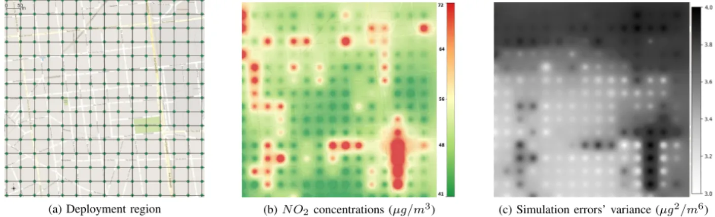
(a) Deployment region (b)N O2concentrations (µg/m3) (c) Simulation errors’ variance (µg2/m6)
Fig. 2: Deployment region, simulation of 2008 annual concentrations of N O2 and simulation errors corresponding to the
district of La-part-dieu, Lyon, France.
to interpolation-based deployment. After that, we evaluate the coverage results. Finally, we assess the impact of pollution estimation requirements on the network connectivity.
A. Dataset
In order to consider the real dispersion of air pollutants in the simulated pollution concentrations, we perform the evalua-tion of our proposal on monthly polluevalua-tion data corresponding to the 2008 Nitrogen Dioxide (N O2) concentrations in the
Lyon district of La-Part-Dieu, which is the heart of the Lyon City. To illustrate the pollution data set, we depict in Fig. 2b a pollution map that corresponds to the annual mean of 2008. This pollution data set has been generated by an enhanced atmospheric dispersion simulator called SIRANE [21], which is designed for urban areas and takes into account the impact of street canyons on pollution dispersion. The dataset has been provided by LMFA, which is a research lab specialized in fluid mechanics in the Lyon city, France.
The deployment region has a spatial resolution of 50 meters and is depicted in Fig. 2a. We consider as potential positions of nodes all the grid points (225 in total). We calculate the correlation coefficients Wpq using an exponential decay
function. That is, the correlation between points decrease exponentially with the euclidean distance.
We recall that the main input of our deployment approach is the variance of the errors of the physical model. In this evaluation part, we assume that the errors of the model are linearly correlated with its concentrations. Let γ express the linear relationship between the model concentrations and the model errors. Thus, we first calculate the variance of the concentrations of the physical model based on the 12 monthly pollution maps and then we multiply these variances by γ2
to get the variance of the physical model errors. We calculate the γ parameter by evaluating the linear regression between the concentrations of the dataset of the physical model and the real data of the few monitoring stations which are already deployed in the Lyon city. The resulting variance map of the physical model errors is depicted in Fig. 2c. Default simulation parameters are summarized in TABLE II. We fix the maximum
number of sinks to1 in order to get mono-sink networks since the deployment region is relatively small.
Parameter Notation Value
Number of discrete points (deployment region) N 225 Communication range of sensor nodes R 100m
The maximum number of sinks I 1
The cost of deploying a sensor at pointp δp 1
The cost of deploying a sink at pointp ψp 10
TABLE II: Default values of main simulation parameters.
B. Proof-of-concept
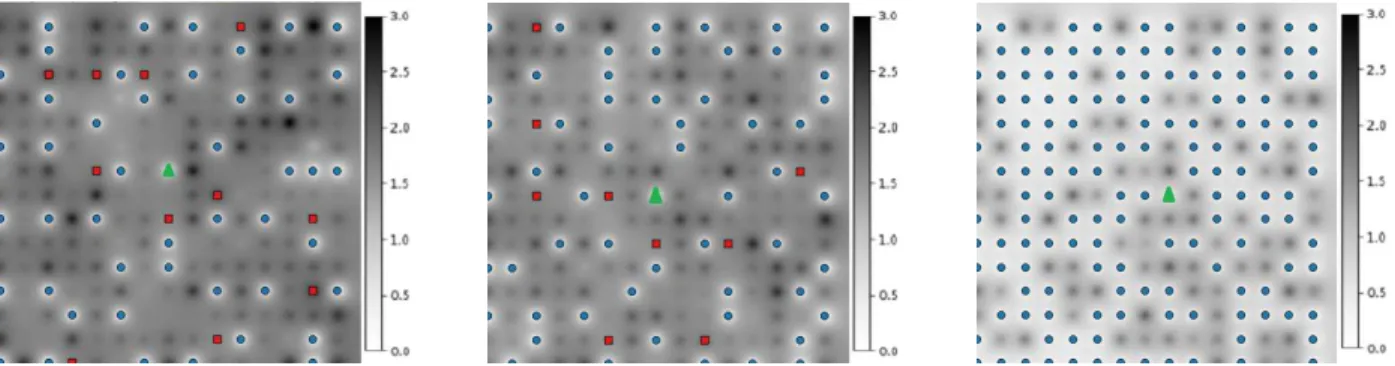
In order to provide a proof of concept of our assimilation-based coverage formulation, we consider 3 different values for the deployment budget and evaluate the assimilation error provided by the sensor network that is generated by our model. We first consider only the coverage constraints to get the positions of sensor nodes and then we add the connectivity constraints to obtain the positions of the sink and relay nodes which are used only for connectivity. We depict in Fig. 3 the positions of sensors, relay nodes and sinks for the three simulation cases. Sensors are placed near streets because these are heavily polluted areas and therefore have the most of uncertainty in physical models.
We also evaluate at each point of the map the corresponding assimilation error. We notice that the assimilation error is reduced when providing higher deployment budget. This is expected since better deployment precision requires more sensor nodes. In addition, Fig. 3 shows that the obtained nodes form a connected network as formulated in our connectivity constraint.
C. Comparison to interpolation-based deployment
In this simulation case, we compare our optimization model to the most related work where authors propose a deployment model allowing to minimize the estimation error of pollution concentration based only on sensor measurements [3]. In the work of Boubrima et al. [3], authors optimize the deployment by considering the model as a reference without taking into
Fig. 3: Proof-of-concept: optimal WSN topology and the corresponding estimation errors’ variance (µg2/m6
) while considering different values of the deployment budget (from left to right: respectively 68, 75 and 155 monetary units). Sensors (respectively relay nodes and sinks) are depicted in blue circles (respectively red squares and green triangles). Note that the scale in these 3 figures is different than the scale of Fig. 2c.
accounts the model errors. Their estimation of pollution is based only on the measurements of sensors in contrary to our work where both the physical model and the measurements are used in the estimation process.
In order to compare our work to [3], we vary the deployment budget and then execute our model based on the variance of the errors and the correlation between the points. We then execute the model of [3] by taking the physical model concentrations as a reference. Once we get the deployment result for each approach, we evaluate the estimation error by running 100 simulations, in each simulation the model errors are considered Gaussian. We then calculate based on these 100 simulations the estimation error’ variance maps. Finally, we plot the average of the estimation error variance over all the points for each value of the deployment budget in Fig. 4. Results show that the assimilation approach gives better estimation compared to the interpolation approach. This is mainly due to minimizing the variance of the estimation errors in the optimization process rather than trying to get interpolation results that resemble the model as in the work of [3]. Moreover, the difference between the two approaches decreases as the deployment budget increases since the esti-mation is less used when more sensors are available.
Fig. 4: Comparison results.
D. Evaluation of the coverage results
We now evaluate the optimal coverage results of our de-ployment model while analyzing the impact of sensing errors.
Results are depicted in Fig. 5 where the overall deployment cost is evaluated in function of both the assimilation error and the sensing error of sensors. We notice that the maximum improvement of the assimilation depends on the quality of sensors. Indeed, when sensors are not perfect, the least assim-ilation error that we can get is equal to 1µg2
/m6
. We also notice that a minimum number of sensors is required in order to be able to use the assimilation technique. This minimum number is equal to 50 sensors in our simulations. This means that in order to reduce the error of the physical model, we need 50 sensors or more. Finally, Fig. 5 shows that the more the tolerated assimilation error, the less the impact of the quality of sensors.
Fig. 5: Coverage results.
E. Evaluation of the connectivity results
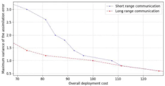
Finally, we evaluate the impact of the connectivity technol-ogy on the use of the deployment budget and the quality of data assimilation. We consider two different types of nodes depending on their communication capabilities: nodes with a communication range equal to 100m that we consider as short range communication nodes (like 802.15.4 for instance); and nodes with a communication range equal to 500m that we consider as long-range communication nodes (like LoRa for instance). We vary the deployment budget and depict the resulting assimilation error in Fig. 6. Results show that using long range communications leads to less assimilation
error when compared to short range communications with respect to the same value of the deployment budget. This is explained by the relay nodes added just to ensure connectivity in the case of short range communications, which means that the deployment optimization of some nodes is performed to improve connectivity but not necessarily coverage. Fig. 6 also shows that when the deployment budget increases, the difference between the two communication technologies decreases because the deployment of coverage nodes becomes so dense that the network is usually already connected even when using short range communications.
Fig. 6: Impact of the communication technology.
VII. CONCLUSION AND FUTURE WORK
In this paper, we tackle the deployment issue of sensor networks and propose a mixed integer programming model and a heuristic algorithm allowing to ensure an effective data assimilation of air pollution measurements in order to correct physical model simulations. Our main contribution is to define an appropriate coverage formulation for pollution data assimilation and then derive a deployment approach using integer linear programming and linear relaxation. We applied our approach on a dataset of the Lyon City, France and showed that the assimilation-based deployment outperforms the interpolation-based one. We have also assessed by sim-ulation the impact of the input parameters of our approach, mainly the quality of sensors and their communication range, on the deployment results. As a perspective, we plan to evaluate our approach using other datasets with different urban characteristics.
ACKNOWLEDGMENT
This work has been supported by the "LABEX IMU" (ANR-10-LABX-0088) of Université de Lyon, within the program "Investissements d’Avenir" (ANR-11-IDEX-0007) operated by the French National Research Agency (ANR).
REFERENCES
[1] Z. Li, N. Wang, A. Franzen, P. Taher, C. Godsey, H. Zhang, and X. Li, “Practical deployment of an in-field soil property wireless sensor network,” Computer Standards & Interfaces, vol. 36, no. 2, pp. 278–287, 2014.
[2] A. Marjovi, A. Arfire, and A. Martinoli, “High resolution air pollu-tion maps in urban environments using mobile sensor networks,” in
Distributed Computing in Sensor Systems (DCOSS), 2015 International Conference on. IEEE, 2015, pp. 11–20.
[3] A. Boubrima, W. Bechkit, and H. Rivano, “Error-bounded air quality mapping using wireless sensor networks,” in Local Computer Networks
(LCN), 2016 IEEE 41st Conference on. IEEE, 2016, pp. 380–388. [4] C. Zhu, C. Zheng, L. Shu, and G. Han, “A survey on coverage and
connectivity issues in wireless sensor networks,” Journal of Network
and Computer Applications, vol. 35, no. 2, pp. 619–632, 2012. [5] B. Liu, O. Dousse, P. Nain, and D. Towsley, “Dynamic coverage
of mobile sensor networks,” Parallel and Distributed Systems, IEEE
Transactions on, vol. 24, no. 2, pp. 301–311, 2013.
[6] K. Chakrabarty, S. S. Iyengar, H. Qi, and E. Cho, “Grid coverage for surveillance and target location in distributed sensor networks,”
Computers, IEEE Transactions on, vol. 51, no. 12, pp. 1448–1453, 2002. [7] ˙I. K. Altınel, N. Aras, E. Güney, and C. Ersoy, “Binary integer programming formulation and heuristics for differentiated coverage in heterogeneous sensor networks,” Computer Networks, vol. 52, no. 12, pp. 2419–2431, 2008.
[8] X. Chang, R. Tan, G. Xing, Z. Yuan, C. Lu, Y. Chen, and Y. Yang, “Sensor placement algorithms for fusion-based surveillance networks,”
IEEE Transactions on Parallel and Distributed Systems, vol. 22, no. 8, pp. 1407–1414, 2011.
[9] M. E. Keskin, ˙I. K. Altınel, N. Aras, and C. Ersoy, “Wireless sensor network lifetime maximization by optimal sensor deployment, activity scheduling, data routing and sink mobility,” Ad Hoc Networks, vol. 17, pp. 18–36, 2014.
[10] M. Rebai, H. Snoussi, F. Hnaien, L. Khoukhi et al., “Sensor deployment optimization methods to achieve both coverage and connectivity in wireless sensor networks,” Computers & Operations Research, vol. 59, pp. 11–21, 2015.
[11] S. Sengupta, S. Das, M. Nasir, and B. K. Panigrahi, “Multi-objective node deployment in wsns: In search of an optimal trade-off among coverage, lifetime, energy consumption, and connectivity,” Engineering
Applications of Artificial Intelligence, vol. 26, no. 1, pp. 405–416, 2013. [12] J. Ranieri, A. Chebira, and M. Vetterli, “Near-optimal sensor placement for linear inverse problems,” IEEE Transactions on signal processing, vol. 62, no. 5, pp. 1135–1146, 2014.
[13] V. Roy, A. Simonetto, and G. Leus, “Spatio-temporal sensor manage-ment for environmanage-mental field estimation,” Signal Processing, vol. 128, pp. 369–381, 2016.
[14] P. G. Liaskovitis and C. Schurgers, “Leveraging redundancy in sampling-interpolation applications for sensor networks: A spectral approach,”
ACM Transactions on Sensor Networks (TOSN), vol. 7, no. 2, p. 12, 2010.
[15] A. Krause, A. Singh, and C. Guestrin, “Near-optimal sensor placements in gaussian processes: Theory, efficient algorithms and empirical stud-ies,” Journal of Machine Learning Research, vol. 9, no. Feb, pp. 235– 284, 2008.
[16] A. Krause, C. Guestrin, A. Gupta, and J. Kleinberg, “Robust sensor placements at informative and communication-efficient locations,” ACM
Transactions on Sensor Networks (TOSN), vol. 7, no. 4, p. 31, 2011. [17] W. Du, Z. Xing, M. Li, B. He, L. H. C. Chua, and H. Miao, “Sensor
placement and measurement of wind for water quality studies in urban reservoirs,” ACM Transactions on Sensor Networks (TOSN), vol. 11, no. 3, p. 41, 2015.
[18] A. Boubrima, W. Bechkit, and H. Rivano, “Optimal wsn deployment models for air pollution monitoring,” IEEE Transactions on Wireless
Communications, vol. 16, no. 5, pp. 2723–2735, 2017.
[19] ——, “A new wsn deployment approach for air pollution monitoring,” in Consumer Communications & Networking Conference (CCNC), 2017
14th IEEE Annual. IEEE, 2017, pp. 455–460.
[20] V. Gallart, S. Felici-Castell, M. Delamo, A. Foster, and J. J. Perez, “Evaluation of a real, low cost, urban wsn deployment for accurate en-vironmental monitoring,” in Mobile Adhoc and Sensor Systems (MASS),
2011 IEEE 8th International Conference on. IEEE, 2011, pp. 634–639. [21] L. Soulhac, P. Salizzoni, P. Mejean, D. Didier, and I. Rios, “The model sirane for atmospheric urban pollutant dispersion; part II, validation of the model on a real case study,” Atmospheric Environment, vol. 49, pp. 320–337, 2012.
[22] M. Asch, M. Bocquet, and M. Nodet, Data assimilation: methods,
algorithms, and applications. SIAM, 2016.
[23] W. Revelle, “An introduction to psychometric theory with applications in r,” 2009.