Classification of vocal fold vibration as regular or irregular in normal, voiced speech

Classification of vocal fold vibration as regular or

irregular in normal, voiced speech

by

Kushan Krishna Surana

Submitted to the Department of Electrical Engineering and Computer

Science

in partial fulfillment of the requirements for the degree of

Master of Engineering in Computer Science and Engineering

at the

MASSACHUSETTS INSTITUTE OF TECHNOLOGY

February 2006

©

Massachusetts Institute of Technology 2006. All rights reserved.

A u th o r ...

Department of Electrical Engineering and Computer Science

February 3, 2006

Certified by...

Janet Slifka

Research Scientist

Thesis Supervisor

Accepted by ...

Arthur C. Smith

Chairman, Department Committee on Graduate Students

MASSACHUSETTg IN&IITIU I E OF TECHNOLOGY

AUG

₁₄

2006

Classification of vocal fold vibration as regular or irregular in

normal, voiced speech

by

Kushan Krishna Surana

Submitted to the Department of Electrical Engineering and Computer Science on February 3, 2006, in partial fulfillment of the

requirements for the degree of

Master of Engineering in Computer Science and Engineering

Abstract

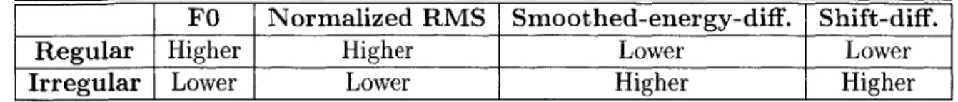
Irregular phonation serves an important communicative function in human speech and occurs allophonically in American English. This thesis uses cues from both the temporal and frequency domains - such as fundamental frequency, normalized RMS amplitude, smoothed-energy-difference amplitude (a measure of abruptness in energy variations) and shift-difference amplitude (a measures of periodicity) - to classify segments of regular and irregular phonation in normal, continuous speech.

Support Vector Machines (SVMs) are used to classify the tokens as examples of either regular or irregular phonation. The tokens are extracted from the TIMIT database, and are extracted from 151 different speakers. Both genders are well repre-sented, and the tokens occur in various contexts within the utterance. The train-set uses 114 different speakers, while the test-set uses another 37 speakers. A total of 292 of 320 irregular tokens (recognition rate of 91.25% with a false alarm rate of 4.98%), and 4105 of 4320 regular tokens (recognition rate of 95.02% with a false alarm rate of

8.75%) are correctly identified. The high recognition rates are an indicator that the

set of acoustic cues are robust in accurately identifying a token as regular or irregular, even in cases where one or two acoustic cues show unexpected values.

Also, analysis of irregular tokens in the training set (1331 irregular tokens) shows that 78% occur at word boundaries and 5% occur at syllable boundaries. Of the irreg-ular tokens at syllable boundaries, 72% are either at the junction of a compound-word

(e.g "outcast") or at the junction of a base word and a suffix. Of the irregular tokens which do not occur at word or syllable boundaries, 70% occur adjacent to voiceless consonants mostly in utterance-final location. These observations support irregular phonation as a cue for syntactic boundaries in connected speech, and combined with the robust classification results to separate regular phonation from irregular phona-tion, could be used to improve speech recognition and lexical access models.

Thesis Supervisor: Janet Slifka Title: Research Scientist

Acknowledgments

This thesis was supported by NIH

#

I would like to thank my advisor, Dr. Janet Slifka for her guidance and support.

I've had the pleasure of working with her as a UROP and a graduate student, and have found it to be an invaluable experience.

I would also like to thank the Speech Group, specifically Professor Kenneth Stevens, Joseph Perkell, Stefanie Shattuck-Hufnagel, Helen Hanson, Sartrajit Ghosh, Seth Hall, Arlene Wint, Lan Chen, Yoko Saikachi, Tomas Bohm and Steven Lulich for their support. The Speech Group is truly a fantastic place to work and I will always cherish the time I spent there.

I've been fortunate to have had contact with some amazing people at MIT. There are far too many mention, but I would like to express my thanks to Professors George Verghese and Ronald Parker.

Finally, I would like to thank my family. To my parents for their love, and my brothers Kanishka and Kunal for their unconditional support.

Contents

1 Introduction 13

1.1 Irregular phonation . . . . 13

1.2 Types of irregular phonation . . . . 16

1.3 Specific A im . . . . 19

2 Motivation 21 2.1 Lexical Access From Features (LAFF) Project . . . . 21

2.1.1 T heory . . . . 21

2.1.2 Relevance of irregular phonation . . . . 24

2.2 Applicability beyond LAFF Project . . . . 25

3 Prior Work 27 3.1 Kiessling, Kompe, Niemann, N6th & Batliner, 1995 . . . . 27

3.2 Ishi, 2004 . . . . 29 3.3 Comments . . . . 31 4 Speech corpora 33 4.1 Choice of Database . . . . 33 4.2 Database characteristics . . . . 34 5 Method 37 5.1 Cue selection . . . . 37

5.1.1 Fundamental Frequency (FO) . . . . 38

5.1.3 Smoothed-energy-difference amplitude . . . . 42

5.1.4 _{Shift-difference amplitude . . . .} 46

6 Analysis 53 6.1 Overview . . . . 53

6.2 Distribution pattern . . . . 54

6.3 Failure analysis for each cue . . . . 56

6.3.1 Fundamental Frequency (FO) . . . . 56

6.3.2 Normalized RMS amplitude . . . . 60

6.3.3 Smoothed-energy-difference amplitude . . . . 62

6.3.4 Shift-difference amplitude . . . . 65

6.3.5 Summary . . . . 67

6.4 Failure analysis for all cues . . . . 70

7 Classification 73 7.1 Support Vector Machines . . . . 73

7.1.1 Theory . . . . 73

7.1.2 RBF (Gaussian) kernel . . . . 74

7.1.3 Results . . . . 74

8 Irregular phonation as a segmentation cue 79 8.1 Introduction . . . . 79

8.2 Data set . . . . 80

8.3 Results . . . . 81

8.4 Discussion . . . . 87

List of Figures

1-1 Examples of irregular phonation . . . . 18

4-1 Duration of regular and irregular tokens . . . . 35

5-1 Illustration of FO computation for a regular and an irregular token . . 41

5-2 Illustration of RMS computation for a regular and an irregular token 43

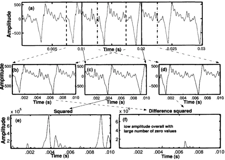
5-3 Illustration of smoothed-energy-difference amplitude calculation for a

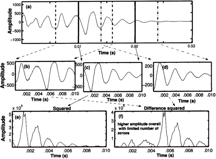
regular token . . . . 47 5-4 Illustration of smoothed-energy-difference calculation for an irregular

token... ... 48

5-5 Illustration of shift-difference amplitude calculation for a regular token 51 5-6 Illustration of shift-difference amplitude calculation for an irregular token 52 6-1 Distribution of the acoustic cues for regular and irregular tokens. . . . 55

6-2 Illustration of misleading FO estimates for irregular phonation . . . . 58

6-3 Illustration of misleading FO estimates for regular phonation . . . . . 59

6-4 Examples of vocal fry with FO estimates as high as 100 Hz for two different female speakers. (Source of waveform: TIMIT,1990) . . . . . 61 6-5 Illustration of misleading normalized RMS estimates for regular and

irregular phonation . . . . 63 6-6 Illustration of misleading smoothed-energy-difference estimates for

ir-regular phonation . . . . 64

6-7 Illustration of misleading smoothed-energy-difference estimate for

6-8 Illustration of misleading shift-difference estimates for irregular

phona-tio n . . . . 68 6-9 Two examples of regular tokens with misleading shift-difference estimates 69 6-10 Examples of regular and irregular tokens with misleading estimates for

all four acoustic cues . . . . 71 7-1 ROC curves for the classification of irregular tokens . . . . 77

8-1 Breakdown of irregular phonation at word and syllable boundaries.

The absolute number is shown next to the percentage within brackets. (Based on 1331 tokens) . . . . 82 8-2 Breakdown of irregular phonation at syntactic phrase and utterance

boundaries. The absolute number is shown next to the percentage within brackets. (Based on 1331 tokens) . . . . 83 8-3 Breakdown of irregular phonation at voiceless stops and vowel-vowel

boundaries, The absolute number is shown next to the percentage within brackets. (Based on 1331 tokens) . . . . 83

8-4 Breakdown of irregular phonation at word level boundaries for vowel-vowel junctions and voiceless stops. . . . . 84

8-5 Breakdown of irregular phonation which does not occur at word or syllable boundaries. . . . . 86 8-6 Two examples of irregular phonation which do not occur at word

boundaries. (a) is an example of an irregular token adjacent to a voice-less consonant in utterance-final location while (b) shows an irregular token in vowel-medial position. . . . . 86

List of Tables

2.1 List of distinctive features for American English grouped by articulator-free and articulator-bound classes (Slifka et. al, 2004) . . . . 23

2.2 List of distinctive features for the words "debate", "wagon" and "help" (Stevens, 2002) . . . . 23 3.1 Expected values of the cues for regular and double periodic irregular

phonation (Ishi, 2004) . . . . 31 3.2 Expected values of the cues for low fundamental frequency irregular

phonation (Ishi, 2004) . . . . 31

4.1 List of vowels used to denote regular phonation . . . . 35

4.2 Number of regular and irregular tokens based on duration of tokens . 36 5.1 Expected behavior of an ideal FO estimator to distinguish between

regular and irregular phonation. . . . . 38 5.2 Number of FO estimates below 72 Hz for regular and irregular tokens

using different threshold values . . . . 40

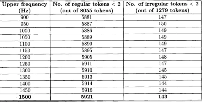
5.3 Number of smoothed-energy-difference estimates below 2 for regular and irregular tokens using different cutoffs for the higher frequency band 45 5.4 Number of smoothed-energy-difference estimates below 2 for regular

and irregular tokens using different lower smoothing window sizes for averaging the energy . . . . 46

6.1 Two-sample t-test on the four acoustic cues with the null hypothesis that the means are equal (df 9332). . . . . 54

6.2 Common causes of failure for each cue for regular and irregular tokens. 68 7.1 Area under ROC curve using 959 irregular tokens and different number

of regular tokens for training the SVM. The same test-set, consisting of 4320 regular tokens and 320 irregular tokens, is used in all the cases. 76

8.1 Syntactic boundary labels for irregular token occurrence. . . . . 81 8.2 Contexts in which irregular phonation at word-medial position occur

Chapter 1

Introduction

Currently, robust systems to classify and detect irregular phonation do not exist. This thesis aims to address this issue and builds upon existing studies of irregular phonation. In this chapter, irregular phonation is defined and described in terms of its segmental and acoustic correlates in the speech waveform. Some common types of irregular phonation are also described and the specific aim of this thesis is detailed.

1.1

Irregular phonation

The source-filter model of speech production, as set up by Fant (1960), proposes that human speech is a consequence of the generation of one or more sources of sound and the filtering of these sounds by the vocal tract. One type of sound source results from the vibration of the vocal folds and is the result of a delicate balance of the subglottal air pressure that drives the folds apart, and the muscular, elastic and Bernoulli forces that bring them together. Sounds produced in this manner are generally referred to as voiced sounds.

Normal, voiced speech, or regular phonation, is characterized by the quasi-regular vibration of the vocal folds. Although the vocal folds will oscillate quasi-regularly in general when the variables transglottal pressure, vocal fold tension, and vocal fold adduction - among others - are in particular ranges, irregularities in the vocal fold vibrations are observed for certain combinations of the values of these variables.

These irregularities in vocal fold vibration lead to the observation of irregularities in the speech waveform, and are more pronounced than the small-scale cycle-to-cycle variations observed in quasi-periodic, normal, voiced speech.

The small-scale variations during normal, voiced speech mentioned above have been enumerated and defined by Titze (1995, p. 338-340):

" jitter: "a short-term (cycle-to-cycle) variation in the fundamental frequency of

a signal."

" shimmer: "a short-term (cycle-to-cycle) variation in the amplitude of a signal." " perturbation: "a disturbance, or small change, in a cyclic variable (period,

amplitude, open quotient, etc.) that is constant in regular periodic oscillation."

" tremor: "a 1-15 Hz modulation of a cyclic parameter (e.g., amplitude or

fun-damental frequency), either of a neurologic origin or an interaction between neurological and biomechanical properties of the vocal folds."

Papers dealing with the subject of voice quality and phonation often use the terms "modal" and "periodic" interchangeably with regular phonation. Similarly, "nonmodal" and "aperiodic" are often used to denote irregular phonation. This thesis avoids the use of these terms as they are not synonymnous with regular or irregular phonation. For example, nonmodal phonation includes irregular, aperiodic phonation such as vocal fry as well as regular, periodic phonation such as breathy voice. Regions in the speech waveform with very low frequency, periodic glottal pulses are also not typical of the quasi-periodic pulses in the phonation for a given speaker at a given time with the auditory impression of a "...rapid series of taps, rather like the sound of a stick being run along a railing." (Catford, 1977, p.98). These regions are classified as irregular in this thesis, in spite of being periodic.

Based on an initial survey of the literature and the specific aims of the system, a specific definition for irregular phonation was formulated to contrast it with regular phonation and its small-scale variations:

"A region of speech is an example of irregular phonation if the speech waveform displays either an unusual difference in time or amplitude over adjacent pitch periods that exceeds the small-scale jitter and shimmer differences or an unusually wide-spacing of the glottal pulses compared to their spacing in the local envi-ronment, indicating an anomaly from the usual, quasi-periodic behavior of the vocal folds."

Irregular phonation occurs in a number of contexts in American English, ranging from a single glottal closure accompanying a consonantal segment to a change in voice source characteristics over a region encompassing several segments or even syllables. Irregular phonation also commonly occurs allophonically in certain contexts. For ex-ample, in American English, vowel initial words may be produced irregularly at onset (e.g "elephant") (Dilley & Shattuck-Hufnagel, 1995); in syllable-final environments, voiceless stop consonants, particularly /t/, may be realized as a glottal stop (e.g. in "hat rack") (Pierrehumbert, 1995); and allophonic irregular phonation may often be associated with vowels adjacent to a glottal stop, with languages differing in the duration of this allophonic irregularity (Blankenship, 2002).

The study of irregular phonation is also relevant for languages other than Amer-ican English. Gordon and Ladefoged (2001) completed a survey which shows how languages use irregular phonation contrastively to distinguish among word forms. Hausa and certain other Chadic languages use irregular phonation contrastively for stops. Some other Northwest American Indian languages, e.g., Kwakwila, Montana Salish, Hupa, and Kashaya Pom, contrast irregular and regular voicing among their sonorants. Laver (1980) and others have also suggested that certain languages use irregular phonation to signal a speaker's turn. For example, irregular phonation may mark the end of a turn in London Jamaican (Local, Wells & Sebba, 1985).

In acoustic terms, irregular phonation is generally associated with irregularly spaced pitch periods and is often accompanied by other characteristics, such as full damping, low FO, breathiness or low amplitude (Ladefoged, 1971; Fischer-Jorgenson,

believed to contribute to the perceptual impression of a glottal gesture or disturbance in the regular voice quality (Rozyspal & Millar, 1979; Hillenbrand & Houde, 1996; Pierrehumbert & Frisch, 1997).

Various theories and studies have tried to explain the physiological basis for irreg-ular phonation. One theory suggests that from the perspective of vocal fold dynamics, regular and irregular phonation may be distinguished based on the entrainment or lack of entrainment of natural vibratory modes of the vocal folds, called eigenmodes (Berry, 2001). Slifka (2000) conducted a study which suggests that as the glottal configuration moves from one setting to another, it could move through regions of in-stability leading to irregular phonation. Hanson, Stevens, Kuo, Chen & Slifka (2001) have tried to explain the physiological variations during irregular phonation by ex-ploring how the glottal waveform and vocal tract transfer function are affected by the various patterns of complete/incomplete/nonsimultaneous closing of the vocal folds during phonation. These studies contrast the incomplete closing of the vocal folds in irregular phonation to regular phonation which has been defined as phona-tion in which full contact occurs between the vocal folds during the closed phase of a phonatory cycle (Titze, 1995).

1.2

Types of irregular phonation

The articulatory mechanism may affect the kinds of irregular vocal fold vibrations produced. Over the years, researchers have classified irregular phonation into sub-groups based on a combination of physiological, perceptual and acoustic character-istics. Various terms have been used interchangeably to describe these sub-groups with papers dedicated to establishing a taxonomy of irregular phonation (Gerrat & Kreiman, 2001). This section describes some of of these terms.

* Creaky phonation : "...typically associated with vocal folds that are tightly adducted but open enough along a portion of their lengths to allow for voicing" (Gordon & Ladefoged, 2001, p.386). This is often accompanied by irregularly spaced pitch periods and decreased acoustic intensity relative to regular

phona-tion (Gordon & Ladefoged, 2001, p.387). An example of creaky phonaphona-tion is shown in Figure 1-1 (a).

" Vocal fry : It is usually defined as a train of discrete, laryngeal excitations

of extremely low frequency, with almost complete damping of the vocal tract between excitations (Hollien, Moore, Wendahl & Michel, 1966) giving the au-ditory impression of a "...rapid series of taps, rather like the sound of a stick being run along a railing."(Catford, 1977, p.98). One of vocal fry's distinct characteristics is that the vocal folds tend to vibrate so slowly that individual vibrations can be perceived (Colton & Casper, 1996). Vocal fry is characterized

by a very short open period and a very long period where the vocal folds are

completely adducted (Blomgren, Chen, Ng & Gilbert, 1998, p.2650). Zemlin

(1988, p.166) reported that examination of vocal fry with high speed photogra-phy revealed that "...the folds are approximated tightly, but at the same time they appear flaccid along their free borders, and subglottal air simply bubbles up between them at about the junction of the anterior two-thirds of the glottis". An example of vocal fry is shown in Figure 1-1 (b).

" Glottalization : Titze (1995, p.338) has defined it as "...transient sounds resulting from the relatively forceful adduction or abduction of the vocal folds [with the perceptual impression of] a voice that contains frequent transition sounds (clicks)." Huber (1992) defines this term as an initial vibratory cycle clearly demarcated from the rest of the periodic glottal vibrations, which is in contrast to the more common reference of glottalization occurring at other locations in the speech signal, including in phrase final position. An example of glottalization is shown in Figure 1-1 (c).

" Diplophonia : "...simultaneous production by the voice of two separate tones" (Ward, Sanders, Goldman & Moore, 1969, p.771). Titze (1995, p.337) restricts the two tones to be dependent, the frequency of one tone an octave lower than the other, but this study assumes no such rational dependence. An example of diplophonia is shown in Figure 1-1 (d).

(a) Creaky voice 0.01 0.02 0.03 0.04 0.05 0.06 Time (s) 0.05 Time (s) 0.1

II

Figure 1-1: Some different types of irregular phonation: (a) Creaky voice (b) Vocal fry (c) Glottalization (d) Diplophonia. (Source of waveforms: TIMIT, 1990)

The examples above offer a glimpse into the range of variations in irregular phona-tion in normal speech. Some of the definiphona-tions offer concrete physiological character-istics associated with a particular type of irregular phonation, but a lot more remains to be understood regarding the physiological mechanism of irregular phonation pro-duction. Detailed models of vocal fold functions such as those developed by Titze & Talkin (1979) and studies done by Hanson et. al. (2001) and Slifka (2005) may help enhance our understanding about irregular phonation.

1000 1 500 CL ₀ E -500 -1000 UL, 200 0 0 -10 -2 E -10 -20 (c) Glottalization II. I, 0 -0. 0.06 0.08 I

1.3

Specific Aim

This thesis attempts to use signal-processing techniques, in either the temporal or frequency domain, to analyze the systematic variations in examples of irregular vocal fold vibration that distinguish them from examples of regular vocal fold vibration. Acoustically, this translates to proposing a set of acoustic cues capable of distinguish-ing between regions of periodic, glottal pulses and (1) regions of aperiodic pulses, (2) single aperiodic pulses or, (3) regions of atypically large spacing between adjacent glottal pulses (as compared to the glottal pulse spacing in the local environment).

Another aim of this thesis is to study the context for occurrences of irregular phonation. In other words, given an occurrence of irregular phonation, is there a specific context where it is more likely to occur than others? The following contexts are observed: (1) utterance-boundaries, (2) word-boundaries, (3) syllable-boundaries, (4) voiceless-stops /p/, /t/ and /k/ and (5) vowel-medial locations.

Chapter 2

Motivation

Irregular phonation in the form of regions of creakiness, period doubling, irregular pitch periods and amplitude modulation can occur in the speech of normal as well as pathological talkers (Docherty, 2001, p.364). This chapter details the benefits of an accurate classification system to distinguish between regular and irregular phonation.

2.1

Lexical Access From Features (LAFF) Project

The work done in this thesis falls under the purview of the Lexical Access From Features (LAFF) Project (Stevens, 2002), which proposes a model where words are represented in the mental lexicon as a sequence of segments, each of which is described

by a set of binary distinctive features. Although the results of this work are widely

applicable, this section of the thesis focuses exclusively on the role this thesis plays within the LAFF Project. In order to adequately describe this role, a brief overview

of the project is required.

2.1.1

Theory

The LAFF Project considers words to be represented as sequences of segments (also referred to as phonemes), each of which can be defined by a set of binary distinctive features (Jakobson, Fant, and Halle, 1952). These features specify the phonemic

contrasts that are used in a particular language so that a change in one feature leads to a different word. The project proposes the existence of a universal set of features, with every language defined by a unique subset drawn from these features. The end goal of the project is to decompose any utterance into a series of feature bundles, assign a probabilistic estimate to the features within a segment and arrive at a hypothesis for the underlying word sequence. In order to achieve this goal, the initial focus is on building a system which can correctly identify all the distinctive features for American English.

As a first step towards the goal of arriving at a feature set, the LAFF Project aims to identify "landmarks" for the acoustic waveform. Landmarks are regions in the acoustic waveform which either show a peak in frequency amplitude, a low-frequency minima or acoustic discontinuities. These landmarks are detected based on amplitude changes in various energy bands (Stevens, 2002; Lin 1995; Slifka, Stevens, Manuel, Shattuck-Hufnagel, 2004).

The type of landmark region provides evidence for a broad class of distinctive features called "articulator-free" features. These features refer to the general char-acteristic of the constrictions within the vocal tract and the acoustic consequences of these constrictions. There is another class of features called "articulator-bound" features which are derived from the acoustic cues sampled near the landmark region.

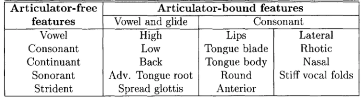
The articulator-bound features provide information about the action of the particu-lar articulator used in producing the phoneme. Table 2.1 (Slifka et. al, 2004) shows a list of distinctive features for American English grouped by articulator-free and articulator-bound classes.

Each phoneme is characterized by a unique combination of these articulator-free and articulator-bound features. The feature set is arranged in a heirarchical structure, which implies that the entire feature set does not need to be specified since some features can be inferred from others. Table 2.2 (Stevens, 2002) shows the lexical representations of the words "debate", "wagon" and "help" to illustrate this point.

Each distinctive feature is considered to have a defining articulatory action and a correspoding acoustic correlate. An example is the feature [back] for vowels. For

Table 2.1: List of distinctive features for American English grouped by articulator-free and articulator-bound classes (Slifka et. al, 2004)

Articulator-free Articulator-bound features features Vowel and glide Consonant

Vowel High Lips Lateral

Consonant Low Tongue blade Rhotic

Continuant Back Tongue body Nasal

Sonorant Adv. Tongue root Round Stiff vocal folds

Strident Spread glottis Anterior I _I

Table 2.2: List of distinctive features for the words "debate", "wagon" and "help" (Stevens, 2002)

debate wagon help

d 9 b e t w a g 9 n h e I p vowel + + + + + glide

+

+

+

+

+

+

-adv. tongue root +

+

-spread glottis +

nasal

+

[+back] vowels, the tongue body is displaced back to form a narrowing in the pharyn-geal or posterior oral cavity. The acoustic consequence is a second-formant frequency that is low and close to the first-formant frequency. Vowels classified as [-back], on the other hand, are produced with the tongue body forward and a high second-formant frequency (Stevens, 2002).

It is clear that based on the model proposed by the LAFF Project, landmark detection is inarguably the first and most important step in finding the underlying word sequence of an utterance.

2.1.2

Relevance of irregular phonation

In addition to landmarks, there are other regions in the utterance which might show characteristics similar to those observed for landmarks (i.e. peaks, valleys or disconti-nuities in certain frequency ranges). Some of these regions are classified as "acoustic events". Irregular phonation is one example of such an acoustic event. The presence of irregular phonation can hence result in incorrect landmark indentification. Due to the frequent occurrence of irregular phonation in normal speech, detecting this par-ticular acoustic event and distinguishing it from landmarks is especially important. To cite one example where irregular phonation is responsible for incorrect landmark identification, regions of irregular phonation are often classified as vowel landmarks

by the landmark identifier. If the regions of irregular phonation are correctly

identi-fied, the misclassification of landmarks could be greatly reduced, which would result in more accurate articulator-free feature identification and also lay a more robust framework for articular-bound feature identification.

The identification of irregular phonation could also help in the detection of ut-terance and word boundaries and lay the groundwork for estimating the prosodic structure of an utterance (see Chapter 8 for further discussion) - both of which are relevant to the LAFF Project.

2.2

Applicability beyond LAFF Project

Huber (1992, p.503) has conducted experiments to show that human listeners use ir-regularity in speech signals for segmentation purposes. These results are collaborated

by Blomgren, Chen, Ng & Gilbert (1998) who also observed that listeners were

con-sistently able to perceive glottal fry. Huber's research (1992), with that of Kreiman

(1982), show that irregular phonation is an important demarcation cue in connected

speech, used to support the segmentation of the continuous speech utterance into relevant information units in American English. Their research suggests that a bet-ter understanding of irregular phonation is essential to develop accurate and robust automatic speech recognition systems and human-like speech synthesis systems.

Irregular vocal phenomenon is also used to convey linguistic and nonlinguistic information. Gordon & Ladefoged (2001, p.383) note that a difference in phonation type might indicate a contrast between otherwise identical lexical items and bound-aries of prosodic constituents in many languages. Their statement is substantiated

by research done by Dilley, Shattuck-Hufnagel & Ostendorf (1996), Pierrehumbert & Talkin (1992) and Pierrehumbert (1995) who state that irregular phonation could

be exploited as a cue for recognizing prosodic patterns. This could improve auto-matic detection of prosodic markers, both for corpus transcription and for speech understanding applications (Dilley, Shattuck-Hufnagel & Ostendorf, 1996, p.438).

The detection of irregular phonation is also of interest for pathological speech. There are numerous medical conditions that affect voice quality. Many such condi-tions have their origins in the vocal system and the tools available for the detection of these speech pathologies are invasive or require expert analysis. Hence, a reliable, accurate and non-invasive automatic system for recognizing and monitoring speech abnormalities is one of the necessary tools in pathological speech assessment (Dibazar, Narayanan & Berger, 2002).

Since irregular phonation often interrrupts the periodicity of the speech segment, a key understanding of it will also aid in developing better FO estimation algorithms.

incorrect FO estimates for those regions could be avoided.

The relatively frequent occurence of irregular phonation in normal speech across languages, combined with its usefulness in terms of the acoustic cues it provides, makes its comprehensive study essential towards establishing a complete model of speech production and in developing robust algorithms for pitch detection, speech-synthesis and automatic speech recognition.

Chapter 3

Prior Work

There exists a wide range in the rate of occurrence of irregular phonation across individual speakers (Huber, 1988; Dilley et. al., 1996; Dilley & Shattuck-Hufnagel,

1995). Irregular phonation also occurs more often at certain locations in an utterance

over others. For example, Redi & Shattuck-Hufnagel (2001) found a higher rate of irregular phonation on words at the ends of utterances than on words at the ends of utterance-medial intonational phrases. In spite of the speaker-to-speaker and the context-to-context variations of irregular phonation, an ideal classification system trained to distinguish between regular and irregular phonation should be speaker-independent and context-speaker-independent.

There have not been many automatic classification systems proposed to classify regular and irregular phonation. To the author's knowledge, only Ishi (2004) and Kiessling, Kompe, Niemann, N6th & Batliner (1995) have addressed this topic ex-plicitly.

3.1

_{Kiessling, Kompe, Niemann, N*th & Batliner,}

1995

Kiessling et. al, 1995 proposes a recognition scheme for classifying frames of irregular phonation (referred to as "laryngealization" in the paper) from regular phonation

using two approaches; the first based in the frequency domain, and the second in the temporal domain. The database used in the study contained 1329 sentences from 4 speakers (3 female, 1 male) for a total of 30 minutes of speech. Frames of irregularity were labeled by two trained phoneticians resulting in 1191 frames.

The first approach in this study used cues from the spectrum, the cepstrally smoothed spectrum and the cepstrum of the speech waveform to disinguish between regular and irregular phonation. These cues were extracted based on the observation that the spectra and cepstra of irregular phonation differ from regular phonation (for example, a lack of a regular harmonic structure was observed in the cepstrally smoothed spectrum of irregular segments as compared to regular segments). Based on these differences, the following five cues were proposed:

- the sum of the vertical distances of neighboring extrema in the cepstrally smoothed spectrum below 1700 Hz.

- the average vertical distance of neighboring extrema in the cepstrally smoothed spectrum below 1700 Hz.

- the location of the absolute maximum in the cepstrum.

- the height of the absolute maximum in the cepstrum.

- the quotient of the largest and the second largest maximum in the cepstrum of the center-clipped signal (to eliminate the influence of the vocal tract).

These five cues were combined with normal mel-cepstral coefficients to train a phone component recognition system. The system was originally set to distinguish between 40 different phones using 11 mel-cepstral coefficients per frame and a Gaus-sian classifier, automatically clustering into 5 clusters per phone and a full covariance matrix. For all the phones which had more than 100 frames labeled as irregular in the database, a new additional phone label was introduced increasing the number of phones from 40 to 51. The 40 regular phones were mapped into one class and the remaining 11 irregular phones into another. The first portion of the experiment was

speaker-dependent for multiple speakers and yielded a recognition rate of 80% with a false alarm rate of 8% for irregular phonation. The second portion of the experiment used three speakers for training and one for testing to obtain a recognition rate of

67% with a false alarm rate of 7% for irregular phonation.

The second approach in this study used time domain cues. The approach proposed an inverse filtering technique using artificial neural networks. The output of the neural network was classified into three classes: unvoiced, regular voiced and irregular voiced. The sample values of the neural-network filter output were used as input for another artificial neural network trained to discriminate between the three classes. This approach resulted in a 65% recognition rate with a false alarm rate of 12% for irregular phonation. The paper does not mention if these results are speaker-dependent or speaker-inspeaker-dependent.

3.2

Ishi, 2004

Ishi, 2004 attempts to classify irregular phonation, referred to as "creaky voice", from regular and aspirated segments of speech using the ratio of the first two peaks of the autocorrelation function of the glottal excitation waveform as a primary cue.

In the study, the speech signal was first high-pass filtered at 60 Hz in order to prevent the waveform from gradually rising or falling. A 1st-order LPC-analysis was applied to the speech waveform. The estimated coefficient is referred to as the adap-tive emphasis coefficient (APE) in the study. The speech signal was then pre-emphasized using the APE, and subsequently 18th-order LPC-analysis was applied on the pre-emphasized signal. The obtained LPC coefficients were used for inverse filtering of the high-pass filtered speech signal. The residual signal was treated as the glottal excitation waveform.

The glottal excitation waveform was low-pass filtered at 2 kHz, before estimating the autocorrelation function (ACF) to make ACF peak detection easier. The window-size for the ACF was chosen in two steps. First, the ACF was estimated in an 80 ms window. The time lag of the maximum peak was extracted and multiplied by four to

be used as the new window size, restricting the window size to lie between 16 ms and

80 ms. The obtained ACF function was normalized using the following expression,

NAC(L)= _N--L x (

RXX)

where N is the number of samples in the frame window, L is the number of samples of the autocorrelation lag and R., is the autocorrelation function.

The study proposes a clear periodicity in the ACF for regular phonation with the

NAC peaks close to 1, and no small peaks between time lag 0 and the first big peak,

due to the regular structure of the glottal excitation waveform. For creaky voice, the study notes either the observation of one or more smaller peaks between time lag 0 and the first big peak due to the difference in amplitude over successive glottal pulses in the glottal excitation waveform while for vocal fry, the study notes the presence of a big peak with a narrow width due to the impulse-like shape of the glottal excitation waveform. Based on these visual observations from the NAC of the glottal excitation waveform, the first two peaks from time lag 0 in the NAC, called P1 and P2, are used to characterize different phonation types. A threshold of 0.2 was used to detect peaks in the NAC.

The following cues are proposed based on these two peaks P1 and P2:

Peak magnitude (NAC) value ratio NACR = 1000 x _NAC(P1)NAC(P2)

Peak position (time lag) ratio TLR = 2000 X TL(P2)

TL(P1)

Peak width ratio WR = 1000 x W(P2) W(P1)

Maximum peak magnitude NACma, = NAC(Pmax ) Maximum peak position TLma2 = TL(Pmax)

Maximum peak width Wmax = W(Pmax)

Table 3.1 and 3.2 show the expected values of these cues for regular and irregular phonation.

Table 3.1: Expected values of the cues for regular and double periodic irregular phonation (Ishi, 2004)

NACR TLR WR NACmax

(Single) Periodicity regular 2 1000 a 1000 ' 1000 a 1000 (Double) Periodicity irregular > 1000

$

Table 3.2: Expected values of the cues for low fundamental frequency irregular phona-tion (Ishi, 2004)

TLmax Wmax

Low frequency irregular phonation Big Small

The study uses a dataset containing 404 phrase-final syllables segmented from natural spontaneous speech of a single female adult speaker. Each syllable of the dataset was labeled as either Creaky(C), Modal(M) or Aspirated(A) by looking at the waveform and hearing the segments, leading to a dataset of 5619 frames.

A preliminary evaluation, using a decision tree for each of the three categories,

resulted in 91.5% of correct identification of the frames in all the categories. Specif-ically for the creaky category, the deletion error was 13.7% while the substitution error was 7.9% .

3.3

Comments

Although both studies show some promise in the classification of regular and irregular phonation, a few limitations in the studies must be pointed out. Both the studies used a limited number of speakers - Kiessling's study used four speakers while Ishi's study used only one female speaker. Since irregular phonation is expected to show a high degree of inter-speaker variability, the limited number of speakers is of concern. In addition, Kiessling et. al.'s results are speaker-dependent since the same speakers are used for training and testing the system, while Ishi's study is both speaker-dependent and context-dependent because only a female speaker is used to gather data and the regions of irregular phonation occur solely in phrase-final position. As stated at the

beginning of this chapter, a robust classification scheme should make the classification of regular and irregular phonation speaker-independent and context-independent.

Essentially, both studies have provided preliminary evidence that differences exist between regular and irregular phonation. Kiessling et. al. (1995) perform their

anal-ysis in the frequency domain while Ishi's study (2004) is in the temporal domain. The differences between regular and irregular phonation will be further explored in this thesis in the hope of building a more general classification scheme for distingushing regular phonation from irregular phonation - one that is both speaker-independent and context-independent.

Chapter 4

Speech corpora

4.1

Choice of Database

Speech materials used in this study come from the TIMIT corpus (1990), a phonetically-labeled database of isolated utterances, recorded with a 16 kHz sampling rate. The database includes time-aligned orthographic, word, and phone transcriptions. The database consists of a total of 6300 sentences, 10 sentences spoken by each of 630 speakers from 8 major dialect regions of the United States (TIMIT, 1990). The speech material is subdivided into portions of training and testing, making the choice of training and testing data self-evident. In this study, only a subset of the database is used - those utterances produced by speakers from the dialect regions "Northern"

(dri) and "New England" (dr2).

The TIMIT database is well-known within the speech community and one of its uses is to provide speech-data for the development of automatic speech recognition systems. An important reason for choosing the TIMIT database is the large amount of data it provides for multiple speakers from different regions. This is especially important for irregular phonation, where inter-speaker variation is common. In addi-tion, both males and females are well-represented in the database. Also, the database consists of read, continuous speech which is more consistent with speech that we encounter everyday without extraneous supra-segmental effects one might find in an-other database - for example, the BUFM database (Ostendorf et.al., 1995). Hence,

an algorithm trained and tested on this data-set has wider applicability for improv-ing existimprov-ing speech-recognition, speech-parsimprov-ing and speech-synthesis systems. Finally, TIMIT is a well-know corpus which has been used extensively for speech research al-lowing easier reproduction and corroboration of the results obtained in this thesis.

Once the TIMIT database was selected based on the reasons mentioned above, the two dialect regions chosen were scanned for regions of regular and irregular phonation.

Vowels generally show a quasi-regular structure in normal, voiced speech. Tokens of regular phonation were specifically extracted from stressed vowels in the database, since they are generally characterized by long duration and are less susceptible to co-articulation. The symbols for the vowels used as regions of regular phonation are enumerated along with an example word in Table 4.1.

The TIMIT database contains the phone label, 'q' or glottal stop, which is used to label an allophone of /t/ or to mark an initial vowel or vowel-vowel boundary. The criteria for applying this label 'q' is not tied to the acoustic realization, as is the case in this study, and is not used to label all possible cases of irregular phonation. For these reasons, the irregular tokens were hand-labeled. The labeling was conducted by analyzing the waveform in both the temporal and frequency domains and by hearing the speech-waveform repeatedly when required. As stated in Chapter 1, regions within the speech-waveform are labeled as irregular under the following conditions:

- if adjacent glottal pulses show unusual irregularities in time or am-plitude

- if the spacing between adjacent glottal pulses is unusually large, com-pared to the spacing of the glottal pulses in the immediate local en-vironment.

4.2

Database characteristics

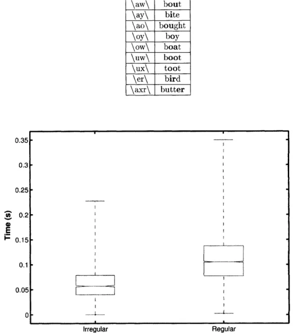
Figure 4-1 shows the distribution of regular and irregular tokens based on their dura-tion using a boxplot (box-and-whiskers plot). The boxplot is a useful way of plotting

Table 4.1: List of vowels used to denote regions of regular phonation along with an example word 0.35 E \iy\ \ey\ \ae\ \aa\ \aw\ \ay\ \ao\ \oy\ \ow\ \uw\ \ux\ \er\ \axr\ beet bait bat bott bout bite bought boy boat boot toot bird butter 0.31 0.25 0.2 0.15 0.11 0.05 0 Irregular Phonation type Regular

Figure 4-1: Duration of regular and irregular tokens L~.

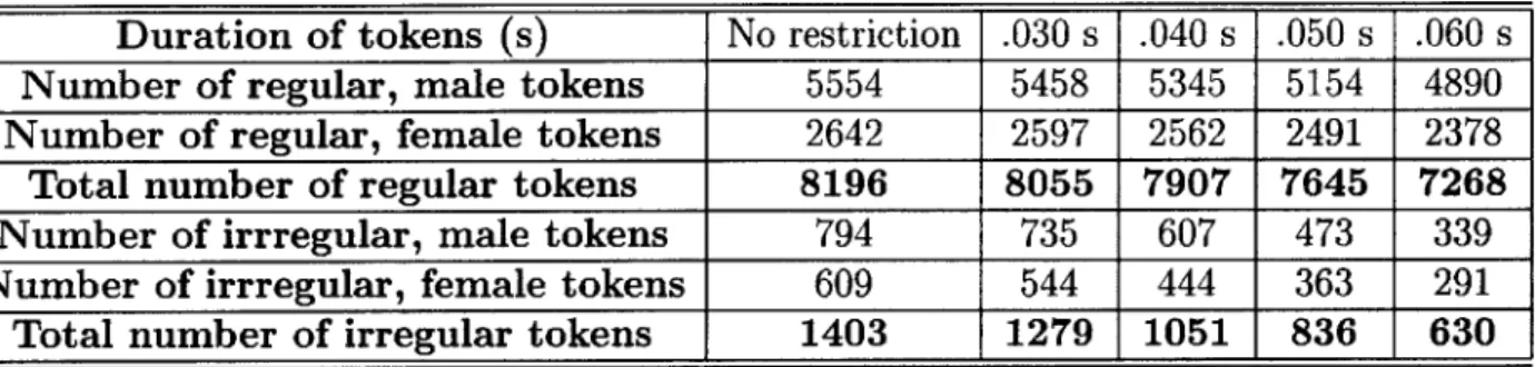
Table 4.2: Number of regular and irregular tokens based on duration of tokens

Duration of tokens (s) No restriction .030 s .040 s .050 s .060 s Number of regular, male tokens 5554 5458 5345 5154 4890 Number of regular, female tokens 2642 2597 2562 2491 2378 Total number of regular tokens 8196 8055 7907 7645 7268 Number of irrregular, male tokens 794 735 607 473 339 Number of irrregular, female tokens 609 544 444 363 291 Total number of irregular tokens 1403 1279 1051 836 630

the five quantiles of the data. The ends of the whiskers show the position of the minimum and maximum of the data whereas the edges and line in the center of the box show the upper and lower quartiles and the median. The whiskers show the be-havior of the extreme outliers. Table 4.2 shows the number of tokens for regular and irregular phonation, broken down by gender, based on the duration of the tokens.

Chapter 5

Method

This thesis uses a knowledge-based approach, rather than solely a data-driven one, to develop a set of acoustic cues that can separate regular phonation from irregular phonation. Different methods were explored to compute and normalize these cues. The separation of these cues was subsequently tested using various statistical clas-sifiers in smaller pilot studies, and a process of iteration resulted in the final choice of four acoustic cues which can distinguish between regular and irregular phonation. This chapter describes these acoustic cues.

5.1

Cue selection

Fundamental frequency, normalized root mean square amplitude, smoothed-energy-difference amplitude and shift-smoothed-energy-difference amplitude are the four cues chosen to distin-guish regular phonation from irregular phonation. Their method of computation and a detailed overview on the rationale behind choosing these cues will be presented in the following section. These cues are chosen based on the observation that irregular phonation is accompanied by clear peculiarities in the signal in the form of either a lack of periodicity, strong variations of the amplitude, very long pitch periods or special forms of the damped wave which are not observed in regular phonation.

Table 5.1: Expected behavior of an ideal FO estimator to distinguish between regular and irregular phonation.

FO output

Irregular (abnormal spacing) < 72 Hz (Blomgren et al., 1998)

Irregular (lack of structure) 0 Hz (i.e. No fundamental frequency estimate)

Regular 86 Hz - 170 Hz (males) (Blomgren et al., 1998) 175 Hz - 266 Hz (females) (Blomgren et al., 1998)

5.1.1

Fundamental Frequency (FO)

This thesis essentially aims to detect two broad categories of irregular phonation -the first type shows distinct irregularities in time or amplitude and is characterized by a lack of structure in the waveform while the other type has abnormal spacing between adjacent glottal pulses relative to the glottal pulse spacing in the local environment. Both these descriptions differ from the quasi-periodic structure of the waveform for regular phonation. This distinction suggests that fundamental frequency could be a valuable cue in separating regular phonation from irregular phonation. Table 5.1 lists the ideal behavior for a FO estimator to classify regular phonation from irregular phonation showing the expected FO ranges for the two types of irregular phonation as well as gender-based, expected FO ranges for regular phonation.

The absence of a robust FO estimator which applies to both regular and irregular phonation is a roadblock in using this cue. Most estimators are specifically designed to compute FO estimates for examples of regular phonation. This thesis uses an FO estimator, based on the filtered-error-signal-autocorrelation sequence to minimize formant interaction, which can provide a reasonable level of separation in the FO es-timates for both regular and irregular phonation (see Table 5.2). A detailed overview of this method is available in Markel & Gray (1976), but the algorithm is briefly

outlined here.

In order to compute the FO estimate, the speech segment is first low-pass filtered using a 12h -order Chebyshev filter with the stop-band ripple 30 dB down and the stopband edge frequency at 1000 Hz. The segment is then pre-emphasized using a 500 Hz single-pole high-pass filter which boosts amplitudes at higher frequencies. This

step counteracts the net decrease in amplitude of -6 dB/octave at higher frequencies (resulting from the sum of a -12 dB/octave decrease in amplitude from the voicing source and a +6 db/octave rise due to the radiation characteristics) during speech production. After processing the resulting segment through a Hamming window of equal length, the autocorrelation sequence for the segment is found. The Levinson-Durbin recursion algorithm is used to find a set of coefficients that model the vocal tract as an all-pole filter using what is commonly referred to as the "autocorrelation method". The coefficients from the Levinson-Durbin algorithm model the vocal tract as a transfer function in the form,

H(z) = an X Zn

where a represents the coefficients from the Levinson-Durbin algorithm.

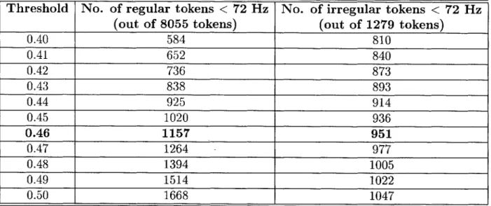
The original segment is filtered using the coefficients from the Levinson-Durbin algorithm to yield the error signal, which is an indicator of the glottal activity at the source. The autocorrelation sequence for the error signal forms the basis for the FO computation. The autocorrelation sequence is first normalized by the peak amplitude at zero lag. Subsequently, all peaks greater than 0.46 over a range from 2.5 ms to half the length of the autocorrelation sequence are selected. The choice of 0.46 as a threshold value is not mentioned in the Markel & Gray algorithm and was selected based on analysis documented in Table 5.2. Specifically, choosing 0.46 as a threshold value results in reasonable FO estimates for a majority of the regular and irregular tokens.

The choice of a particular peak's index provides an estimate for the fundamental period of the segment. The FO estimate is calculated by taking the inverse of the fundamental period. The steps involved in choosing the correct peak index have been itemized below:

- If no peaks > 0.46, then the FO estimate is 0.

- If only one peak is > 0.46, then the associated index is estimated as the funda-mental period.

Table 5.2: Number of F0 estimates below 72 Hz for regular and irregular tokens using different threshold values for the peak-detector in the FO estimator. Ideally, a majority of the irregular tokens, but very few regular tokens, should have F0 values less than 72 Hz.

Threshold No. of regular tokens < 72 Hz No. of irregular tokens < 72 Hz

(out of 8055 tokens) (out of 1279 tokens)

0.40 584 810 0.41 652 840 0.42 736 873 0.43 838 893 0.44 925 914 0.45 1020 936 0.46 1157 951 0.47 1264 977 0.48 1394 1005 0.49 1514 1022 0.50 1668 1047

- If more than one peak is > 0.46, then a test is conducted to determine if all

the peak indices are proportional to each other within a threshold of 0.02. If the peaks indices do meet this criteria, then the second peak index is estimated as the fundamental period. The first peak is ignored since its choice leads to halving of the actual F0 value.

- if all the above-mentioned criteria fail, the maximum peak above the threshold

value is selected and its index determined as the fundamental period.

Figure 5-1 illustrates the F0 computation on a regular and an irregular token respectively.

5.1.2

Normalized Root Mean Square Amplitude

Most of the examples of irregular phonation encountered during labeling match de-scriptions of vocal fry. The number of glottal pulses per unit time for vocal fry is less than the number for regular phonation due to the abnormal spacing of glottal pulses. Other types of irregular phonation show a similar behavior where

irregulari-1000 (a) 5001 0 0.005 0.01 0.015 0.02 0.025 0.03 Time (s) 1

(d)

No peaks above threshold. FO = 0

0.5 .. .. .. .. .. .. .. .. ..-. . .. . .

0 .0.5/

0.005 0.01 0.015 0.02 0.025 0.03 Time (s)

Figure 5-1: (a) Example of a regular token. (b) The autocorrelation function for (a). (c) Example of an irregular token. (d) The autocorrelation function for (c). The horizontal line indicates the threshold value of 0.46 used in the FO computation. (b) has multiple peaks greater than 0.46; the fundamental period is correctly chosen by the second peak greater than 0.46. In contrast, (d) has no peaks greater than 0.46 and the FO estimate equals the default value of 0.

Now -500 1 .0.5 E 0

Z-

_.

(b) A--2nd peak> threshold pitch period

I

ties in the spacing between glottal pulses lead to a lower number of glottal pulses per unit time compared to regular phonation. This observation suggests that the average signal amplitude estimated over a fixed time window should be greater for a regular segment than for an irregular segment. Figure 5-2 illustrates this hypothesis using an example of a regular and an irregular token.

Root mean square (RMS) amplitude is a common tool used in signal processing to estimate the average amplitude of a signal. The result for the RMS amplitude of the token is normalized by the RMS amplitude of the entire speech signal from which the regular or irregular token is extracted to account for inter-speaker variation in signal amplitude. The assumption using this method of normalization is that the speaker uses the same "speaking level" over the course of the utterance. The mathematical formulation to compute this cue is,

( LU s[1]2)O.5

ARMS - 2n=.5

where s[n] is the regular or irregular token, S[n] is the entire speech signal or utterance in the case of the TIMIT database, N is the length of the entire speech signal in samples and L is 30 ms of the regular or irregular token in samples.

5.1.3

Smoothed-energy-difference amplitude

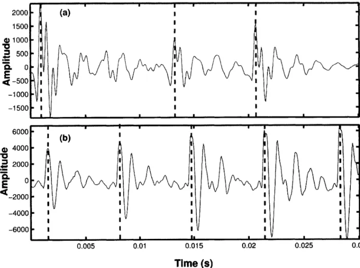
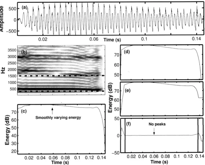
Most examples of irregular phonation in the data-set either match descriptions of vocal fry with widely spaced glottal pulses or show abruptness in the time-domain waveform. This abruptness can be manifested in the form of an "impulse-like" tri-angular pulse, a sudden change in amplitude of a glottal pulse or the appearance of an additional glottal pulse within the normal glottal cycle. It is hypothesized that all these behaviors should be characterized by a rapid transition of energy within the irregular segment. Regular phonation, on the other hand, will not generally show such rapid variations in energy. In order to test this hypothesis quantitatively, the smoothed-energy-difference amplitude cue was formulated.

2000-

_(a)

E

E

Time (s)

Figure 5-2: (a) Example of an irregular token. (b) Example of a regular token. Both are taken from the same speaker and are of the same duration to avoid inter-speaker variablity in signal amplitude. The dashed vertical lines indicate the glottal pulses in the token. (b) has five glottal pulses, compared to three for (a) and hence a higher average signal amplitude.

Hamming window size of 16 ms was chosen to window the token while calculating the FFT in the form,

512

X [k] = 1 x[n]w[n]e-jw,"

n=1

where x[n] is the input segment, w[n] is the 16 ms Hamming window and X[k] is the FFT of x[n].

Since the FFT is symmetric in frequency, only the first 256 points of the FFT are analyzed. The window is shifted by 1 ms and the FFT is calculated recursively across all the segments in the token. These values are squared eventually giving a matrix of size (256 x nFrames), where nFrames is the number of frames in the token where the FFT has been computed. This matrix contains the energy information for the token across all frequencies. The energy in each frame is averaged between 300 Hz - 1500 Hz and the 10 * logio of the values are used to compute a matrix of size

(1 x nFrames) giving one averaged energy value per frame for the token.

The choice of lower frequencies is valid since most of the energy in vowels, which are used as examples of regular phonation, is concentrated in this range of frequencies with the first formant rarely dipping below 300 Hz. The upper limit of 1500 Hz was chosen since it resulted in the best separation in the smoothed-energy-difference values for regular and irregular tokens as documented in Table 5.3.

The energy values found previously were averaged in time using different smooth-ing window sizes - the initial choices being 10 ms and 16 ms respectively. The choice of (10 ms, 16 ms) was based on the rationale that both these window sizes would in-clude at least one glottal pulse in the time-domain waveform for regular phonation resulting in a small difference between the two smoothed-energy waveforms. How-ever, in many cases of irregular phonation with widely-spaced glottal pulses, a 10 ms window size would not encompass one glottal pulse resulting in a larger difference in energy between the pair of smoothed-energy waveforms.

The difference between the smoothed averaged energy values using the two win-dow sizes, called the smoothed-energy-difference waveform, helps separate abrupt variations in energy from smoothly-varying variations in energy. Since the energy in